Controlled Impedance-Admittance-Torque Nonlinear Modeling and Analysis of Modern Power Systems

Abstract

Modern power systems are continuously transformed into decentralized ones where distributed generation (DG) plays a key role. Almost all the different distributed energy resources (DERs) are connected in geographically dispersed places through controlled power electronic interfaces in a manner that essentially affects the dynamic performance and control of the whole power system. Simultaneously, rotating machines in power production or absorption, dominate the system response and stability. In this new frame, this paper proposes a novel generalized dynamic representation and full scale modeling of a modern power system based on the well-known impedance-admittance (IA) network model for the electricity grid, substantially extended to include in detail both the power converter devices by considering the controlled power electronic dynamics and the electrical machines by inserting their full electromechanical dynamics. This formulation results in a holistic nonlinear dynamic description, defined here as controlled impedance-admittance-torque (CIAT) model of the whole system which features common structural characteristics. The model is deployed in state space, involves all the controlled inputs in DG, namely the duty-ratio signals of each power converter interface, all the other external inputs affecting the system, namely all the known or unknown voltage, current, and torque inputs. As shown in the paper, the proposed CIAT model retains its fundamental properties for any DG and network topology, standard or varying. This enables the compression of the accurate analytic power system dynamic description into a matrix-based generic nonlinear model that can be easily used for analysis studies of such large-scale systems. Taking into account the nonlinear nature of the CIAT matrix-based model and the persistent action of the external inputs, Lyapunov methods deployed on recently established input to state stability (ISS) notions are systematically applied for the system analysis. Hence, the traditionally used small-signal model-based analysis that suffers from the intermittent and continuously changing operation of DERs is completely substituted by the proposed formulation. A modern power system example with different DERs involved is analyzed by this way and is extensively simulated to verify the validity of the proposed method.

1. Introduction

Modern power systems are being effectively reshaped both in structural and operating manner as dictated by environmental concerns and newly imposed efficiency and reliability regulations. The current global trend for including geographically dispersed renewable energy sources (RES) undoubtedly leads to new layouts mostly at the distribution level, where active loads locally coexist with conventional passive ones, with the transmission grid being affected as well. Nowadays, the well-known vertical and centralized power system structure is continuously transformed to a decentralized one that needs efficient cooperation between the actual physical system and the local and upper control and management layers set for regulating and monitoring the whole power grid.

In this frame, distributed generation, mainly based on the high penetration of distributed energy resources (DERs) such as different RES, storage units, etc., and new local grid structures, such as microgrids, play a key role in the electricity grid deployment [1]. However, the intermittent behavior and the stochastic nature of power generation of some DERs or the maximum power point (MPP) operation of others, have a clear impact not only on the grids’ operation planning, but on the overall system stability as well, especially in cases of large-scale DER integration. In contrast to centralized power systems where generation is solely based on large synchronous machines (SM) operating at their nominal synchronous speed and contributing to the overall system stability through their large rotor inertia, modern distributed generation (DG)-based power environments are characterized by lower inertia. A high number of different DERs coexist with SMs, with many of them not necessarily providing beneficial inertia characteristics to the grid, i.e., photovoltaic (PV) stations. Furthermore, since each DER is usually connected locally via inertialess power electronic interfaces at the grid side, abnormal situations and instability phenomena are even more common [2]. Nevertheless, these undesired effects can be addressed by implementing appropriate local control schemes and applying, at any time instant, suitable input commands, offering active and reactive power regulation and contributing to voltage and frequency stability through decentralized provision of ancillary services [3].

Certainly, along with the unique possibilities introduced in this situation, the complexity of power grids is also significantly increased. This leads to entirely new and different needs and requirements in order to conduct analysis studies for these kinds of systems compared to the traditional methods applied for conventionally structured grids. In this sense, the accurate modeling of the system is of the utmost importance not only for operation handling and performance evaluation reasons but to establish and verify stability under variable and intermittent operating conditions. Several approaches have been proposed in the literature in order to reach a universal and generalized modeling framework, capable of accurately representing the new grid formulation [4]. Among these newly introduced methods, the graph theory fundamentals combined with the complex network notion have been widely utilized as a means to establish an effective analysis tool [5]. However, most of the proposed designs are developed by contrasting other cross-disciplinary network theory basic approaches made for computer, communication, or other systems [6,7,8]. This presents an obvious disadvantage since the application of these schemes does not take into account the increased complexity met in new power grid network formulations, as introduced by control and management actions, while these implementations also neglect basic dynamic characteristics for the sake of model simplification. Some network formulation approaches feature strictly topological based models [9], which of course do not include electrical characteristics of the grid, while other component-based models employ arbitrary probabilistic models in order to assess the vulnerability of the grid due to component failure possibility [10]. Regarding the dynamic models proposed, some of them consider the dynamic behavior of active devices such as power converters [11], while others include simplified machine models of only one type in the dynamic formulation [12]. A last endeavor to formulate modern power systems by their Hamiltonian representation is not completed to involve all the parts and topologies [13]. Indeed, it is noted that according to the authors knowledge, none of the proposed modeling procedures result in a generic linear or nonlinear dynamic description of modern grids. Furthermore, the main purpose in the majority of these cases aims to examine the power grid from a reliability or from a vulnerability analysis point of view and do not focus on establishing either local or global stability conditions.

In terms of applying the second stage beyond modeling, which is to analyze system stability, the validity of such a study relies on both the accurate dynamic representation of the examined system as well as the appropriate stability tool to be used. In fact, these two aspects are intertwined since the system model itself can provide insight about the implementation of the most suitable stability analysis technique, while some models can be modified so as for a particular method to be applied. Taking this into account, one of the most popular method used in relevant stability studies is based on the small-signal analysis [14], which allows application of well-known linear system theory techniques. This obviously presents the advantage of easy and straightforward implementation, capable of examining the power system performance and stability but only close to a certain predefined operating point, while the results of the analysis are in many cases largely dependent on the system parameters. This is inefficient in modern power system analysis where the power injected and absorbed is mostly unpredictably changing in a continuously varying grid and DER topology.

On the other hand, several nonlinear techniques such as Lyapunov-based ones have been considered [15], since they match with the nonlinear structure of modern power systems. These methods utilize the actual structure of the model by considering inherent properties in it, i.e., the handled energy, through the construction of suitable Lyapunov-type functions and thus overcome drawbacks related to operating point and system parameter dependency. In fact, this approach exhibits quite satisfactory results when the system states converge to zero equilibria [16]. However, this is rarely the case with power system operation and even less so when a modern power grid is considered. There are varying and intermittent external controlled or uncontrolled inputs persistently acting on the system to drive its states to nonzero equilibria in a lot of different values as the external inputs tend each time to different steady state conditions. To examine the stability around nonzero equilibria, the standard Lyapunov-based technique is then deployed not on the natural model but on the corresponding incremental dynamic model obtained around the particular equilibrium [17]. By this method while the problem is transformed to the study of the equivalent zero equilibrium of the incremental model, it becomes very hard or even impossible to determine suitable Lyapunov functions in cases of large-scale nonlinear systems, such as power systems. Thus, on one hand, the simplified small-signal representation does not hold true anymore due to complexity and varying conditions of a modern power system; on the other hand, the required dynamic nonlinear modeling of modern dispersed power systems can be efficiently formulated for specific cases only [18], with complex characteristics that according to the traditional nonlinear techniques are difficult to analyze [19]. Moreover, it is clear that the latter representation stands very far from being established as a general tool for studying the dynamic response and stability of power systems.

Our aim is to develop a systematic and global solution to confront the difficult task of analyzing such complex systems by suitably combining an accurate model formulation possessing common properties with an advanced nonlinear analysis method. The focus is to adopt a method compatible with the actual nonlinear model and capable of examining nonzero equilibria as it is the case with real-world power systems. In particular, the first key point of this task is to develop a generalized dynamic description and modeling of modern power systems which can effectively include any possible grid and DG topology and different static or rotating installations operating in a wide and varying range. The second issue is to establish a novel analysis tool that can exploit the fundamental system characteristics in order to evaluate in a common and immediate way the dynamic response of the system, namely the stability and convergence at the recommended nonzero equilibria. In this frame, this paper proposes a generalized network-based representation of the power grid, deployed on the grid impedance-admittance (IA) accurate model [20]. This formulation is initially modified into the controlled IA (CIA) model since it is extended to include the controlled power converter interface dynamics by considering their nonlinear mean-value models. In the sequel, the corresponding nonlinear electromechanical torque dynamics of several electric machines used in different conventional power plants or wind turbine stations or large rotating loads are considered. This formulation results in the complete nonlinear model of the system, defined as controlled impedance-admittance-torque (CIAT) model which absolutely covers the need of the accurate representation of a modern power system.

Nevertheless, the most important contribution resulted by the proposed formulation is twofold: firstly, CIAT constitutes a generic nonlinear representation in state-space which can be abstractly reduced in suitable matrix description with the state vector to involve three distinguished sub-vectors, the one representing the grid current vector, the second representing the grid buses voltage vector, and the third representing the different machines rotor angular speed vector. The model is formulated to include directly all the controlled inputs, namely the duty-ratio components, of the different power converter interfaces and any other controlled voltage, current, or torque input. All the other constant or varying, voltage or current source inputs in the electric part or torque inputs in the mechanical part are considered as unknown and bounded external disturbance inputs. Secondly, the aforementioned CIAT formulation of the accurate nonlinear model, retains the same structure independently from the system changes in topology or operating conditions. A fact that features common characteristics in the entire system which are exploited in a common and systematic manner to create a specific tool for power system analysis. Therefore, as caused by the whole system nonlinear representation, the proposed analysis is based on the results of the contemporary study presented in [21], which provides a complete, new theoretical framework to study such nonlinear systems by combining Lyapunov-based methods with the input-to-state stability (ISS) notion. Hence, the rigorous stability analysis conducted on this basis, eventually indicates that a sufficient condition for proving either global or local stability and, under realistic input boundedness conditions, state convergence to the expected nonzero equilibrium is simply established and always guaranteed when the system is described by a CIAT model. The proof is given in detail in the paper, making clear that constructing the system CIAT model is simultaneously adequate to conclude stability. Thus, the CIAT modeling stands automatically as power system analysis tool as well. Therefore, the advantages of the proposed modeling and analysis procedure can be identified in multiple levels: (i) the power system dynamics are extensively examined by considering all contributing subsystems and apparatus, i.e., the grid network, the power electronic interfaces, and the electromechanical components, (ii) the generalized CIAT formulation itself can be obtained for any such a power system topology, standard or varying, and retains its fundamental properties in any case, (iii) the stability analysis at the physical level is guaranteed as far as the CIAT model is valid for the particular system, (iv) the integration of upper networked layers of optimization and management into the system, becomes very simple since the executed schemes may act on the different controlled inputs of the physical aspects under the discussed stability conditions.

The remainder of the paper is organized with the following structure. In Section 2, the actual complete power network description is provided in sequential stages; the basic properties of the IA model representation are given in a form that takes into account typical passive element-based network topologies. It is also shown, that these properties are retained when the dynamic behavior of controlled power electronic components is taken into consideration which, however, changes the conventional IA model into a controlled IA (CIA) structure. This description is finally integrated to include also the dynamics of the electric machines connected to the system in order to complete the proposed CIAT generalized formulation of the system. The main stability results are derived in Section 3. Specifically, the needed ISS-based background for the proposed analysis is presented and then an extensively detailed procedure is performed, covering all possible grid-forming situations. A rigorous proof is deployed in order to establish the system stability and convergence of the state trajectories to equilibrium. In Section 4, the proposed approach is evaluated by considering a representative example case-scenario involving a typical modern DG-based power system so as to demonstrate the validity of the CIAT modeling and to verify the analysis both theoretically and through simulated results. Finally, the main contributions are summarized in the form of conclusions in Section 5.

2. Power Grid Network Formulation

A power grid is naturally an electric network consisting of nodes (buses) and links (lines). All substations, generation sources, loads, etc. are directly connected or via a power electronic converter to buses, while transmission or distribution lines are used to connect the buses to each other. This fundamental view of the grid constitutes the basic framework for constructing a network representation of such a system, at least at the physical level. It is among the basic aims of this paper to build upon this consideration in order to derive a systematic way of modeling a power grid in a manner which serves the accurate performance evaluation and enables the application of advanced nonlinear stability analysis techniques so as to verify the stable behavior of the system.

2.1. Impedance-Admittance (IA) Modeling of a Power Grid

A set of two methods has been extensively used in order to systematically derive the dynamic equations describing a network, namely the combination of the node and the loop method [22]. By applying this set to the modern power system paradigm, the node method considers the voltage of a bus as a system variable, whereas in the loop method the current flowing through a link is treated as a variable. Following this approach, the complete mathematical representation of a power grid can be derived and is referred to as the impedance-admittance (IA) representation where admittance description is the result of the node method application and correspondingly, impedance description relates to the implementation of loop method.

According to the IA modeling formulation, for any ac or dc circuit model featuring lumped parameter elements in its structure, the following holds true:

1.

The link impedance representation is

$$\left[pZ+p^{-1}C+R\right]i_{ac}+E{v}_{ac}=V_{ac}$$

(1)

where p and p⁻¹ are the derivative and integral operators respectively, $i_{ac}$ represents the vector of all link currents, $v_{ac}$ is the vector containing all node voltages, $V_{ac}$ stands for all the external voltage inputs of the system, and $E$ is a matrix of appropriate dimensions. Additionally, the component-parameter impact on the link-system is introduced in this formulation via matrices Z, C, and R, which express the inductance, capacitance, and resistance, respectively.

In a corresponding manner:

2.

The node or bus admittance representation can be obtained as

$$\left[p\tilde{C}+p^{-1}\tilde{Z}+\tilde{B}\right]v_{ac}+\tilde{E}{i}_{ac}=I_{ac}$$

(2)

where matrices $\tilde{C},\hspace{1em}\tilde{Z},\hspace{1em}\tilde{B}$ represent the capacitance, inductance, and conductance, respectively, and $\tilde{E}$ is a matrix of appropriate dimensions and vector $I_{ac}$ contains all the external current source inputs.

The IA model in its general form as given by Equations (1) and (2) can be used to describe any node and link in any possible circuit topology. However, is worth noting that in practice, either classical or modern power grids tend to not have inductive components connected to their buses as they also do not have capacitive elements along their lines. Therefore, the previous model can be effectively simplified as

$$\left[pZ+R\right]i_{ac}+E{v}_{ac}=V_{ac}$$

(3)

$$\left[p\tilde{C}+\tilde{B}\right]v_{ac}+\tilde{E}{i}_{ac}=I_{ac}$$

(4)

where now only the inductance and resistance are considered in the impedance model of Equation (3), while the capacitance and resistance (in the form of conductance) are exclusively taken into account in the admittance representation of Equation (4).

Remark 1.

Normally, in power system networks it is a standard way to use Equations (3) and (4) for the system description, e.g., it is correct to simplify Equation (1) into Equation (3) without losing generality since when capacitance in power lines appear this can be separately handled by an admittance equation. However, there are rare cases where this does not hold, especially in different load equivalent circuits. Therefore, for the completeness of the proposed formulation it is proven in theAppendix Athat also the full case representation as in Equations (1) and (2) can be eventually transformed into a form similar to Equations (3) and (4).

Considering a typical symmetric and balanced three-phase ac power system, the application of Equations (3) and (4) on each phase provides a system of three ac dynamic equations with only the two of them being independent. It should be noted that this assumption is typical for transmission systems, whereas it can be applied to distribution networks of medium/low voltage as well, in which additional assumptions regarding load balancing have to be considered. Nevertheless, since the three-phase ac system contains all variables in sinusoidal form, all these are rarely convenient for analysis purposes. Hence, the system is usually represented by phasors [23] for conventional power systems analysis, usually in steady state, or it is transformed into a two-axis system by adopting the d-q reference frame through Park’s transformation [24], usually for dynamic performance studies. The latter representation displays clear advantages, especially when the synchronously rotating d-q reference frame is adopted since all quantities become time-invariant with all sinusoidal variables to be constant in steady-state [24]. This approach reduces significantly the dynamic model complexity; a fact much desired in large networks and particularly useful in control design and dynamic analysis for both classical and modern power systems.

Thus, in this work, the synchronously rotating d-q reference frame is applied in the IA description, but the applied transformation does not come without a cost. The basic model structure as given by Equations (3) and (4) is retained, but a newly introduced coupling between the d- and q-axis components of system variables, namely the currents and voltages, has to be considered. In particular, for the impedance description, the damping matrix R is now replaced in the d-q frame, by $D-J$, where $J$ is a suitable skew-symmetric matrix representing the coupling between the d- and q-axis current components. In a similar manner, the damping matrix $\tilde{B}$ in the admittance model of Equation (4) is replaced in the d-q frame, by a new $\tilde{D}-\tilde{J}$ matrix in order to account for the coupling between the d- and q-axis voltage components, as represented by the skew-symmetric matrix $\tilde{J}$. Additionally, considering the inherent structure of the network, the vector ${\left[E{v}_{ac}\hspace{1em}\tilde{E}{i}_{ac}\right]}^T$ of system (Equations (3) and (4)) can be transformed in the d-q frame as

$$\left[\begin{array}{c}Fv\\ \tilde{F}i\end{array}\right]\equiv \left[\begin{array}{cc}0& F\\ \tilde{F}& 0\end{array}\right]\left[\begin{array}{c}i\\ v\end{array}\right]$$

(5)

where $i,\hspace{1em}v$ stand in the d-q frame for $i_{ac},\hspace{1em}{v}_{ac}$, respectively; $I,\hspace{1em}V$ stand in the d-q frame for $I_{ac},\hspace{1em}{V}_{ac}$, respectively, and matrix $\left[\begin{array}{cc}0& F\\ \tilde{F}& 0\end{array}\right]$ is always a skew-symmetric one, i.e., $\tilde{F}=-F^T$.

Hence, the resulting IA system description is given in the synchronously rotating d-q reference frame as

$$\left[\begin{array}{cc}M& 0\\ 0& \tilde{M}\end{array}\right]\left[\begin{array}{c}pi\\ pv\end{array}\right]=-\left[\begin{array}{cc}D-J& F\\ -F^T& \tilde{D}-\tilde{J}\end{array}\right]\left[\begin{array}{c}i\\ v\end{array}\right]+\left[\begin{array}{c}V\\ I\end{array}\right]$$

(6)

where matrices Z and $\tilde{C}$ are replaced in the d-q synchronously rotating frame by $M$ and $\tilde{M}$.

It is also noted that the proposed IA model has the following remarkable property.

Property 1.

The proposed IA formulation given by Equation (6) has the following features:

1. 

matrices $M$ and $\tilde{M}$ are constant, symmetric, and positive definite,

2. 

damping matrices $D$ and $\tilde{D}$ are constant, symmetric, and at least positive semi-definite,

3. 

the skew-symmetric matrices $J$ and $\tilde{J}$ are linearly dependent from the synchronous angular frequency, ${\omega }_s$, of the rotating system reference frame,

4. 

all external uncontrolled inputs of the system are either voltage or current sources and are included in the vector ${\left[\begin{array}{cc}V& I\end{array}\right]}^T$.

In formulation of Equation (6), matrix F is of rather high significance, as its elements depend from the nature of the modelled grid. In conventional power system networks, all elements of F are referred to passive components and, therefore, are constant. On the other hand, if active or controlled devices, such as power converters, also exist in the system topology, then some of the elements in F are directly dependent from the input signals of these interfaces. Nevertheless, it is important to note that by including such devices in the formulation, the standard structure of the model remains consistent in any case. By exploiting this fact, it is possible to incorporate any controlled component in this formulation as explained in the next subsection.

2.2. Controlled Impedance-Admittance (CIA) Modeling of Power Grids with Active Grid Components

Since many types of converter-based installations have been recently introduced in power systems, it is important to note that all major ac/dc interface configurations, such as voltage source converters (VSCs) [25], or current source converters (CSCs) can be described by employing the IA formulation. The input and output of such a converter device, including any combination of passive circuit components connected to it, can be considered as a node, in accordance with the admittance model. Additionally, the lines connecting the converter to the grid almost always feature an inductor-based filter, so the impedance model can be applied for them as well [11]. It is apparent that the dynamics of the converter switching elements need to be incorporated in the original IA description. The dynamic equations of power converters naturally contain discontinuous functions to describe the on-off switching operation of the power electronic elements which, however, clearly complicate the system model and analysis. Nevertheless, the adoption of the average model can effectively substitute the original switching converter model by employing continuous functions for the converter duty-ratio signals to describe the on-off operation of converters switched by the pulse width modulation (PWM) technique. As it has been proven in [17,26], the average models of the power electronic interfaces are more accurate, the larger the PWM frequency becomes, whereas it renders the converter modeling compatible with the rest grid representation. Thus, considering the average model of such a dc/ac converter in the synchronously rotating d-q reference frame, then the duty-ratio d- and q-signal components are suitably inserted in separate terms into matrix F.

In a similar manner, dc/dc power converters of all types, used in a variety of power subsystems connected to the grid, i.e., to interface photovoltaic installations or energy storage stations, can be also represented by the IA model even more conveniently since no reference frame transformation is needed to be applied, while they are directly compatible with the synchronously rotating d-q reference frame IA representation.

In all cases, the dynamics of the different power converter interfaces are incorporated in the original description of Equation (6) wherein now the matrix F becomes a function of the duty-ratio signals. Keeping in mind that power converters are strictly regulated devices, they can feature appropriately designed control schemes [27] in order to ensure a desired operation in a stable and efficient manner. Hence the actual controlled input of a power grid involving power electronic devices is given by the vector

$$m={[m_1\hspace{0.17em}{m}_2\hspace{0.17em}\dots \hspace{0.17em}{m}_k\hspace{0.17em}\dots \hspace{0.17em}]}^T$$

(7)

where $m_k$ represents the k th duty-ratio controlled input of the system.

Therefore, the controlled impedance-admittance (CIA) model is obtained as follows:

$$\left[\begin{array}{cc}M& 0\\ 0& \tilde{M}\end{array}\right]\left[\begin{array}{c}pi\\ pv\end{array}\right]=-\left[\begin{array}{cc}D-J& F(m)\\ -F^T(m)& \tilde{D}-\tilde{J}\end{array}\right]\left[\begin{array}{c}i\\ v\end{array}\right]+\left[\begin{array}{c}V\\ I\end{array}\right]$$

(8)

One can see that the CIA model is now nonlinear since the controlled input vector $m$ is included in F. It is pointed out that now Equation (8) also includes all the IA modelled components in the synchronously rotating d-q reference frame, i.e., Equation (8) represents a generalization of Equation (6) with the controlled power converter models involved.

It is noted that in practice, most of control design implementations feature saturation mechanisms in the modulation of vector $m$ as to ensure operation in the linear region [28]. Therefore, the controlled input signals provided to power system converters are clearly considered to be bounded and are quite reasonably assumed to tend in piecewise constant values after any transient caused by the uncontrolled input vector (of the external voltages and currents) changes; a fact that is particularly useful for different equilibria to exist and allows us to consider permitted constant values for the duty-ratio inputs in studies of their stability when system states reach the corresponding steady state.

2.3. Complete Generalized Controlled Impedance-Admittance-Torque (CIAT) Modeling with the Rotating Electromechanical Dynamics Included

As discussed in the previous subsection, the inclusion of controlled power electronic interfaces in a grid structure results in the careful and detailed representation of the accurate, very fast converter dynamics. This directly requires giving an equal effort for the dynamic representation of the electric machines as well, in order to reach a power system formulation compatible with the one describing the fast dynamics of power converters. Nowadays, many types of electric machines in different configurations can be situated in a modern decentralized power system, with almost all of them featuring nonlinear dynamic models. It is noted that electric machines are intrinsically complex electromechanical systems, involving both an electric part and a rotating mechanical part interacting with each other. The modeling of the electric part of voltage forced machines, is directly compatible with the IA or CIA representation by adding the electromotive force term $V_{ef}$ in the impedance equation. Then the impedance equation in Equation (8), is modified to

$$M[pi]=-[D-J]i-F(m)v+V-V_{ef}$$

(9)

On the other hand, the action of rotating masses creates inertia-related effects with their angular speed dynamics to take place on a much larger time scale than the one observed in transmission lines or active devices which is therefore inserted by a separate dynamic equation. Hence the mechanical dynamics of electric machines are described by their torque equations, comprising both the external torque applied on the rotor and the electrical one induced by the electromagnetic interaction between the stator and the rotor, as follows

$$H{\dot{\omega }}_r=-\overline{D}{\omega }_r-T_m+T_e$$

(10)

where ${\omega }_r$ is the rotor angular speed vector containing all the particular machine angular speeds, $H$ is the diagonal matrix with all the particular rotor inertias, while $\overline{D}=diag\left\{b_1\hspace{0.17em}{b}_2\hspace{0.17em}\dots \hspace{0.17em}{b}_k\hspace{0.17em}\dots \hspace{0.17em}\right\}$ denotes the rotor damping matrix with all the particular damping coefficients $b_k$ involved. Additionally, $T_m$ represents the applied external mechanical torque vector and $T_e$ expresses the corresponding electric torque vector. The torque signs are so selected to comply with motor operation. It is to be noted, that the last term in Equation (10) can be always expressed in the form of combined currents originating from the windings located on either or both the stator and rotor parts of the machine, hence, generally the torque variables are directly related to the current vector in a nonlinear fashion as follows [24],

$$T_e=G^T(i)i$$

(11)

It is also noted that in cases where permanent magnets substitute the electric machine excitation circuits, then matrix G becomes constant.

The internal energy balance between the rotating part and the electrical one of a machine, causes the electromotive force term of Equation (9) to take the form

$$V_{ef}=G(i){\omega }_r$$

(12)

i.e., the electromotive force is as usual a nonlinear function depending on ${\omega }_r$.

Considering the torque Equation (10) in the CIA model and taking into account the modified impedance Equation (9) with $T_e$ and $V_{ef}$ given by Equations (11) and (12), the complete controlled impedance-admittance-torque (CIAT) model is obtained

$$\left[\begin{array}{ccc}M& 0& 0\\ 0& \tilde{M}& 0\\ 0& 0& H\end{array}\right]\left[\begin{array}{c}pi\\ pv\\ p{\omega }_r\end{array}\right]=-\left[\begin{array}{ccc}D-J& F(m)& G(i)\\ -F^T(m)& \tilde{D}-\tilde{J}& 0\\ -G^T(i)& 0& \overline{D}\end{array}\right]\left[\begin{array}{c}i\\ v\\ {\omega }_r\end{array}\right]+\left[\begin{array}{c}V\\ I\\ -T_m\end{array}\right]$$

(13)

According to this representation, all dynamics deriving from electromechanical components situated in the grid can be effectively included in a concise manner, compatible with the already established power network description. Since the CIAT model can be used to represent fundamental modern power system structures, it is crucial to further demonstrate all features imposed by this modeling. To this end, in the following Property 2, the original features given by Property 1 are expanded to the general case.

Property 2.

In CIAT generic modeling given by Equation (13), the following hold true:

1. 

the matrix at the left side of Equation (13) is always constructed as a block diagonal matrix with all involved matrices $M$, $\tilde{M}$, and $H$ are constant, symmetric positive definite,

2. 

the first matrix at the right side of Equation (13) can be always written as a sum of a constant negative definite (or negative semi-definite) damping matrix $D_s$, and a generally non-constant skew-symmetric matrix $J_s$,

$$D_s=blockdiag\left\{\begin{array}{ccc}-D,& -\tilde{D},& -\overline{D}\end{array}\right\}\mathit{,}\mathit{and}\mathit{,}{J}_s=\left[\begin{array}{ccc}J& -F(m)& -G(i)\\ F^T(m)& \tilde{J}& 0\\ G^T(i)& 0& 0\end{array}\right]$$

(14)

3. 

the last vector ${\left[\begin{array}{ccc}V& I& -T_m\end{array}\right]}^T$ at the right side of Equation (13) is now extended to include all the external mechanical torque inputs $T_m$ that act on the rotating machine masses. It is also noted that in the generalized model, vectors $V$ and I may contain controlled components; in this case the vector is split into two distinct vectors, the first to include the controlled parts of $V$ and I and the second to include all the external uncontrolled inputs that are considered all bounded (known or unknown tending to constants in steady state).

Certainly, as the generalized CIAT description (Equation (13)) engulfs all possible grid-forming layouts and can accurately represent power grids where conventional lumped elements coexist with active devices and electromechanical components the properties previously discussed are very essential. This is due to the fact that the addition or subtraction of a grid or power component does not modify the model properties and the general structure itself but only affects both the system dimension and the internal form of the different sub-matrices.

Beyond the systematic modeling procedure proposed, it is among the basic aims of this work, in a second stage, to appropriately exploit the general features and properties of the CIAT model to facilitate the establishment of strong stability results for power systems by suitably applying advanced nonlinear procedures of analysis, specified to be compatible with the standing nonlinear model structure. To that end, the main task deployed in the next section is devoted to extract in a straightforward and generic manner, the sufficient conditions for ensuring stability of such a complex dispersed power system and the corresponding constraints for extending the proof to convergence properties of all the system trajectories to equilibrium.

3. Analysis of System Stability and State Convergence to Equilibrium

Studying and verifying stability of power systems is typically a cumbersome process, mainly due to the nonlinear nature of the models describing them and the large variety of inputs acting on different apparatus to regulate the injected or absorbed power. Hence in conventional centralized power systems there exist many different methods to confront the stability problems mainly distinguished by the short or long-term response of an equivalent to a synchronous generator-based control area of a power system [29]. Small signal analysis is usually applied on simplified linear systems models, whereas nonlinear techniques are rarely accomplished. The adversities of such analysis are greatly intensified when widely dispersed DG-based power systems are considered, since many other factors have to be taken into account. The bidirectional flow of power in modern power systems, the fast control capabilities of the power electronic interfaces installed in DERs and the widely variable range of operation imposed by the intermittent and unpredictable production of many RES, require a novel, more accurate, and holistic studying tool. Keeping in mind the accurate and entirely compressed nature of the CIAT model, our intension is to appropriately use this model in order to establish the sufficient conditions for ensuring stability of modern power systems. This is not an easy task due to the nonlinearities involved in the model, the large number of controlled and uncontrolled inputs of the system which lead to a variety of nonzero equilibria. To achieve this target, it is necessary to deploy a specific advanced nonlinear analysis dedicated to providing generic results for these kinds of system models.

In nonlinear system analysis when nonzero equilibria are considered for systems with controlled or uncontrolled inputs that tend to constant values in steady state, such as the ones previously discussed in the CIAT model deployment, it is by definition convenient to see their analysis in view of the input to state stability (ISS) notion. Fortunately, as shown very recently in [21], ISS has been decisively expanded from the simple stability notion of bounded input bounded state (BIBS) property into verifying system state convergence to nonzero equilibria. It has been already proposed as an effective Lyapunov-based tool in studies of simple traditional power systems and as is proven in [21], it seems to provide strong global or local stability and convergence properties for the examined system under some mild conditions. In this paper, it is further proven that the proposed generic system CIAT model can satisfy all the required conditions for applying this method in a systematic and common way. A key point in the scope of the present analysis is to specify the required conditions for ensuring stability around nonzero equilibria as it is the case for real-world modern power systems. To this end, based on the ISS notion, an extended theoretical framework is employed to serve the twofold aim of extracting the sufficient conditions to ensure stability and sequentially, of proving system-state convergence to an equilibrium, globally or locally inside a defined region of attraction. The proposed analysis approach is shown to be valid for a variety of cases considered by different grid configurations featured in the generalized system formulation described by Equation (13).

As CIAT model belongs to the general form of controlled nonlinear systems that are externally enforced by permanent bounded inputs, in the next subsection, some important preliminary results related to the ISS concept are presented, which are utilized to derive the main results of this study.

3.1. Basic Notations, Preliminaries, and Recent Results for ISS Systems

The notations and terminology used for the presentation of these fundamental results are taken as in [30,31] and are adopted throughout the rest of the analysis. For the readers’ convenience the most basic amongst them are the following: the field of real numbers is denoted by $ℝ$, with ${ℝ}^n$ and ${ℝ}^m$ expressing the real coordinate spaces of n and m dimensions, respectively. In these spaces, $\Vert \cdot \Vert$ is used to denote the Euclidean norm. Additionally, all the presented results concern nonlinear externally enforced systems of the form:

$$\dot{x}(t)=f(x(t),\hspace{0.17em}u(t))$$

(15)

where state $x(t)\in S$, input $u(t)\in S_u$, and $f:S\times S_u\to {ℝ}^n$ is piecewise continuous in t and at least locally Lipschitz in x and u, with the sets S and $S_u$ being defined as:

$$S=\{x\in {ℝ}^n:\Vert x\Vert \le r\},\hspace{1em}{S}_u=\{u\in {ℝ}^m:{\sup }_{t\ge 0}\Vert u\Vert ={\Vert u\Vert }_{L\infty }\le r_u\}$$

Additionally, the unforced version of system (Equation (15)), i.e., $u=0$, is considered as

$$\dot{x}(t)=f(x(t),\hspace{0.17em}0)$$

(16)

This kind of nonlinear system can be characterized as l-ISS or purely ISS according to the following Definition.

Definition 1.

[32].The system of Equation (15) is defined to be locally input-to-state-stable (l-ISS) if there exists a class $𝒦$ $ℒ$ function β and a class $𝒦$ function γ and positive constants $k_1$ and $k_2$ such that

$$\Vert x(t)\Vert \le \beta (\Vert x(0)\Vert ,t)+\gamma ({\sup }_{0\le \tau \le t}\Vert u(\tau )\Vert )$$

(17)

for all $t\ge 0$ and $x\in S$, $u\in S_u$ with $\Vert x(0)\Vert <k_1$ and (ess) ${\sup }_{t\ge 0}\Vert u\Vert ={\Vert u\Vert }_{L\infty }<k_2$. The system is said to be input-to-state stable (ISS) If $S={ℝ}^n$, $S_u={ℝ}^m$ and Equation (12) holds true for any initial state $x(0)$ and any bounded input $u(t)$.

Definition 1 provides the necessary properties that a system of the form of Equation (15) needs to possess in order to be characterized as either l-ISS or ISS. Intrinsically, both ISS properties are verified by establishing a suitable Lyapunov-type function that admits either l-ISS or ISS with respect to Definition 1. The necessary and sufficient conditions for a Lyapunov function to be an ISS one, are provided in Theorem 1 of [21]. It is noted, however, that in most cases it is not convenient to apply directly this result in order to establish l-ISS or ISS. Instead, two interesting Lemmas (presented for the reader convenience in Appendix A, as Lemma A1 and Lemma A2, respectively) actually replace the fundamental application of the aforementioned Theorem 1 of [21] providing an alternative way of verifying either l-ISS or ISS property for system (Equation (15)) in a more relaxed manner that is based on the simpler examination of the unforced system (Equation (16)).

Regardless of the method applied, once ISS has been established, the obvious question of system convergence to equilibrium comes into view. It should be noted that, traditionally, this final stage actually presents the greater degree of difficulty. Historically, convergence to the origin is firstly established for ISS systems only when the external inputs tend to zero [33]. More recent approaches [13] have displayed significant success in tackling the demanding problem of convergence to nonzero equilibrium for ISS systems but they are limited to nonlinear Hamiltonian systems satisfying some additional conditions [34]. Nevertheless, the hard conditions imposed in the latter cases restrict the analysis to some extent, a fact undesirable when generalized externally enforced systems of the form of Equation (15) are examined. In a very recent reference [21], however, systems of the form of Equation (15) are considered with trajectories to have nonzero equilibria $x^{\ast }$ in a domain E with inputs tending to nonzero constants, i.e., $u(t)\to \overline{u}$ as $t\to \infty$. For these cases, the following novel, interesting results are stated [21], and, are repeated here for the reader convenience, in the form of Corollaries 1 and 2 that generalize the convergence properties of ISS systems to nonzero equilibria by simply examining again the corresponding unforced system (Equation (16)).

Corollary 1.

For system $\dot{x}(t)=f(x(t),\hspace{0.17em}u(t))$ with $f(0,\hspace{0.17em}0)=0$, if the origin of the unforced autonomous system $\dot{x}=f(x,\hspace{0.17em}0)$ is asymptotically stable and the function $f(x,\hspace{0.17em}u)$ is continuously differentiable and locally Lipschitz in x and u, then $\forall \hspace{0.17em}x(t)\in S,\hspace{1em}u(t)\in S_u$ the trajectories of the enforced system converge to equilibrium: $x(t)\to x^{\ast }\in E$ for a $u(t)\to \overline{u}$ as $t\to \infty$, for some $\overline{u}$ constant.

A similar result for global state convergence is established that refers to the case where the ISS property is actually considered to be valid globally.

Corollary 2.

For system $\dot{x}(t)=f(x(t),\hspace{0.17em}u(t))$ with $f(0,\hspace{0.17em}0)=0$, if the origin of the unforced autonomous system $\dot{x}=f(x,\hspace{0.17em}0)$ is exponentially stable and the function $f(x,\hspace{0.17em}u)$ is continuously differentiable and globally Lipschitz in x and u, then $\forall \hspace{0.17em}x(t)\in {ℝ}^n$ and $\forall \hspace{0.17em}u(t)\in {ℝ}^m$ bounded, the trajectories of the enforced system converge to equilibrium: $x(t)\to x^{\ast }\in E$ for a $u(t)\to \overline{u}$ as $t\to \infty$, for some $\overline{u}$ constant.

As shown in [21], the latter novel results can be directly applied in order to efficiently extract the sufficient conditions that a nonlinear forced system of the form of Equation (15) has to satisfy in order for its states to converge to equilibrium, without the need to establish the ISS property as an intermediate step. Indeed, Corollaries 1 and 2 constitute the dominant preliminaries for our stability analysis of the CIAT model (Equation (13)), since they provide significantly relaxed ways for accomplishing convergence to equilibria of any CIAT model beyond its ISS properties.

3.2. Stability and State-Convergence Analysis for CIAT Models

The results presented in Section 3.1 refer to externally enforced systems of the general form of Equation (15); in the next, it is proven that these results can be applied in the case of models following the description of Equation (13) without needing any other restrictions that may lead to a loss of generality. Specifically, considering the CIAT model given by Equation (13), this is clearly contained in the general formulation of Equation (15) with state vector $x={\left[\begin{array}{ccc}i& v& {\omega }_r\end{array}\right]}^T$ and external input vector $u={\left[\begin{array}{ccc}V& I& -T_m\end{array}\right]}^T$. This becomes possible since the block diagonal matrix in the left-hand side of Equation (13) is always invertible; the contained matrices M, $\tilde{M}$, and H are constant, symmetric, and positive definite.

To proceed with the analysis, the first step concentrates on establishing either one of the ISS properties as they are expanded in Corollaries 1 and 2 to the state convergence to equilibrium, by inspecting the origin of the examined unforced system for asymptotic or exponential stability, respectively. At this point, it is noted that systems described by Equation (13) can be significantly complex ones when many components (especially active devices and electric machines) complete the formulation by introducing the discussed nonlinearities into the model. The general case in the analysis of such systems reasonably needs proof of local or global stability and convergence when multiple equilibria or a unique equilibrium exist.

Starting our proof, the following Lemma 1 is firstly introduced and proven, that states the sufficient conditions to conclude global stability of the CIAT model (Equation (13)) at the equilibrium, in the case where the CIAT model is constrained to be fully damped.

Lemma 1.

Let a system $\dot{x}(t)=f(x(t),\hspace{0.17em}u(t))$ obtained by the CIAT generic model given by Equation (13) that satisfies Property 1, Property 2 and is fully damped, i.e., matrix $D_s=blockdiag\left\{\begin{array}{ccc}-D,& -\tilde{D},& -\overline{D}\end{array}\right\}$ is negative definite. Let the function $f(x,\hspace{0.17em}u)$ be continuously differentiable and globally Lipschitz in x and u. Then, $\forall \hspace{0.17em}x(t)\in {ℝ}^n$ and $\forall \hspace{0.17em}u(t)\in {ℝ}^m$ bounded, the trajectories of the enforced CIAT system converge to equilibrium: $x(t)\to x^{\ast }\in E$ for a $u(t)\to \overline{u}$ as $t\to \infty$, for some $\overline{u}$ constant where E is the largest invariant set of Equation (13).

Proof. 

This is an immediate result of Corollary 2. In particular, considering the unforced system $\dot{x}=f(x,\hspace{0.17em}0)$, as obtained by the CIAT model given by Equation (13) under the condition $u=0$, it is firstly observed that $f(0,\hspace{0.17em}0)=0$ holds true. It is also assumed that the function $f(x,\hspace{0.17em}u)$ is continuously differentiable and globally Lipschitz in x and u. To examine the stability of the origin of the unforced CIAT system, the following continuously differentiable Lyapunov function is proposed:

$$W(x)=\frac{1}{2}{x}^T{M}_{s}x$$

(18) 

where $M_s=blockdiag\left\{M,\tilde{M},H\right\}$.

Given that $M$, $\tilde{M}$, and $H$ are constant and positive definite (Property 1), it is easily concluded that Equation (18) is also positive definite in $x\in ℝ-\left\{0\right\}$, with $\Vert x\Vert \to \infty \Rightarrow W(x)\to \infty$. In addition, since the system is considered to be fully damped, its time derivative after some simple manipulations, results in

$$\dot{W}=x^T{D}_{s}x<0,\hspace{1em}\forall x\in ℝ-\{0\}$$

(19)

Keeping in mind that $D_s$ is a constant negative definite matrix, both the Lyapunov function and its derivative are in quadratic forms with:

$${\lambda }_1{\Vert x\Vert }^2\le W(x)\le {\lambda }_2{\Vert x\Vert }^2$$

(20)

and

$$\dot{W}(x)\le -{\lambda }_3{\Vert x\Vert }^2$$

(21)

where, ${\lambda }_1=\min \left\{eig\left(\frac{1}{2}{M}_s\right)\right\}$, ${\lambda }_2=\max \left\{eig\left(\frac{1}{2}{M}_s\right)\right\}$, ${\lambda }_3=\min \left\{eig\left(D_s\right)\right\}$. Since Equations (20) and (21) globally hold, then according to Theorem 4.10 in [32], it is immediately concluded that the origin of the unforced system is globally exponentially stable. Thereafter, applying Corollary 2, Lemma 1 is directly proven. □

Certainly, Lemma 1 implies exponential stability for a fully damped system being described by the generalized model of Equation (13), while it guarantees global state convergence of its states under the bounded action of external inputs that tend to constant or piecewise constant values [21]. However, there may be cases of power system layouts where damping elements are absent, i.e., resistors parallel to capacitors can be neglected or some lines can be considered purely inductive or some loads can be considered purely inductive or capacitive ones. In these cases, the system is partially damped, i.e., matrix $D_s=blockdiag\left\{\begin{array}{ccc}-D,& -\tilde{D},& -\overline{D}\end{array}\right\}$ is negative semi-definite. Nevertheless, even in these cases, state convergence properties for the CIAT model can be extracted. The results, presented in the following, are based on the persistency of excitation (PE) notion [35], which has been effectively applied on partially damped systems met in different applications such as for example adaptive control systems [36]. To apply this method, we make the following considerations.

Firstly, for the autonomous system $\dot{x}=f(x,\hspace{0.17em}0)$ obtained by the CIAT model (Equation (13)) as in the proof of Lemma 1, one can again consider the candidate Lyapunov function given by Equation (20). Now, since matrix $D_s$ is negative semi-definite, the Lyapunov function derivative given by Equation (21) also becomes negative semi-definite. Hence it is immediately concluded that the unforced system is simply Lyapunov stable. Under these circumstances we consider that the $n(=n_1+n_2)-\mathrm{dimensions}$ state vector can be split as $x={[\begin{array}{cc}{x}_1& x_2\end{array}]}^T,\hspace{0.17em}x\in {ℝ}^{n_1+n_2},\hspace{0.17em}{x}_1\in {ℝ}^{n_1},x_2\in {ℝ}^{n_2}$, where subvector $x_1$ corresponds to the damped part of the system, whereas $x_2$ represents the part with no damping. Additionally, consider $f:\hspace{1em}{ℝ}^{n_1+n_2}\to {ℝ}^{n_1+n_2}$ being such that $f$ is forward complete, i.e., for all initial conditions and starting times $t_o$, all solutions are defined for all $t\ge t_o$.

At this point we are ready to recall the basic definitions of the PE notion related to a pair of functions. Let $\phi :\hspace{1em}{ℝ}^{n_1+n_2}\to {ℝ}^{n_1+n_2}$ be such that $\phi (x(t,t_o,x_o))$ is locally integrable for each solution $x(t_o,x_o)$, e.g., $x\mapsto \phi (x)$ is measurable, locally bounded, and locally Lipschitz in x, then for the pair (φ, f) the following definition can be stated.

Definition 2.

The pair $(\phi ,f)$ is called uniformly persistently exciting (u-PE) if for each $r>0$, there exists μ, $T>0$, such that, for all $(t_o,x_o)\in {ℝ}_{\ge 0}\hspace{1em}\times \hspace{1em}{B}_r$, all corresponding solutions satisfy

$${\displaystyle {\int }_t^{t+T}\phi (x(\tau ,t_o,x_o))}\hspace{0.17em}\phi {(x(\tau ,t_o,x_o))}^{\mathrm{{\rm T}}}d\tau \ge \mu I,\hspace{1em}\forall t\ge t_o.$$

If for each $r>0$ and $\delta >0$ there exist constants $T(r,\delta )>0$ and $\mu (r,\delta )>0$, such that for all $(t_0,x_0)\in {ℝ}_{\ge 0}\hspace{1em}\times \hspace{1em}{B}_r$, all corresponding solutions satisfy

$$\left\{\underset{s\in [t,t+{\rm T}]}{\min }\Vert x_1(s)\Vert \ge \delta \right\}\Rightarrow {\displaystyle {\int }_t^{t+T}\phi (x(\tau ,t_o,x_o))}\hspace{0.17em}\phi {(x(\tau ,t_o,x_o))}^{\mathrm{{\rm T}}}d\tau \ge \mu I,\hspace{1em}\forall t\ge t_o,$$

then the pair$(\phi ,f)$is called uniformly δ-persistently exciting (uδ-PE) with respect to$x_1$.

Additionally, from the structure of the partially damped unforced system obtained by the CIAT model of Equation (13) it holds:

$$-\left[\begin{array}{ccc}D-J& F(m)& G(i)\\ -F^T(m)& \tilde{D}-\tilde{J}& 0\\ -G^T(i)& 0& \overline{D}\end{array}\right]\left[\begin{array}{c}i\\ v\\ {\omega }_r\end{array}\right]=\left[\begin{array}{c}\begin{array}{cc}A(x)& B(x)\end{array}\\ \begin{array}{cc}-B^T(x)& 0\end{array}\end{array}\right]\left[\begin{array}{c}{x}_1\\ x_2\end{array}\right]$$

(22)

For the partially damped CIAT unforced system transformed to be in the form of Equation (22), the following assumptions are considered.

Assumption 1.

For the CIAT system wherein the matrix form of Equation (22) is considered, each element inB_i,j(·) is locally Lipschitz and

• there exist nondecreasing functions ${\rho }_i:{ℝ}_{\ge 0}\to {ℝ}_{\ge 0},(i=1,2,3)$ such that, for almost all $(t,x)\in {ℝ}_{\ge 0}\hspace{1em}\mathrm{x}\hspace{1em}{ℝ}^n$

  $$\begin{array}{r}\Vert A(x)\Vert \le {\rho }_1(\Vert x\Vert )\\ \Vert B(x)\Vert \le {\rho }_2(\Vert x\Vert )\\ \max \{\Vert \frac{\partial B(x)}{\partial ({(x_j)}_i}\Vert ,\Vert \frac{\partial B(x)}{\partial t}\Vert \}\le {\rho }_3(\Vert x\Vert )\\ j\in \{1,2\},i\in \{1,\dots ,n_1\}\hspace{0.17em}or\hspace{0.17em}i\in \{1,\dots ,n_2\}\end{array}$$

  (23)
• the functions ${\rho }_i\hspace{0.17em}$, $(i=1,2,3)$ of Assumption 1.1 are bounded and B is independent of x.

Based on Definition 2 describing the u-PE property for a pair of functions $(\phi ,f)$, the second Assumption 2 is presented.

Assumption 2.

For the CIAT system wherein the matrix form of Equation (22) is considered, the pair$(B,f)$isu-PE.

Hence, keeping in mind the quadratic form of the Lyapunov function (Equation (18)) and its derivative (Equation (19)) and taking into account Assumptions 1 and 2, and making use of Lemma A3 given in the Appendix A, it is easily seen that all assumptions and conditions imposed by Lemma A3 are satisfied by most of the systems represented by the CIAT model since they state common constraints. Therefore, in the case of a partially damped CIAT system satisfying Lemma A3, one can apply Corollary 2 as well, to establish convergence to equilibrium. Then considering Lemma 1 and the results proven so far, we are ready to summarize in the following Theorem 1.

Theorem 1.

Let a system $\dot{x}(t)=f(x(t),\hspace{0.17em}u(t))$ obtained by the CIAT generic model given by Equation (13) that satisfies Property 1, Property 2, and is either (i) fully damped, i.e., matrix $D_s=blockdiag\left\{\begin{array}{ccc}-D,& -\tilde{D},& -\overline{D}\end{array}\right\}$ is negative definite, or, (ii) partially damped, i.e., matrix $D_s=blockdiag\left\{\begin{array}{ccc}-D,& -\tilde{D},& -\overline{D}\end{array}\right\}$ is negative semi-definite with the Assumptions 1 and 2 to hold true. Let the function $f(x,\hspace{0.17em}u)$ be continuously differentiable and globally Lipschitz in x and u. Then, $\forall \hspace{0.17em}x(t)\in {ℝ}^n$ and $\forall \hspace{0.17em}u(t)\in {ℝ}^m$ bounded, the trajectories of the enforced CIAT system converge to equilibrium: $x(t)\to x^{\ast }\in E$ for a $u(t)\to \overline{u}$ as $t\to \infty$, for some $\overline{u}$ constant where E is the largest invariant set of Equation (13).

Now, we consider a system of the form $\dot{x}(t)=f(x(t),\hspace{0.17em}u(t))$ obtained by the CIAT generic model given by Equation (13) that satisfies Property 1, Property 2, and is partially damped, where now the function $f(x,\hspace{0.17em}u)$ is continuously differentiable and locally Lipschitz in x and u, for $\hspace{0.17em}x(t)\in S,\hspace{1em}u(t)\in S_u$. It is also supposed that Assumption 1.1 holds true. Again, based on Definition 2 describing the uδ-PE property for a pair of functions $(\phi ,f)$, the following Assumption 3 is proposed to substitute Assumption 2.

Assumption 3.

For the CIAT system wherein the matrix form of Equation (22) is considered, the pair$(B,f)$is uδ-PE with respect to$x_2$.

For this case, where Assumption 2 does not hold true, but Assumption 3 does, based on Lemma A3 and following a similar procedure of analysis as the previously presented in the proof of Theorem 1 with Corollary 1 now taken into account, the following Theorem 2 is eventually established.

Theorem 2.

Let a system $\dot{x}(t)=f(x(t),\hspace{0.17em}u(t))$ obtained by the CIAT generic model given by Equation (13) that satisfies Property 1, Property 2, and is partially damped, i.e., matrix $D_s=blockdiag\left\{\begin{array}{ccc}-D,& -\tilde{D},& -\overline{D}\end{array}\right\}$ is negative semi-definite with the Assumptions 1.1 and 3 to hold true. Let the function $f(x,\hspace{0.17em}u)$ be continuously differentiable and locally Lipschitz in x and u. Then, $\forall \hspace{0.17em}x(t)\in S,\hspace{1em}u(t)\in S_u$, the trajectories of the enforced CIAT system converge to equilibrium: $x(t)\to x^{\ast }\in E$ for a $u(t)\to \overline{u}$ as $t\to \infty$, for some $\overline{u}$ constant where E is the largest invariant set of Equation (13).

Theorem 1 and Theorem 2 provide the general conditions for a CIAT modelled power system to be stable and simultaneously guaranteeing convergence to equilibrium. However, in both cases some additional comments and remarks are necessary to be taken into account for the completeness of the analysis.

Remark 2.

For the CIAT system satisfying Theorem 1, if a unique nonzero equilibrium exists, then the state trajectories converge globally asymptotically to the equilibrium.

Remark 3.

For the CIAT system satisfying either Theorem 1 or Theorem 2, if multiple equilibria exist, then in order to ensure convergence to a specific equilibrium, determining the region of attraction (RoA) is required for this equilibrium. It is worth noting that this is not an easy task, but a relative technique for determining the RoA which is compatible with the background used in the present analysis is presented in [21].

It is apparent that although the CIAT modeling is a detailed, accurate nonlinear approach that in its complete deployment may result in a high (or very high) order system, it is not needed to be solved or simulated in order to validate the system stability properties; just an inspection of its general matrix structure is adequate for such an analysis, a fact further demonstrated by a characteristic example in the following section. It is also noticed that the proposed formulation can be applied in low, medium, or high voltage power systems or combinations of them operating under balanced (ac symmetrical) conditions.

4. Demonstrating the CIAT Modeling and Analysis Results on a DG-Based Power System

Demonstrating the CIAT Model Description for a DG-Based Power System

As previously discussed, the generalized CIAT formulation can be utilized to effectively model and analyze any power system configuration of either modern or conventional structure, that includes electromechanical and active components in addition to passive network elements. To this end, a typical modern power grid topology featuring a combination of these components has been considered to serve as a representative example showcasing the efficiency of the CIAT modeling approach and the strong stability properties it inherently provides. Hence, in our example it can be assumed a medium or high voltage (MV or HV) network under three-phase balanced conditions. Low voltage (LV) distribution networks in order to be included in the analysis, symmetric and balanced three-phase ac operation has to be considered, a fact that is not a typical case. In the case of unbalanced conditions, it is worth noting that a much more complicated analysis is needed by considering and suitably modifying the frame proposed to match with the positive, negative, and zero sequence formulation. This is out of the scope of the present analysis since our aim is to demonstrate and validate the stability properties of such a large-scale power system structure (with the power converter interfaces and the electric machines nonlinear models involved) and to evaluate its impact to the main grid stability. The system dynamic response is studied by this model without using simplified assumptions between short time transients and other long time responses [29].

The selected network example is in MV with buses that may feed large standalone loads or abstractly represented LV distribution networks; all loads can be assumed to be balanced at the connecting bus though non-symmetric operation can as usually exist in each particular LV distribution line beyond the connecting bus. Rapid symmetric disturbances are considered in both the load and the DG power injected. The system is considered in connection to the main grid and there is not any intension to analyze in detail the LV network, whereas it is not inserted any differentiation in the analysis if a HV network is considered instead of a MV one. For this reason, the transformers are considered to be ideal (nothing is changed in the stability analysis if the already large dimensions system model becomes even larger) and the electric response is given in pu since only slight changes in the response are expected when HV network parameters are used.

In particular, the DG-based layout of Figure 1 is considered, where a DER is connected through an ideal transformer with a winding ratio of $1:n$ and is providing power to the main power grid, while it also feeds several loads in the MV area. The DER is represented by a wind farm comprising four identical closely located three-phase doubly fed induction generator (DFIG)-based wind units, involving a wound rotor induction generator (WRIG) in their configuration, along with an ac/dc/ac frequency converter attached to each WRIG rotor electric circuit. Every individual DFIG system features a wind turbine connected to the rotor of the WRIG through a gear box. The converter topology comprises two VSCs, the rotor-side converter (RSC) and the grid-side converter (GSC), which are used to transfer power from the rotor circuit to the grid through a dc-link with capacitance $C_{dc}$ and voltage $V_{dc}$. The GSC is connected to the local grid bus with an RL filter, represented by the combination in series of $R_f$ and $L_f$, denoting the filter resistance and inductance, respectively.

In the local 5-bus MV grid layout, each node is signified with a corresponding number and each variable or constant related to a certain bus features the subscript $Bi$, $i=1,\dots ,5$. In this manner, $V_{Bi}$, $C_{Bi}$, and $R_{Bi}$ represent the voltage, capacitance, and resistive load at each bus, respectively. Additionally, each variable magnitude or constant value related to connecting lines is expressed using the subscript lkj, denoting the connection between bus k and bus j, where in our case $k=1,2,3,4$ and $j=2,3,5$ or g for the main power grid infinite bus, i.e., $i_{l13}$, $R_{l13}$ and $L_{l13}$ represent the current, line resistance, and line inductance between buses 1 and 3, respectively.

It is noted that the analytical model of this particular power system example in the synchronously rotating d-q reference frame representation results in a relatively large-scale system of the 30th order. Regardless of the system size, however, a quick inspection of its structure can relate directly with the CIAT model and its properties and thus, it is intuitively known beforehand that the system can be expressed by the generalized description of Equation (13). Nevertheless, for demonstration purposes the proposed CIAT modeling procedure is analytically presented in the synchronously rotating d-q reference frame by considering a common system angular frequency W_s. The control inputs are the duty-ratios provided to VSCs whereas the state vector is given as

$$x^T=\left[\begin{array}{ccc}i& v& w_r\end{array}\right]$$

(24)

where, $i^T=\left[\begin{array}{cccccccccccccccccc}{i}_{ld12}& i_{lq12}& i_{ld13}& i_{lq13}& i_{ld15}& i_{lq15}& i_{ld23}& i_{lq23}& i_{ld3g}& i_{lq3g}& i_{ld45}& i_{lq45}& i_{lds}& i_{lqs}& i_{lds}& i_{lqr}& i_{ldf}& i_{lqf}\end{array}\right]$,

$v^T=\left[\begin{array}{ccccccccccc}{v}_{dB1}& v_{qB1}& v_{dB2}& v_{qB2}& v_{dB3}& v_{qB3}& v_{dB4}& v_{qB4}& v_{dB5}& v_{qB5}& v_{dc}\end{array}\right]$, and $w_r=\left[w_r\right]$ are the impedance- admittance-, and torque-part sub-vectors, respectively. Note, that subscript d, or q has been used to denote either the d- or q-axis component of the corresponding variable. Similarly, the uncontrolled external input vector comprises the following sub vectors for the corresponding system parts in the aforementioned order:

$V^T=\left[\begin{array}{cccc}{0}^{1\times 8}& V_{dg}& V_{qg}& 0^{1\times 8}\end{array}\right]$, $I^T=\left[0^{1\times 11}\right]$ and $T_m=\left[T_m\right]$. Here, the external mechanical torque input applied on the WRIG rotor is related to the respective torque applied on the wind turbine through the expression $T_m=T_{aero}/n_g$ where $T_{aero}$ is the torque of the wind turbine and $n_g$ is the transmission ratio of the gear box.

Finally, with respect to the description of Equation (13), the following matrices are derived:

• For the impedance part of the CIAT formulation

$$M^T=\left[\begin{array}{cccccccccccccccccc}{L}_{l12}& 0& 0& 0& 0& 0^{2\times 1}& 0^{4\times 1}& 0^{6\times 1}& 0^{8\times 1}& 0^{9\times 1}& 0^{9\times 1}& 0^{9\times 1}& 0^{12\times 1}& 0^{12\times 1}& 0^{12\times 1}& 0^{12\times 1}& 0^{13\times 1}& 0^{13\times 1}\\ 0& L_{l12}& 0& 0& 0& 0& 0& 0& L_{l3g}& L_{l3g}& 0& 0& L_s& 0& L_m& 0& 0& 0\\ 0& 0& L_{l13}& 0& 0& 0& 0& L_{l23}& 0& 0& L_{l45}& 0& 0& L_s& 0& L_m& 0& 0\\ 0& 0& 0& L_{l13}& 0& 0& L_{l23}& 0& 0& 0& 0& L_{l45}& L_m& 0& L_r& 0& 0& 0\\ 0& 0& 0& 0& L_{l15}& L_{l15}& 0& 0& 0& 0& 0& 0& 0& L_m& 0& L_r& L_f& 0\\ 0^{13\times 1}& 0^{13\times 1}& 0^{13\times 1}& 0^{1\times 13}& 0^{13\times 1}& 0^{12\times 1}& 0^{10\times 1}& 0^{8\times 1}& 0^{6\times 1}& 0^{5\times 1}& 0^{5\times 1}& 0^{5\times 1}& 0^{2\times 1}& 0^{2\times 1}& 0^{2\times 1}& 0^{2\times 1}& 0& L_f\end{array}\right],$$

$$D=diag\left\{R_{l12},R_{l12},R_{l13},R_{l13},R_{l15},R_{l15},R_{l23},R_{l23},R_{l3g},R_{l3g},R_{l45},R_{l45},R_s,R_s,R_r,R_r,R_f,R_f\right\}$$

$$J=\left[\begin{array}{ccccc}\begin{array}{cc}0& w_s{L}_{l12}\\ -w_s{L}_{l12}& 0\end{array}& 0& 0& 0& 0^{2\times 13}\\ 0^{2\times 2}& \begin{array}{cc}0& w_s{L}_{l13}\\ -w_s{L}_{l13}& 0\end{array}& 0& 0& 0^{2\times 12}\\ 0^{2\times 4}& \begin{array}{cc}0& w_s{L}_{l15}\\ -w_s{L}_{l15}& 0\end{array}& 0& 0& 0^{2\times 10}\\ 0^{2\times 6}& \begin{array}{cc}0& w_s{L}_{l23}\\ -w_s{L}_{l23}& 0\end{array}& 0& 0& 0^{2\times 8}\\ 0^{2\times 8}& \begin{array}{cc}0& w_s{L}_{l3g}\\ -w_s{L}_{l3g}& 0\end{array}& 0& 0& 0^{2\times 6}\\ 0^{2\times 10}& \begin{array}{cc}0& w_s{L}_{l45}\\ -w_s{L}_{l45}& 0\end{array}& 0& 0& 0^{2\times 4}\\ 0^{2\times 12}& 0& \begin{array}{cc}0& w_s{L}_s\\ -w_s{L}_s& 0\end{array}& \begin{array}{cc}0& w_s{L}_m\\ -w_s{L}_m& 0\end{array}& 0^{2\times 2}\\ 0^{2\times 12}& 0& \begin{array}{cc}0& w_s{L}_m\\ -w_s{L}_m& 0\end{array}& \begin{array}{cc}0& w_s{L}_s\\ -w_s{L}_s& 0\end{array}& 0^{2\times 2}\\ 0^{2\times 14}& 0& 0& 0& w_s{L}_f\\ 0^{2\times 14}& 0& 0& -w_s{L}_f& 0\end{array}\right],$$

$$G{(i)}^T=\left[\begin{array}{cccc}{0}^{14\times 1}& \hspace{1em}{p}_n{L}_m{I}_{qs}& -p_n{L}_m{I}_{ds}\hspace{1em}& 0^{2\times 1}\end{array}\right]\hspace{0.17em}\mathrm{and}$$

$$F{(m)}^T=\left[\begin{array}{cccccccccc}1& 0& 1& 0& 1& 0^{1\times 6}& -1& 0^{1\times 3}& -1& 0\\ 0& 1& 0& 1& 0& 1& 0^{1\times 6}& -1& 0^{1\times 3}& -1\\ -1& 0^{1\times 5}& 1& 0& 0& 0& 0& 0& 0& 0^{1\times 5}\\ 0& -1& 0^{1\times 5}& 1& 0& 0& 0& 0& 0& 0^{1\times 5}\\ 0& 0& -1& 0^{1\times 3}& -1& 0& 1& 0& 0& 0^{1\times 7}\\ 0& 0& 0& -1& 0^{1\times 3}& -1& 0& 1& 0& 0^{1\times 7}\\ 0& 0& 0& 0& 0& 0^{1\times 3}& 0& 0& -1& 0^{1\times 7}\\ 0& 0& 0& 0& 0& 0& 0^{1\times 4}& 0& -1& 0^{1\times 6}\\ 0^{1\times 4}& -1& 0^{1\times 5}& 1& 0& 0& 0& 0& 0& 0^{1\times 2}\\ 0^{1\times 4}& 0& -1& 0^{1\times 5}& 1& 0& 0& 0& 0& 0^{1\times 2}\\ 0^{1\times 9}& 0& 0& 0& 0& 0& -m_{dr}& -m_{qr}& m_{df}& m_{qf}\end{array}\right]$$

It is noted that in matrix $M$ the WRIG stator and rotor inductances appear, denoted by $L_s$ and $L_r$, respectively, along with the mutual inductance $L_m$. Furthermore, in the damping matrix $D$, the machine stator and rotor winding resistances are represented by R_s and R_r, respectively. In matrix $F(m)$, $m_{dr}$, and $m_{qr}$ represent the d-axis component of the controlled duty-ratio inputs provided to the RSC, while $m_{df}$ and $m_{qf}$ express the respective q-axis controlled input component applied on the GSC. Finally, symbol $p_n$ in matrix $G(i)$ denotes the number of pole pairs in the WRIG.

2.

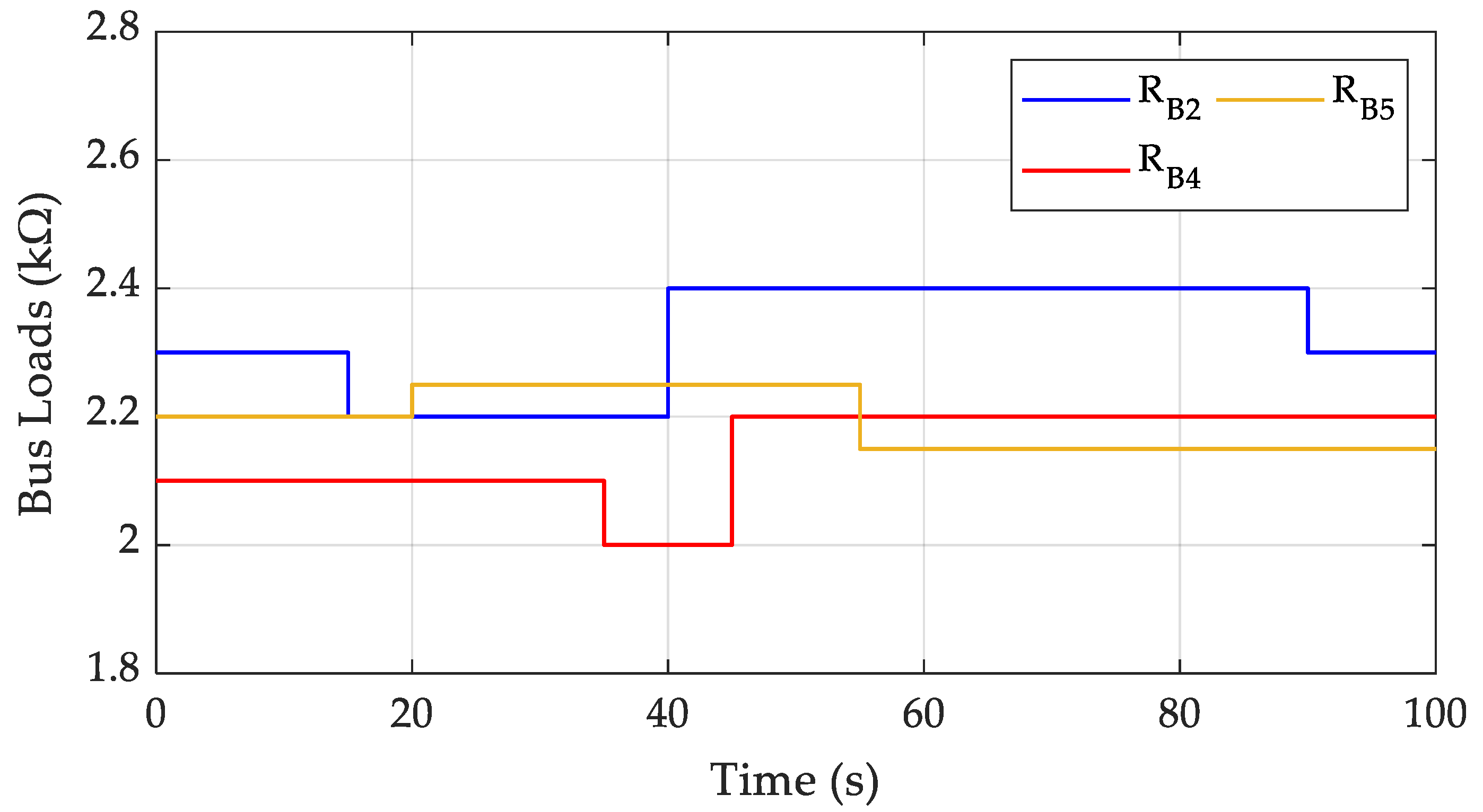
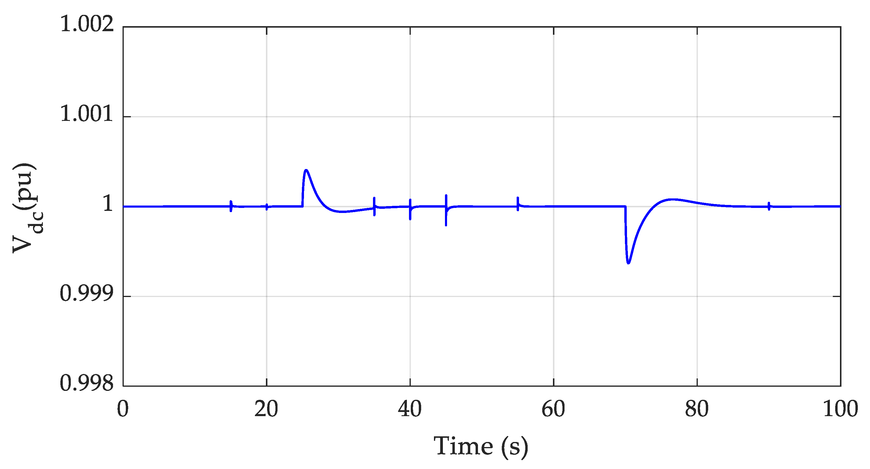
For the admittance part of the CIAT formulation

$$\tilde{M}=diag\left\{C_{B1},C_{B1},C_{B2},C_{B2},C_{B3},C_{B3},C_{B4},C_{B4},C_{B5},C_{B5},\frac{2}{3}{C}_{dc}\right\},$$

$$\tilde{D}=diag\left\{\frac{1}{R_{B1}},\frac{1}{R_{B1}},\frac{1}{R_{B2}},\frac{1}{R_{B2}},\frac{1}{R_{B3}},\frac{1}{R_{B3}},\frac{1}{R_{B4}},\frac{1}{R_{B4}},\frac{1}{R_{B5}},\frac{1}{R_{B5}},R_{dc}\right\}\hspace{0.17em}\mathrm{and}$$

$$\tilde{J}=\left[\begin{array}{ccc}\begin{array}{cc}0& w_s{C}_{B1}\\ -w_s{C}_{B1}& 0\end{array}& 0^{2\times 1}& 0^{2\times 8}\\ 0^{2\times 2}& \begin{array}{cc}0& w_s{C}_{B2}\\ -w_s{C}_{B2}& 0\end{array}& 0^{2\times 7}\\ 0^{2\times 4}& \begin{array}{cc}0& w_s{C}_{B3}\\ -w_s{C}_{B3}& 0\end{array}& 0^{2\times 5}\\ 0^{2\times 6}& \begin{array}{cc}0& w_s{C}_{B4}\\ -w_s{C}_{B4}& 0\end{array}& 0^{2\times 3}\\ 0^{2\times 8}& \begin{array}{cc}0& w_s{C}_{B5}\\ -w_s{C}_{B5}& 0\end{array}& 0^{2\times 1}\\ 0& 0& 0^{1\times 9}\end{array}\right],$$

3.

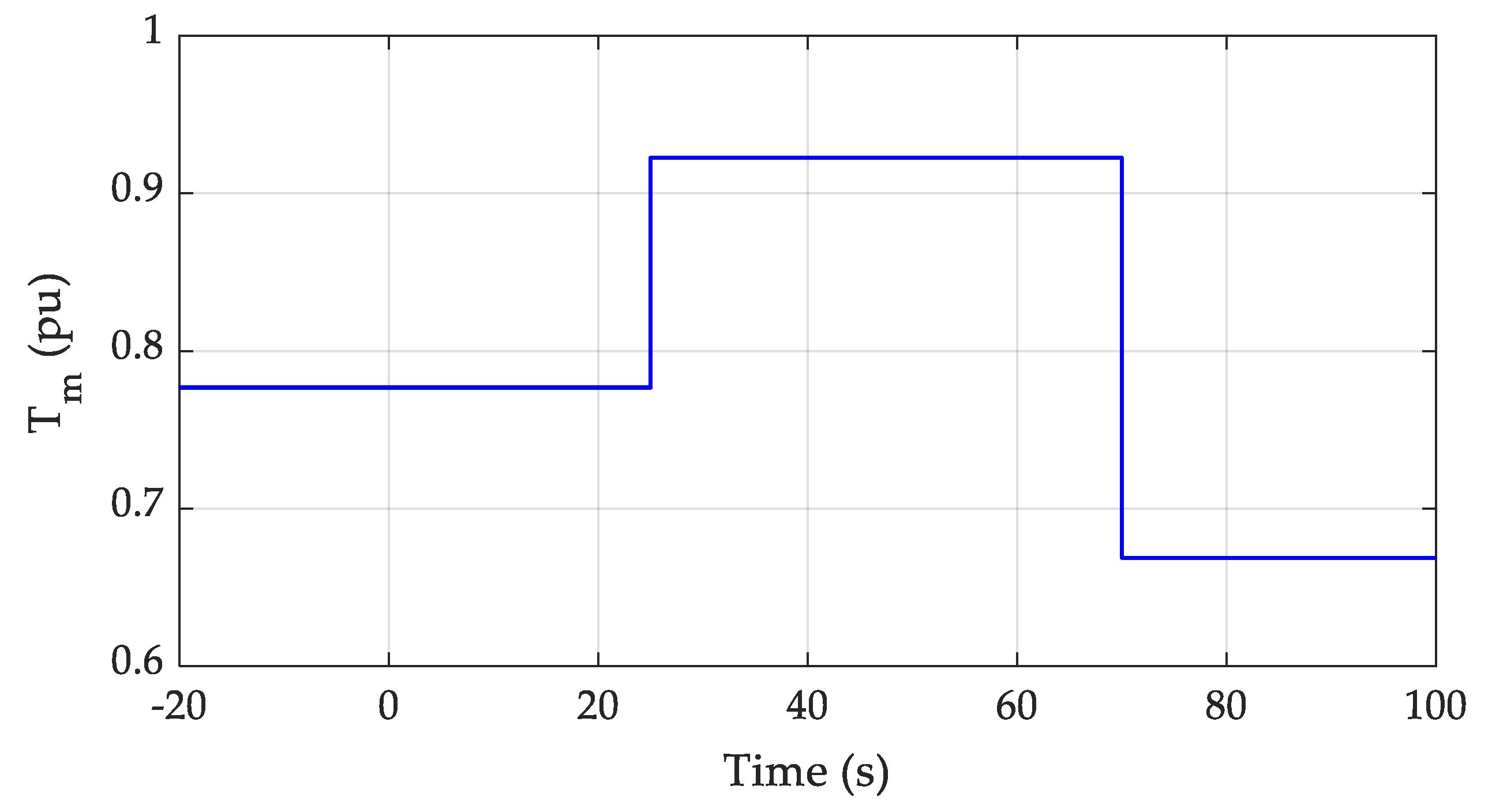
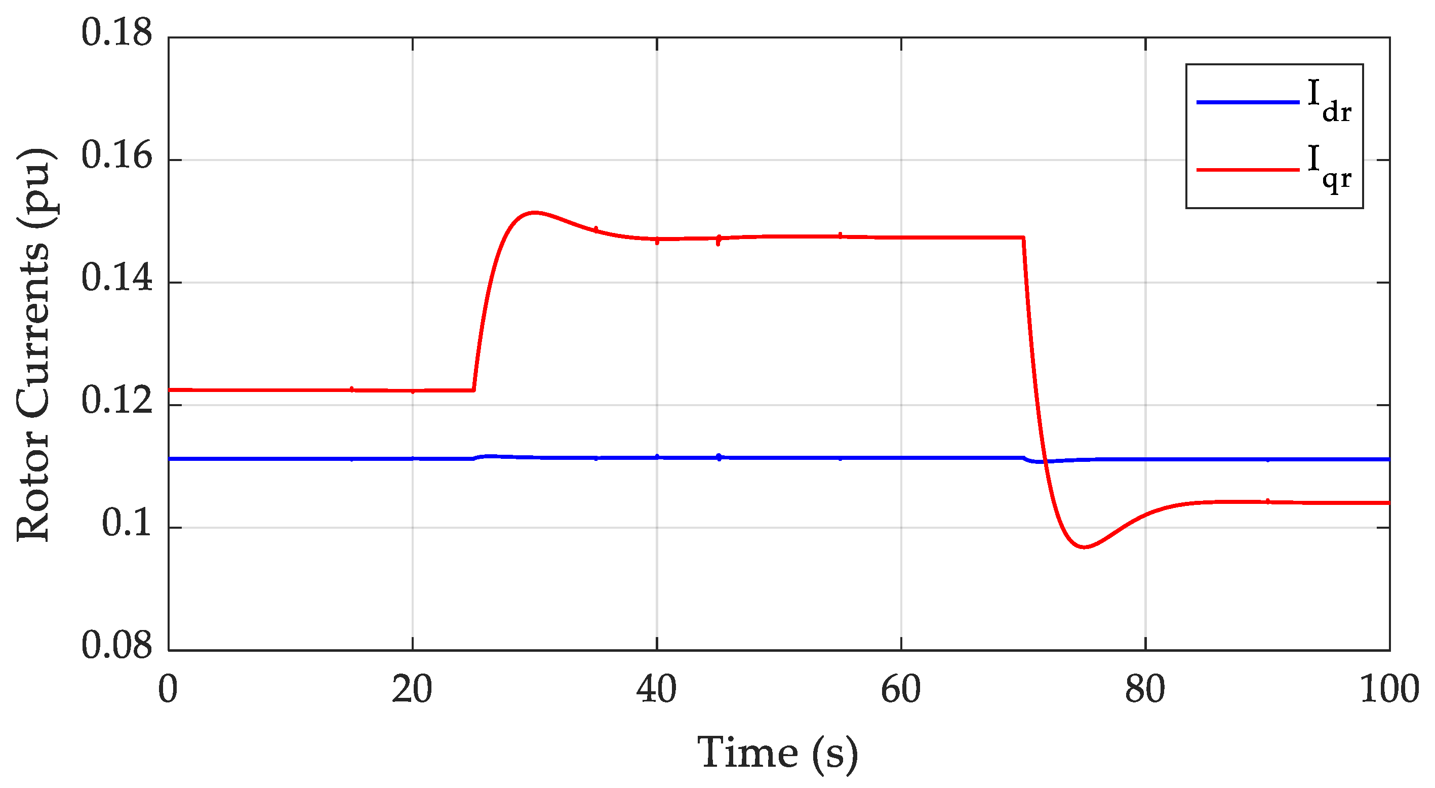
For the torque part of the CIAT formulation

$H=\left[\frac{2}{3}{H}_m\right]$ and $\overline{D}=\left[\frac{2}{3}b\right]$, where $H_m$ represents the total combined inertia of the WRIG rotor and the wind turbine, whereas b defines the rotor friction coefficient.

A simple inspection of the above matrices is adequate to immediately verify that both features, the one of Property 1 concerning the original IA formulation and the expanded ones stated in Property 2 are absolutely retained and thus, the resulting CIAT model is completely valid. It is easily seen from the model structure that it declares a fully damped system. Therefore, in accordance to the analysis presented in the previous section, the stability of the examined system is automatically guaranteed. Specifically, the results of Theorem 1 regarding fully damped systems can be directly applied so as to provide the desired global state converging properties.

Nevertheless, in order to demonstrate the generality in applying the CIAT modeling approach and its capability to describe many power system structures, a slightly different case is considered. In particular, it is assumed that the last term of diagonal damping matrix $\tilde{D}$ is zero, resulting when the parasitic resistance, $R_{dc}$, in parallel with the dc-link capacitor is neglected, a fact certainly considered in such dc-links. Obviously, the system is now characterized as a partially damped one, and, in accordance to the discussed procedure of analysis in Section 3, the following reformation is made for the state vector:

$$x^T=\left[\begin{array}{cc}{x}_1& ⋮x_2\end{array}\right]=\left[\begin{array}{ccccc}i& v_1& w_r& ⋮& v_{dc}\end{array}\right]$$

(25)

where now $v_1^T=\left[\begin{array}{cccccccccc}{v}_{dB1}& v_{qB1}& v_{dB2}& v_{qB2}& v_{dB3}& v_{qB3}& v_{dB4}& v_{qB4}& v_{dB5}& v_{qB5}\end{array}\right]$, and an input vector $u^T=\left[\begin{array}{cc}{u}_1& ⋮u_2\end{array}\right]=\left[\begin{array}{ccccc}V& I_1& -T_m& ⋮& 0\end{array}\right]$, with $I_1^T=\left[0^{1\times 10}\right]$ and the rest of the system matrices, i.e., $A(x)$ and $B(x)$ are obtained in accordance to formulation of Equation (22). By adopting this description, it can be easily proven that Assumptions 1 and 2 of Theorem 1 hold true and therefore, it can be directly applied in order to conclude again global state convergence to equilibrium.

The successful implementation of the CIAT modeling approach is expected to provide the advantages of accurate system dynamic performance evaluation by considering all its contributing subsystems and most importantly, of guaranteeing the complete system stable behavior, as long as the CIAT properties hold. In order to verify these results, an extensive simulation was conducted based on the deployed model provided in the previous subsection. The adopted parameters for modeling the DFIG subsystem were taken as in [37] and are presented in

Table 1. Single doubly fed induction generator (DFIG) system parameters.

Parameters/Values
$P_n=1.5 \mathrm{MW}$	$L_r=0.0053137 \mathrm{H}$	$n_g=62.5$
$V_s=700\mathrm{V}\left(\mathrm{rms}\right)$	$L_m=0.0051839 \mathrm{H}$	$R_T=30 \mathrm{m}$
$R_s=0.01 \mathsf{\Omega }$	$p=3$	$R_f=0.04 \mathsf{\Omega }$
$R_r=0.00842 \mathsf{\Omega }$	$b=0.00015\mathrm{N}\cdot \mathrm{m}\cdot \mathrm{s}/\mathrm{rad}$	$L_f=0.008 \mathrm{H}$
$L_s=0.005305 \mathrm{H}$	$H_m=765\mathrm{kg}\cdot {\mathrm{m}}^2$	$C_{dc}=0.02 \mathrm{F}$

, while the parameters chosen for implementing the MV grid layout are defined in

Table 2. Medium voltage (MV) grid parameters.

Parameters/Values
$R_{lkj}=12.5 \mathsf{\Omega }$	$R_{B3}=2.2 \mathrm{k}\mathsf{\Omega }$
$L_{lkj}=50 \mathrm{mH}$	$n=35.71$
$C_{Bi}=240 \mathrm{nF}$	$k=6$
$R_{B1}=1.4 \mathrm{k}\mathsf{\Omega }$	$f=50 \mathrm{Hz}$

.

The simulation scenario features step changes in the external input of the mechanical torque applied on the WRIG rotor, $T_m$, as illustrated in Figure 2, which actually correspond to variations of the wind speed acting on the wind turbine. Additionally, several abrupt variations of the local grid loads, are described graphically in Figure 3, representing rapid changes in the load power demands. It should be noted that these rather large and rapid variations were considered such as to stress the system as much as possible, aiming to validate its satisfactory performance under tight conditions.

According to this concept, the dynamic response of the system is presented in Figure 4, Figure 5, Figure 6, Figure 7, Figure 8, Figure 9 and Figure 10 in the per unit system representation by considering a total apparent power base of $S_b=$4 × 1.66 MWA, and voltage bases of 700 V and 25 kV for the wind farm and for the local grid layout parts, respectively. Additionally, the voltage base for the HV transmission part of the system was selected at 150 kV. In particular, Figure 4 depicts the rotor d-q current components of a single DFIG-based wind turbine, while in Figure 5 the respective current components for the stator and GSC are illustrated. One can observe that the generator currents mostly change in response to variations of the external torque applied on the rotor, while they remain virtually unaffected by changes in grid loads. The generator current state trajectories reach their corresponding equilibrium without any large overshoots exhibiting an all-around stable behavior.

A similar conclusion can be deducted by examining Figure 6, where the voltage at the dc-link is presented. Since a large part of the power provided by the DFIG to the grid is transferred through the dc-link, it is absolutely desirable to maintain the dc-link voltage inside well-defined limits in order to avoid large power variations. Indeed, it is observed that the dc-link voltage presents only small deviations from its nominal value and mostly at times when the external mechanical torque input varies, thus ensuring seamless power transfer.

The stable behavior of the system is once again verified, by inspecting Figure 7 and Figure 8. Specifically, Figure 7 and Figure 8 illustrate the bus voltage magnitudes for the five buses of the system and the line current magnitudes flowing between them, respectively. It is important to notice that the bus voltages remain well within the technically acceptable range of operation, as they tend very close to their nominal value in all cases. Additionally, the line current magnitudes exhibit a stable response as well, displaying variations depending on the load demand and the required power transfer conditions.

Regarding these power flow conditions, Figure 9 demonstrates the total active power provided by the wind farm, whereas Figure 10 depicts the active power flowing through the lines of the MV local grid. According to the considered simulation scenario, the rapid change in the mechanical torque applied on the rotors of the DFIG-based wind turbines at t = 25 s results in a reverse of power flow since the wind farm at this time operates closely to its nominal conditions, which in turn results in feeding the additional power to the main HV grid. Conversely, when the external mechanical torque is abruptly reduced at t = 70 s, it is observed that some of the MV grid loads need to be fed by the HV main power grid.

In general, all results obtained through the simulation of the considered system-example highlight the significant advantages that the proposed modeling approach can provide. The CIAT formulation itself allows a complete and comprehensive examination of dynamics deriving from many different components that coexist in the given power structure, while simultaneously, the remarkable properties accompanying the CIAT formulation automatically ensure strong stability conditions for the complete system, in accordance to the results of Section 3.

5. Conclusions

A novel modeling approach is developed, introduced as CIAT formulation, which offers the notable advantage of including dynamics deriving from all subsystems comprising any considered grid layout in modern power systems. The proposed holistic method leads to a complete and precise generalized nonlinear description that holds a common structure with generic fundamental properties, while simultaneously it enables the direct stability verification of any examined layout that satisfies the respective properties. Given this accurate representation, it becomes possible to automatically establish and verify strong stability conditions for any kind of power system just by inspecting it for fulfilling the basic properties of the CIAT description. In this frame, two fundamental Theorems are proven to realize strong stability conditions for any system following the CIAT model, which are further specialized to the establishment of state-converging properties that hold globally or in a specific RoA under some mild conditions. A main contribution of the present work is that it is based on the most possible accurate system and components models (from the grid lines to the power converters and electric machines) under a new view that does not neglect the inherent system nonlinearities. To demonstrate and verify this remarkable feature, a modern DG-based power system example is deployed as CIAT model. It is therefore verified that although a large-scale system is handled, its stability properties are immediately observed from the system structure and are additionally evaluated by extended simulations. Indeed, the extracted response results reveal a clearly efficient, stable, and satisfactory dynamic performance of the system, in full compliance with the theoretical claims.

References

1. Jiayi, H.; Chuanwen, J.; Rong, X. A review on distributed energy resources and MicroGrid. Renew. Sustain. Energy Rev. 2008, 12, 2472–2483. [Google Scholar] [CrossRef]
2. Fang, J.; Li, H.; Tang, Y.; Blaabjerg, F. On the Inertia of Future More-Electronics Power Systems. IEEE J. Emerg. Sel. Top. Power Electron. 2019, 7, 2130–2146. [Google Scholar] [CrossRef]
3. Olivares, D.E.; Mehrizi-Sani, A.; Etemadi, A.H.; Canizares, C.A.; Iravani, R.; Kazerani, M. Trends in Microgrid Control. IEEE Trans. Smart Grid 2014, 5, 1905–1919. [Google Scholar] [CrossRef]
4. Spanias, C.; Lestas, I. A System Reference Frame Approach for Stability Analysis and Control of Power Grids. IEEE Trans. Power Syst. 2019, 34, 1105–1115. [Google Scholar] [CrossRef]
5. Pagani, G.A.; Aiello, M. The Power Grid as a complex network: A survey. Phys. A Stat. Mech. Its Appl. 2013, 392, 2688–2700. [Google Scholar] [CrossRef] [Green Version]
6. Faloutsos, M.; Faloutsos, P.; Faloutsos, C. On power-law relationships of the internet topology. In Proceedings of the Conference on Applications, Technologies, Architectures, and Protocols for Computer Communication; ACM: Cambridge, MA, USA, August 1999; p. 262. [Google Scholar]
7. Albert, R.; Jeong, H.; Barabási, A.L. Internet: Diameter of the World-Wide Web. Nature 1999, 401, 130–131. [Google Scholar] [CrossRef] [Green Version]
8. Boss, M.; Elsinger, H.; Summer, M.; Thurner, S. The network topology of the interbank market. Quant. Financ. 2004, 4, 677–684. [Google Scholar] [CrossRef]
9. Yang, C.; Guan, Z.H.; Liu, Z.W.; Chen, J.; Chi, M.; Zheng, G.-L. Wide-area multiple line-outages detection in power complex networks. Electr. Power Energy Syst. 2016, 79, 132–141. [Google Scholar] [CrossRef]
10. Arianos, S.; Bompard, E.; Carbone, A.; Xue, F. Power grid vulnerability: A complex network approach. CHAOS 2009, 19, 1–6. [Google Scholar] [CrossRef]
11. Papageorgiou, P.C.; Alexandridis, A.T. A suitable to the microgrid analysis approach for nonlinear modeling and control of an inverter interface. In Proceedings of the 25th Mediterranean Conference on Control and Automation (MED-2017), Valletta, Malta, 3–6 July 2017; pp. 522–527. [Google Scholar]
12. Fiaz, S.; Zonetti, D.; Ortega, R.; Scherpen, J.M.A.; van der Schaft, A.J. A port-Hamiltonian approach to power network modeling and analysis. Eur. J. Control 2013, 19, 477–485. [Google Scholar] [CrossRef]
13. Konstantopoulos, G.C.; Alexandridis, A.T. Generalized nonlinear stabilizing controllers for Hamiltonian passive systems with switching devices. IEEE Trans. Control Syst. Technol. 2013, 21, 1479–1488. [Google Scholar] [CrossRef]
14. Kundur, P. Power System Stability and Control; McGraw-Hill: New York, NY, USA, 1994. [Google Scholar]
15. Vu, T.L.; Turitsyn, K. Lyapunov functions family approach to transient stability assessment. IEEE Trans. Power Syst. 2016, 31, 1269–1277. [Google Scholar] [CrossRef] [Green Version]
16. Slotine, J.-J.E.; Li, W. Applied Nonlinear Control, 1st ed.; Prentice-Hall: Englewood Cliffs, NJ, USA, 1991. [Google Scholar]
17. Ortega, R.; Loría Perez, J.A.; Nicklasson, P.J.; Sira-Ramirez, H. Passivity-Based Control of Euler-Lagrange Systems, 1st ed.; Springer: London, UK, 1998. [Google Scholar]
18. Watson, J.; Ojo, Y.; Lestas, I.; Spanias, C. Stability of power networks with grid-forming converters. In Proceedings of the 2019 IEEE Milan PowerTech, Milan, Italy, 23–27 June 2019; pp. 1–6. [Google Scholar]
19. Ghandhari, M.; Andersson, G.; Hiskens, I.A. Control Lyapunov functions for controllable series devices. IEEE Trans. Power Syst. 2001, 16, 689–694. [Google Scholar] [CrossRef]
20. Alexandridis, A.T.; Papageorgiou, P.C. A complex network deployment suitable for modern power distribution analysis at the primary control level. IFAC-PapersOnLine 2017, 50, 9186–9191. [Google Scholar] [CrossRef]
21. Alexandridis, A.T. Studying State Convergence of Input-to-State Stable Systems with Applications to Power System Analysis. Energies 2020, 13, 92. [Google Scholar] [CrossRef] [Green Version]
22. Berger, T.; Halikias, G.; Karcanias, N. Effects on dynamic and non-dynamic element changes in RC and RL networks. Int. J. Circuit Theory Appl. 2015, 43, 36–59. [Google Scholar] [CrossRef] [Green Version]
23. Glover, J.D.; Sarma, M.S.; Overbye, T.T. Power System Analysis & Design, 5th ed.; Cengage Learning, 200 First Stamford Place: Stamford, CT, USA, 2012. [Google Scholar]
24. Krause, P.C.; Wasynczuk, O.; Sudhoff, S.D. Analysis of Electric Machinery and Drive Systems, 2nd ed.; Wiley-IEEE Press: Piscataway, NJ, USA, 2002. [Google Scholar]
25. Wang, B.; Cai, G.; Yang, D.; Wang, L.; Yu, Z. Investigation on Dynamic Response of Grid-Tied VSC During Electromechanical Oscillations of Power Systems. Energies 2020, 13, 94. [Google Scholar] [CrossRef] [Green Version]
26. Krein, P.T.; Bentsman, J.; Bass, R.M.; Lesieutre, B.L. On the Use of Averaging for the Analysis of Power Electronic Systems. IEEE Trans. Power Electron. 1990, 5, 182–190. [Google Scholar] [CrossRef]
27. Sira-Ramirez, H.; Silva-Ortigoza, R. Control Design Techniques in Power Electronics Devices; Springer: London, UK, 2006. [Google Scholar]
28. Yazdani, A.; Iravani, R. Voltage-Sourced Converters in Power Systems; Wiley Press: Hoboken, NJ, USA, 2010. [Google Scholar]
29. Kundur, P.; Paserba, J.; Ajjarapu, V.; Andersson, G.; Bose, A.; Canizares, C.; Hatziargyriou, N.; Hill, D.; Stankovic, A.; Taylor, C.; et al. Definition and classification of power system stability IEEE/CIGRE joint task force on stability terms and definitions. IEEE Trans. Power Syst. 2004, 19, 1387–1401. [Google Scholar]
30. Marquez, H.J. Nonlinear Control Systems; Wiley & Sons, Inc.: Hoboken, NJ, USA, 2003. [Google Scholar]
31. Sontag, E.D.; Wang, Y. New characterizations of input-to-state stability. IEEE Trans. Autom. Control 1996, 41, 1283–1294. [Google Scholar] [CrossRef] [Green Version]
32. Khalil, H.K. Nonlinear Systems, 3rd ed.; Prentice-Hall: Upper Saddle River, NJ, USA, 2002. [Google Scholar]
33. Sontag, E.D. Input to state stability: Basic concepts and results. In Nonlinear and Optimal Control Theory. Lecture Notes in Mathematics, 1st ed.; Nistri, P., Stefani, G., Eds.; Springer: Berlin, Germany, 2008; Volume 1932, pp. 163–220. [Google Scholar]
34. Konstantopoulos, G.C.; Alexandridis, A.T. Stability and convergence analysis for a class of nonlinear passive systems. In Proceedings of the 50th Conference on Decision and Control and European. Control Conference (CDC-ECC), Orlando, FL, USA, 12–15 December 2011; pp. 1753–1758. [Google Scholar]
35. Panteley, E.; Loria, A.; Teel, A. Relaxed persistency of excitation for uniform asymptotic stability. IEEE Trans. Autom. Control 2001, 46, 1874–1886. [Google Scholar] [CrossRef]
36. Loria, A.; Panteley, E.; Teel, A. A new persistency of excitation condition for UGAS of NLTV systems: Application to stabilization of nonholonomic systems. In Proceedings of the 5th European Control Conference, Karlsruhe, Germany, 31 August–3 September 1991. Paper No. 500. [Google Scholar]
37. Bourdoulis, M.K.; Alexandridis, A.T. Direct Power Control of DFIG Wind Systems Based on Nonlinear Modeling and Analysis. IEEE J. Emerg. Sel. Top. Power Electron. 2014, 2, 764–775. [Google Scholar] [CrossRef]
Figure 1. One-line diagram of considered distributed generation (DG)-based power system.
Energies 13 02461 g001
Figure 2. Magnitude of mechanical torque applied on the wound rotor induction generator (WRIG) rotor.
Energies 13 02461 g002
Figure 3. Step changes in local ohmic bus loads.
Energies 13 02461 g003
Figure 4. Rotor d- and q-axis components.
Energies 13 02461 g004
Figure 5. Stator and grid-side converter (GSC) d- and q-axis components.
Energies 13 02461 g005
Figure 6. Voltage at the dc-link.
Energies 13 02461 g006
Figure 7. Local bus voltage magnitudes.
Energies 13 02461 g007
Figure 8. Line current magnitudes.
Energies 13 02461 g008
Figure 9. Wind farm active power output.
Energies 13 02461 g009
Figure 10. Active power flowing in local grid lines.
Energies 13 02461 g010