Coordinated Excitation and Static Var Compensator Control with Delayed Feedback Measurements in SGIB Power Systems

Abstract

In this paper, we present a nonlinear coordinated excitation and static var compensator (SVC) control for regulating the output voltage and improving the transient stability of a synchronous generator infinite bus (SGIB) power system. In the first stage, advanced nonlinear methods are applied to regulate the SVC susceptance in a manner that can potentially improve the overall transient performance and stability. However, as distant from the generator measurements are needed, time delays are expected in the control loop. This fact substantially complicates the whole design. Therefore, a novel design is proposed that uses backstepping methodologies and feedback linearization techniques suitably modified to take into account the delayed measurement feedback laws in order to implement both the excitation voltage and the SVC compensator input. A detailed and rigorous Lyapunov stability analysis reveals that if the time delays do not exceed some specific limits, then all closed-loop signals remain bounded and the frequency deviations are effectively regulated to approach zero. Applying this control scheme, output voltage changes occur after the large power angle deviations have been eliminated. The scheme is thus completed, in a second stage, by a soft-switching mechanism employed on a classical proportional integral (PI) PI voltage controller acting on the excitation loop when the frequency deviations tend to zero in order to smoothly recover the output voltage level at its nominal value. Detailed simulation studies verify the effectiveness of the proposed design approach.

1. Introduction

Power systems are nonlinear, large-scale, widely dispersed systems with many different interconnected components. Typically, power systems controls are structured in several hierarchical levels (primary, secondary, tertiary). The primary level control of power systems plays a central role in maintaining transient stability and obtaining a desired system performance. Generator excitation control is employed at the primary level in order to improve the power system stability, especially after short-circuit faults or other major disturbances. This is achieved with the use of supplementary excitation control devices called power systems stabilizers (PSSs). Conventional PSS are designed using linear control approaches and are combined with the automatic voltage regulator (AVR) part to result in a common form, known as an AVR/PSS controller. In the case of a synchronous generator infinite bus (SGIB) power system, linear excitation controllers have been proposed in [1], which are based on linearizations around the operating point. Nonlinear control theory, on the other hand, seems to provide a more reliable and robust tool for the analysis and design of power systems [2]. Under this view, several nonlinear excitation control methods have been proposed including feedback linearization [3,4], adaptive control [4,5,6,7], and robust designs [8,9].

Beyond the traditional control of power systems through the excitation circuits of the rotating generators, static power-electronic devices are proposed to be installed in the power transmission system to support their transient behavior. Such static power-electronic components are the flexible alternating current transmission system (FACTS) devices that are suitably controlled to increase the power transfer capability and network stability [10,11]. Static var compensators (SVCs) are FACTS devices that correct the power factor and the grid voltage at the point of connection [12,13,14]. In this paper, we consider a widely used thyristor controlled reactor-fixed capacitor (TCR-FC) SVC [15,16]. Voltage is regulated at the SVC bus as follows: If voltage amplitude is needed to decrease (i.e., in case of capacitive load conditions), the SVC uses TCRs to absorb vars from the system. If voltage amplitude is needed to increase (in case of inductive load conditions), the capacitor banks are automatically switched-in to inject vars to the system. In several studies [12,13,14,15,16,17,18,19], coordinated excitation and SVC control has been considered for transient stability enhancement and voltage regulation.

Recent advances in wide-area measurement systems (WAMS) technology have initiated the use of phasor measurement unit (PMU) devices for controlling power systems. Communication time-delays are inevitably introduced during the transmission of wide-area signals. The effect of these delays on the overall power system stability has attracted significant research interest [20,21] because they constitute additionally negative factors in designing an effective control.

In this paper, we consider a single machine infinite bus power system with a TCR-FC SVC connected in the tie-lines between the generator and the infinite bus. The synchronous generator is represented by its third-order nonlinear model and the SVC dynamics from its first-order model. A feedback linearization approach is used, resulting in a linear dynamic system representation with two controlled inputs, the generator excitation input and the input of the SVC regulator. Both inputs are used in conjunction to formulate a faster and effective feedback loop that can substantially improve the overall system transient response and stability. Applying backstepping-based techniques and using distant measurements from the generator side, an excitation and a nonlinear SVC controller are designed. As the time delays in the measurements are essential for the whole design, a detailed nonlinear theoretical analysis is conducted that considers this influence and, as shown in the paper, proves that as long as the time delays are sufficiently small, then all closed-loop signals are bounded and the power angle deviations exponentially converge to zero. The design is completed by a coordinated frequency and voltage controller that utilizes a soft switching mechanism for both the excitation input and the SVC compensator, which extends the fuzzy switching coordination approach of [22]. The excitation input initially employs the proposed nonlinear control, while in the sequel, after the large frequency deviations are mitigated, it switches in a smooth way to a classical automatic voltage regulator and power system stabilizer (AVR/PSS). It is apparent that also in the case when the delays are not sufficiently small, then a classical proportional integral (PI) voltage controller is used. The simulation results indicate that the proposed approach yields better results than the simple AVR/PSS and PI SVC control.

The main contributions and novelties of this work with respect to the related literature [13,14,15,16,17,18,19,22] are summarized as follows:

• This work is the first to consider the use of SVC control laws with delayed measurements from the generator in order to improve the overall transient stability and performance. The proposed approach makes necessary a new theoretical analysis that takes into account the effect of time-delays.
• The soft switching coordination approach of [22], which improves global transient stability and voltage regulation, is extended to the SVC control case. New membership functions are considered based on suitably defined fuzzy rules that consider not only the frequency variations, but also the magnitude of the time delays.

The rest of the paper is organized as follows. In Section 2, the mathematic model of the system is outlined and the problem is formulated. The backstepping/feedback linearization method is used in Section 3 to design the excitation and SVC controllers. In Section 4, a detailed stability analysis for the closed-loop system is carried out. The coordinated frequency and voltage control is proposed in Section 5. Simulation results are given in Section 6. Finally, in Section 7, some concluding remarks are given.

2. Mathematical Model and Problem Formulation

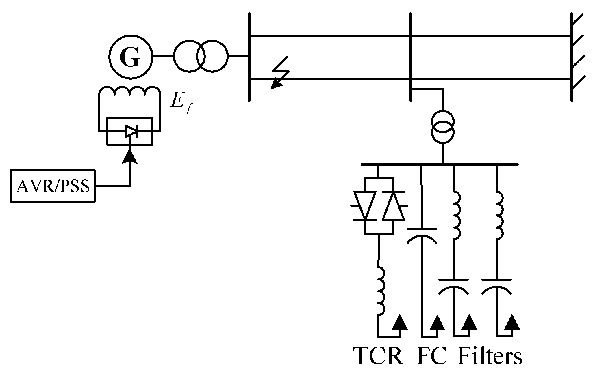
A simplified model for a generator and an SVC system, which forms a three-bus system shown in Figure 1, is considered. The SVC is connected to a bus located at an intermediate point of the transmission line.

The classical third-order single-axis dynamic generator model [23] is used for the design of the excitation controller, which neglects dynamics with very short time constants, and is given by the following equations:

$$\dot{\delta }\left(t\right)=\omega \left(t\right)-{\omega }_0$$

(1)

$$\dot{\omega }\left(t\right)=-\frac{D}{M}\left(\omega \left(t\right)-{\omega }_0\right)+\frac{{\omega }_0}{M}\left(P_m-P_e\left(t\right)\right)$$

(2)

$${\dot{E}}_q^{\prime }\left(t\right)=\frac{1}{T_{d0}^{\prime }}\left(E_f\left(t\right)-E_q\left(t\right)\right)$$

(3)

where

$$E_q\left(t\right)=E_q^{\prime }\left(t\right)+\left(x_d-x_d^{\prime }\right)I_d\left(t\right)$$

(4)

$$E_f\left(t\right)=k_c{u}_f\left(t\right)$$

(5)

In this model, the sub-transient and damper windings effects are neglected. Moreover, the flow terms ${\dot{\lambda }}_d$ and ${\dot{\lambda }}_q$ in the stator voltage equations are omitted as they are considered negligible compared with the speed voltage terms.

We consider a widely used TCR-FC SVC (see Figure 1), which consists of a fixed capacitor in shunt with a thyristor-controlled inductor. Let $B_C$ be the susceptance of the capacitor in SVC and $B_L(t)$ be the susceptance of the inductor in SVC. Let it be that $B_L(t)$ is regulated by the firing angle of the thyristor. Then, the equivalent dynamic model of SVC can be written as [15,16,17]

$${\dot{B}}_L\left(t\right)=\frac{1}{T_B\left(t\right)}\left(-B_L\left(t\right)+B_{L0}+k_B{u}_B\left(t\right)\right)$$

(6)

where $B_{L0}$ is the initial susceptance of the TCR, $T_B$ is the time constant of the SVC regulator, $k_B$ the gain, and $u_B$ the input of the SVC regulator.

The coordinated control design for the generator and the static VAR compensator must take into account the SVC controller effect on the generator dynamics. From the network topology depicted in Figure 1, the active electrical power is given by

$$P_e=\frac{E_q^{\prime }\sin \delta }{X}$$

(7)

where $X$ is the total reactance value.

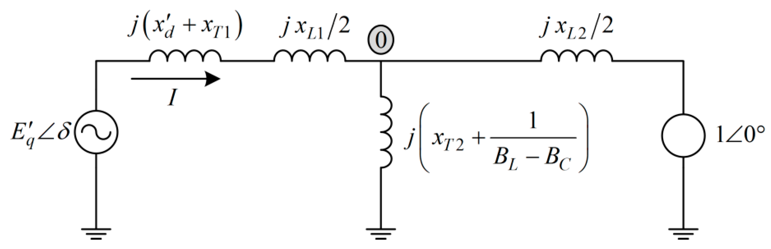
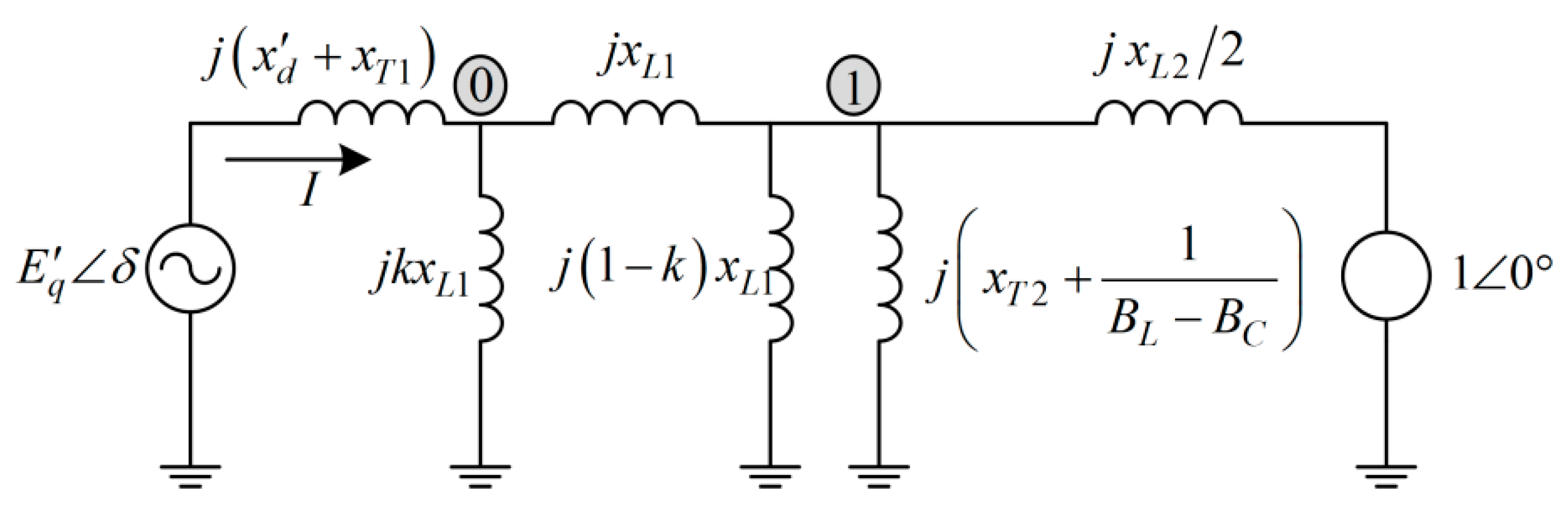
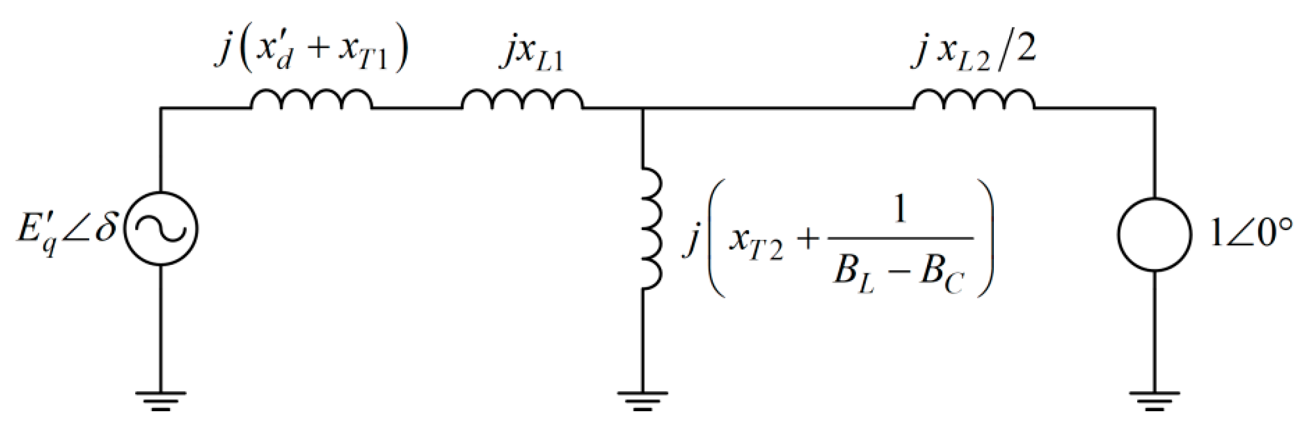
To examine the transient system response, a symmetrical three-phase short-circuit fault in the tie-line connecting the generator and the static VAR compensator is considered, as shown in Figure 1. During the three-phase short-circuit fault, the total reactance value Χ changes. An analysis of the equivalent circuits pre-fault, during fault, and post-fault yields the respective values of $X$. These network configurations are shown in Figure 2, Figure 3 and Figure 4, whereas the detailed calculations are given in Appendix A.

Specifically, the total reactance value $X$ before the fault is

$$X=x_d^{\prime }+x_{T1}+\frac{x_{L1}}{2}+\frac{x_{L2}}{2}+\frac{x_{L2}}{2}\left(x_d^{\prime }+x_{T1}+\frac{x_{L1}}{2}\right){\left(x_{T2}+\frac{1}{B_L-B_C}\right)}^{-1}.$$

(8)

During the fault, the total reactance is changed to

$$\begin{array}{l}X=\left[\frac{x_{L1}{x}_{L2}}{2}+\frac{\left(k+1\right)x_{L2}}{2k}\left(x_d^{\prime }+x_{T1}\right)\right]\times \\ \times \left[\frac{2}{x_{L2}}+\frac{2-k}{\left(1-k\right)x_{L1}}-\frac{1}{x_{L1}^2}{\left(\frac{1}{x_d^{\prime }+x_{T1}}+\frac{1}{\frac{k}{k+1}{x}_{L1}}\right)}^{-1}+{\left(x_{T2}+\frac{1}{B_L-B_C}\right)}^{-1}\right].\end{array}$$

(9)

The constant $k\in \left(0,1\right)$ is determined by the fault position in the line between the generator bus and the SVC bus. The smaller $k$ is, the closer the the fault is to the generator bus. If $k$ is close to one, then the fault position is close to the SVC bus, whereas $k=0.5$ denotes a fault at the middle of this line.

After the fault is removed (by opening the brakers), it takes the following form:

$$X=x_d^{\prime }+x_{T1}+x_{L1}+\frac{x_{L2}}{2}+\frac{x_{L2}}{2}\left(x_d^{\prime }+x_{T1}+x_{L1}\right){\left(x_{T2}+\frac{1}{B_L-B_C}\right)}^{-1}$$

(10)

To proceed with the control design, we differentiate (7) to obtain the rate of change of $P_e$ as

$$\frac{d{P}_e\left(t\right)}{dt}=\frac{E_q^{\prime }\cos \delta }{X}\Delta \omega +\frac{d{E}_q^{\prime }}{dt}\frac{\sin \delta }{X}-\frac{1}{X}{P}_e\frac{dX}{dt}$$

(11)

Considering (8)–(10), the time derivative of $X$ for the three different modes can be computed as

$$\frac{dX\left(t\right)}{dt}=\frac{a}{{\left[x_{T2}\left(B_L\left(t\right)-B_C\right)+1\right]}^2}\frac{d{B}_L\left(t\right)}{dt}$$

(12)

where $a$ is a constant with the following values:

$$a=\{\begin{array}{c}\frac{x_{L2}}{2}\left(x_d^{\prime }+x_{T1}+\frac{x_{L1}}{2}\right),beforefault\\ \frac{x_{L2}}{2}\left[x_{L1}+\left(1+1/k\right)\left(x_d^{\prime }+x_{T1}\right)\right],duringfault\\ \frac{x_{L2}}{2}\left(x_d^{\prime }+x_{T1}+x_{L1}\right),afterfault\end{array}.$$

(13)

Expressions (11), (12), and (13) are used in the following design procedure.

3. Control Design Based on Backstepping and Feedback Linearization Techniques

The control objective is to design the excitation input $E_f$ and the SVC controller $u_B$ such that the angle deviations $\Delta \delta$ converge exponentially fast to zero. To that end, we adopt a backstepping approach in the control design for the transient stability enhancement similar to [3]. Let the first error variable be $z_1=\Delta \delta$ with dynamics ${\dot{z}}_1=\Delta \omega$. If we define the first virtual control law ${\alpha }_1=-c_1\Delta \delta$ with $c_1>0$, then for the new error variable, $z_2=\Delta \omega -{\alpha }_1$, and the nonnegative function, $V_1=\left(1/2\right)z_1^2$, we have that ${\dot{V}}_1=-c_1{z}_1^2+z_1{z}_2$. The dynamics of $z_2$ are given by

$${\dot{z}}_2\left(t\right)=\left(c_1-\frac{D}{M}\right)\Delta \omega \left(t\right)-\frac{{\omega }_0}{M}\Delta P_e$$

(14)

If we select the second virtual control law as

$${\alpha }_2=\frac{M}{{\omega }_0}\left[\left(c_1-\frac{D}{M}\right)\Delta \omega +z_1+c_2{z}_2\right]$$

(15)

with the third error variable $z_3=\Delta P_e-{\alpha }_2$, then the dynamics of $z_2$ are ${\dot{z}}_2=-z_1-c_2{z}_2-\left({\omega }_0/M\right)z_3$. The overall error variable transformation is

$$\left[\begin{array}{c}{z}_1\\ z_2\\ z_3\end{array}\right]=\left[\begin{array}{ccc}1& 0& 0\\ c_1& 1& 0\\ -\frac{M}{{\omega }_0}\left(1+c_1{c}_2\right)& -\frac{M}{{\omega }_0}\left(c_1+c_2-\frac{D}{M}\right)& 1\end{array}\right]\left[\begin{array}{c}\Delta \delta \\ \Delta \omega \\ \Delta P_e\end{array}\right]$$

(16)

Then, the dynamics of the $z_3$ error variable are described by

$$\begin{array}{l}{\dot{z}}_3=\frac{E_q^{\prime }\cos \delta }{X}\Delta \omega +\frac{1}{{T^{\prime }}_{d0}}\left(E_f-E_q^{\prime }-\left(x_d-x_d^{\prime }\right)I_d\right)\frac{\sin \delta }{X}-\frac{a{P}_e\left(-B_L\left(t\right)+B_{L0}+k_B{u}_B\left(t\right)\right)}{T_B\left(t\right)X{\left[x_{T2}\left(B_L\left(t\right)-B_C\right)+1\right]}^2}\\ +\frac{M}{{\omega }_0}\left(c_1+c_2-\frac{D}{M}\right)\left(\frac{D}{M}\Delta \omega +\frac{{\omega }_0}{M}\Delta P_e\right)-\frac{M}{{\omega }_0}\left(1+c_1{c}_2\right)\Delta \omega \end{array}$$

(17)

where expressions (11) to (13) are taken into account.

We then select a nonlinear feedback linearizing excitation control law of the following form:

$$\begin{array}{l}{E}_f=E_{f,NC}=E_q^{\prime }+\left(x_d-x_d^{\prime }\right)I_d-\frac{T_{d0}^{\prime }{E}_q^{\prime }\Delta \omega }{\tan \delta }+\frac{T_{d0}^{\prime }{E}_q^{\prime }}{P_e}[\frac{M}{{\omega }_0}\left(1+c_1{c}_2\right)c_3\Delta \delta +\\ +\frac{M}{{\omega }_0}\left(1+c_1{c}_2+\left(c_3-\frac{D}{M}\right)\left(c_1+c_2-\frac{D}{M}\right)\right)\Delta \omega -\left(c_1+c_2+c_3-\frac{D}{M}\right)\Delta P_e]\end{array}$$

(18)

and SVC control law

$$u_{B,NC}\left(t\right)=\frac{1}{k_B}\left[B_L\left(t\right)-B_{L0}+\frac{c_B{T}_B{\left[x_{T2}\left(B_L\left(t\right)-B_C\right)+1\right]}^2}{P_e}{z}_3\left(t-\tau \left(t\right)\right)\right]$$

(19)

with gain $c_B>0$. It is noticed that in (19), the time delay inserted from the $z_3$ measurement and feedback denoted by $\tau \left(t\right)$ is taken into account, and the following delayed ODE is obtained:

$$\begin{array}{l}{\dot{z}}_3=-c_3{z}_3\left(t\right)-\frac{a{c}_B}{X}{z}_3\left(t-\tau \left(t\right)\right)\\ z_3\left(\theta \right)=\varphi \left(\theta \right),\forall \theta \in E_0\end{array}$$

(20)

where $\varphi :E_0\to R$ is a continuous initial function with bounded norm defined in

$$E_0=\left\{t\in R|\eta -\tau \left(\eta \right)\le 0,\eta \ge t_0\right\}$$

The delay $\tau \left(t\right)$ is assumed to be bounded with the bounded rate of change, that is, $\underset{\_}{\tau }\le \tau \left(t\right)\le \overline{\tau }$ and $\dot{\tau }\left(t\right)\le \eta$ for some $\underset{\_}{\tau },\overline{\tau },\eta >0$. The delayed term in (19) is the result of the fact that the variable $z_3\left(t\right)$ does not involve local SVC measurements, but uses distant, and thus delayed, measurements from the generator. Thus, at time $t$, the $z_3\left(t-\tau \left(t\right)\right)$ is available for use in the SVC controller.

4. Overall System Stability Analysis

An analysis will be carried out next to prove that, under certain conditions on the magnitude of the time-delay, the error variable $z_3$ converges exponentially fast to zero.

It is worth noting that all solutions of (20) are also solutions of

$${\dot{z}}_3\left(t\right)=-\left(c_3+\frac{a{c}_B}{X}\right)z_3\left(t\right)-\frac{a{c}_B}{X}{\displaystyle \underset{t-\tau }{\overset{t}{\int }}\left(c_3{z}_3\left(s\right)+\frac{a{c}_B}{X}{z}_3\left(s-\tau \left(s\right)\right)\right)ds}.$$

(21)

The solution of (21) is given by

$$z_3\left(t\right)=\exp \left[-\left(c_3+\frac{a{c}_B}{X}\right)t\right]\varphi \left(0\right)-\frac{a{c}_B}{X}{\displaystyle \underset{0}{\overset{t}{\int }}{e}^{-\left(c_3+\frac{a{c}_B}{X}\right)\left(t-\theta \right)}{\displaystyle \underset{\theta -\tau }{\overset{\theta }{\int }}\left(c_3{z}_3\left(s\right)+\frac{a{c}_B}{X}{z}_3\left(s-\tau \left(s\right)\right)\right)ds}d\theta }$$

(22)

which in turn yields

$$\begin{array}{l}\left|z_3\left(t\right)\right|\le \exp \left[-\left(c_3+\frac{a{c}_B}{X}\right)t\right]\underset{\theta \in {\mathrm{E}}_0}{\sup }\left|\varphi \left(\theta \right)\right|+\\ +\frac{a{c}_B}{X}{\displaystyle \underset{0}{\overset{t}{\int }}\exp \left[-\left(c_3+\frac{a{c}_B}{X}\right)\left(t-\theta \right)\right]{\displaystyle \underset{\theta -\tau \left(\theta \right)}{\overset{\theta }{\int }}\left(c_3\left|z_3\left(s\right)\right|+\frac{a{c}_B}{X}\left|z_3\left(s-\tau \left(s\right)\right)\right|\right)ds}d\theta }.\end{array}$$

(23)

Consider now the functional differential equation

$$\dot{y}\left(t\right)=-\left(c_3+\frac{a{c}_B}{X}\right)y\left(t\right)+q\left(t\right)y\left(t-\tau \left(t\right)\right)$$

(24)

where

$$q\left(t\right)=\left(c_3+\frac{a{c}_B}{X}-\frac{\sigma }{\tau \left(t\right)}\right)\exp \left(-\sigma {\displaystyle \underset{t-\tau \left(t\right)}{\overset{t}{\int }}\frac{d\theta }{\tau \left(\theta \right)}}\right)$$

(25)

and $0<\sigma <\underset{\_}{\tau }\left(c_3+a{c}_B/X\right)$. By direct substitution, one can see that the solution of (24) is

$$y\left(t\right)=C_0\exp \left(-\sigma {\displaystyle {\int }_0^t\frac{ds}{\tau \left(s\right)}}\right).$$

(26)

Using the mean value theorem repeatedly, one concludes that there exist constants $0<{\theta }_2<{\theta }_1<1$, such that

$${\displaystyle \underset{t-\tau \left(t\right)}{\overset{t}{\int }}\frac{d\theta }{\tau \left(\theta \right)}}=\frac{\tau \left(t\right)}{\tau \left(t-{\theta }_1\tau \left(t\right)\right)}=\frac{\tau \left(t\right)}{\tau \left(t\right)-{\theta }_1\tau \left(t\right)\dot{\tau }\left(t-{\theta }_2\tau \left(t\right)\right)}\le \frac{1}{1-\eta }.$$

(27)

Thus, from (25) and (27), we arrive at

$$q\left(t\right)\ge \left(c_3+\frac{a{c}_B}{X}-\frac{\sigma }{\underset{\_}{\tau }}\right)\exp \left(-\frac{\sigma }{1-\eta }\right).$$

(28)

We will prove next that, for a proper selection of $C_0,\sigma >0$, the function $y\left(t\right)$ is an upper bound of $\left|z_3\left(t\right)\right|$. Alternatively, $y\left(t\right)$ can be written as

$$y\left(t\right)=C_0\exp \left[-\left(c_3+\frac{a{c}_B}{X}\right)t\right]+{\displaystyle \underset{0}{\overset{t}{\int }}\exp \left[-\left(c_3+\frac{a{c}_B}{X}\right)\left(t-\theta \right)\right]q\left(\theta \right)y\left(\theta -\tau \left(\theta \right)\right)d\theta }.$$

(29)

A comparison of $\left|z_3\left(t\right)\right|$ with $y\left(t\right)$ will yield the desired stability result. To this end, we define the error variable as

$$e\left(t\right):=\left|z_3\left(t\right)\right|-y\left(t\right)$$

(30)

For $e\left(t\right)$, from (23) and (29), we have the following:

$$\begin{array}{ll}e\left(t\right)\le \exp & \left[-\left(c_3+\frac{a{c}_B}{X}\right)t\right]\left(\underset{\theta \in {\mathrm{E}}_0}{\sup }\left|\varphi \left(\theta \right)\right|-C_0\right)\\ & +\frac{a{c}_B}{X}{\displaystyle \underset{0}{\overset{t}{\int }}\exp \left[-\left(c_3+\frac{a{c}_B}{X}\right)\left(t-\theta \right)\right]{\displaystyle \underset{\theta -\tau \left(\theta \right)}{\overset{\theta }{\int }}\left(c_3\left|z_3\left(s\right)\right|+\frac{a{c}_B}{X}\left|z_3\left(s-\tau \left(s\right)\right)\right|\right)ds}d\theta }\\ & -{\displaystyle \underset{0}{\overset{t}{\int }}\exp \left[-\left(c_3+\frac{a{c}_B}{X}\right)\left(t-\theta \right)\right]q\left(\theta \right)y\left(\theta -\tau \left(\theta \right)\right)d\theta }.\end{array}$$

(31)

The above inequality can be written equivalently as

$$\begin{array}{ll}e\left(t\right)& \le \exp \left[-\left(c_3+\frac{a{c}_B}{X}\right)t\right]\left(\underset{\theta \in {\mathrm{E}}_0}{\sup }\left|\varphi \left(\theta \right)\right|-C_0\right)\\ & +\frac{a{c}_B}{X}{\displaystyle \underset{0}{\overset{t}{\int }}\exp \left[-\left(c_3+\frac{a{c}_B}{X}\right)\left(t-\theta \right)\right]{\displaystyle \underset{\theta -\tau \left(\theta \right)}{\overset{\theta }{\int }}\left(c_{3}e\left(s\right)+\frac{a{c}_B}{X}e\left(s-\tau \left(s\right)\right)\right)ds}d\theta }\\ & +{\displaystyle \underset{0}{\overset{t}{\int }}\exp \left[-\left(c_3+\frac{a{c}_B}{X}\right)\left(t-\theta \right)\right]\left[\frac{a{c}_B}{X}{\displaystyle \underset{\theta -\tau \left(\theta \right)}{\overset{\theta }{\int }}\left(c_{3}y\left(s\right)+\frac{a{c}_B}{X}y\left(s-\tau \left(s\right)\right)\right)ds}-q\left(\theta \right)y\left(\theta -\tau \left(\theta \right)\right)\right]d\theta }.\end{array}$$

(32)

The integral term within (32) can be bounded as follows

$$\begin{array}{ll}\frac{a{c}_B}{X}{\displaystyle \underset{\theta -\tau \left(\theta \right)}{\overset{\theta }{\int }}}& \left(c_{3}y\left(s\right)+\frac{a{c}_B}{X}y\left(s-\tau \left(s\right)\right)\right)ds\\ & =\frac{a{c}_B{C}_0}{X}{\displaystyle \underset{\theta -\tau \left(\theta \right)}{\overset{\theta }{\int }}\left(c_3\exp \left(-\sigma {\displaystyle {\int }_0^s\frac{d\lambda }{\tau \left(\lambda \right)}}\right)+\frac{a{c}_B}{X}\exp \left(-\sigma {\displaystyle {\int }_0^{s-\tau \left(s\right)}\frac{d\lambda }{\tau \left(\lambda \right)}}\right)\right)ds}\\ & =\frac{a{c}_B{C}_0}{X}{\displaystyle \underset{\theta -\tau \left(\theta \right)}{\overset{\theta }{\int }}\left(c_3+\frac{a{c}_B}{X}\exp \left(\sigma {\displaystyle {\int }_{s-\tau \left(s\right)}^s\frac{d\lambda }{\tau \left(\lambda \right)}}\right)\right)\exp \left(-\sigma {\displaystyle {\int }_0^s\frac{d\lambda }{\tau \left(\lambda \right)}}\right)ds}\\ & \le \frac{a{c}_B{C}_0}{X}\left(c_3+\frac{a{c}_B}{X}\exp \left(\frac{\sigma }{1-\eta }\right)\right){\displaystyle \underset{\theta -\tau \left(\theta \right)}{\overset{\theta }{\int }}\exp \left(-\sigma {\displaystyle {\int }_0^s\frac{d\lambda }{\tau \left(\lambda \right)}}\right)ds}\\ & \le \frac{a{c}_B{C}_0}{X}\left(c_3+\frac{a{c}_B}{X}\exp \left(\frac{\sigma }{1-\eta }\right)\right)\tau \left(\theta \right)\exp \left(-\sigma {\displaystyle {\int }_0^{\theta -\tau \left(\theta \right)}\frac{d\lambda }{\tau \left(\lambda \right)}}\right)\\ & \le \frac{a{c}_B}{X}\left(c_3+\frac{a{c}_B}{X}\exp \left(\frac{\sigma }{1-\eta }\right)\right)\overline{\tau }y\left(\theta -\tau \left(\theta \right)\right).\end{array}$$

(33)

Consider now the equation

$$\frac{a{c}_B}{X}\left(c_3+\frac{a{c}_B}{X}\exp \left(\frac{\sigma }{1-\eta }\right)\right)\overline{\tau }=\exp \left(-\frac{\sigma }{1-\eta }\right)\left(c_3+\frac{a{c}_B}{X}-\frac{\sigma }{\underset{\_}{\tau }}\right).$$

(34)

The left hand side (l.h.s.) of (34) is a strictly increasing function of $\sigma$, whereas the right hand side (r.h.s.) is a strictly decreasing function of $\sigma$ in $\left[0,\infty \right)$. Thus, a unique, positive solution of (34) exists if and only if the value of the r.h.s. is greater than the value of the l.h.s. for $\sigma =0$. This condition yields

$$\frac{a{c}_B}{X}\cdot \overline{\tau }<1$$

(35)

Hence, inequality (35) provides an upper bound on the time delays that can be allowed.

Furthermore, using (26) and (28), we can prove that

$$\begin{array}{ll}\frac{a{c}_B}{X}{\displaystyle \underset{\theta -\tau \left(\theta \right)}{\overset{\theta }{\int }}}& \left(c_{3}y\left(s\right)+\frac{a{c}_B}{X}y\left(s-\tau \left(s\right)\right)\right)ds\\ & \le \exp \left(-\frac{\sigma }{1-\eta }\right)\left(c_3+\frac{a{c}_B}{X}-\frac{\sigma }{\underset{\_}{\tau }}\right)y\left(\theta -\tau \left(\theta \right)\right)\le q\left(\theta \right)y\left(\theta -\tau \left(\theta \right)\right).\end{array}$$

(36)

If we choose the initial condition $C_0$, such that

$$\begin{array}{l}y\left(t\right)\ge \left|\varphi \left(t\right)\right|,\forall t\in {\mathrm{E}}_0\\ C_0\ge \underset{\theta \in {\mathrm{E}}_0}{\sup }\left|\varphi \left(\theta \right)\right|\end{array}$$

(37)

then from (32), (36), and (37), we have

$$e\left(t\right)\le \frac{a{c}_B}{X}{\displaystyle \underset{0}{\overset{t}{\int }}\exp \left[-\left(c_3+\frac{a{c}_B}{X}\right)\left(t-\theta \right)\right]{\displaystyle \underset{\theta -\tau \left(\theta \right)}{\overset{\theta }{\int }}\left(c_{3}e\left(s\right)+\frac{a{c}_B}{X}e\left(s-\tau \left(s\right)\right)\right)ds}d\theta }.$$

(38)

while using (37) in (30) results in

$$e\left(t\right)\le 0,\forall t\in {\mathrm{E}}_0.$$

(39)

A contradiction argument can be used to prove that $e\left(t\right)\le 0,\forall t>0$. Assume the opposite, that is, $e\left(t\right)>0$ for some $t>0$. Then, for some sufficiently small $\epsilon >0$, there exists $t_{\epsilon }^{\ast }=\inf \left\{t>0:e(t)\ge \epsilon \right\}$, for which $e\left(t_{\epsilon }^{\ast }\right)=\epsilon$. From (38) and (35), we have that

$$\begin{array}{ll}e\left(t_{\epsilon }^{\ast }\right)& \le \frac{a{c}_B}{X}{\displaystyle \underset{0}{\overset{t_{\epsilon }^{\ast }}{\int }}\exp \left[-\left(c_3+\frac{a{c}_B}{X}\right)\left(t-\theta \right)\right]{\displaystyle \underset{\theta -\tau \left(\theta \right)}{\overset{\theta }{\int }}\left(c_{3}e\left(s\right)+\frac{a{c}_B}{X}e\left(s-\tau \left(s\right)\right)\right)ds}d\theta }\\ & \le \epsilon \frac{a{c}_B\overline{\tau }}{X}\left(c_3+\frac{a{c}_B}{X}\right){\displaystyle \underset{0}{\overset{t_{\epsilon }^{\ast }}{\int }}\exp \left[-\left(c_3+\frac{a{c}_B}{X}\right)\left(t-\theta \right)\right]d\theta \le }\epsilon \frac{a{c}_B\overline{\tau }}{X}<\epsilon \end{array}$$

(40)

which yields the desired contradiction. Hence, $e\left(t\right)\le 0,\forall t\ge 0$, and thus

$$\begin{array}{ll}\left|z_3\left(t\right)\right|& \le C_0\exp \left(-\sigma {\displaystyle {\int }_0^t\frac{ds}{\tau \left(s\right)}}\right)\le M^{\prime }\underset{\theta \in {\mathrm{E}}_0}{\sup }\left\{\left|\varphi \left(\theta \right)\right|\right\}\exp \left(-\sigma {\displaystyle {\int }_0^t\frac{ds}{\tau \left(s\right)}}\right)\\ & \le M^{\prime }\underset{\theta \in {\mathrm{E}}_0}{\sup }\left\{\left|\varphi \left(\theta \right)\right|\right\}\exp \left(-\frac{\sigma }{\overline{\tau }}t\right)\forall t\ge 0\end{array}$$

(41)

that is, the error variable $z_3\left(t\right)$ converges exponentially to zero. Furthermore, if we define the nonnegative function $V_2=\left(1/2\right)z_1^2+\left(1/2\right)z_2^2$, then we have

$$\begin{array}{ll}\hfill {\dot{V}}_2& =-c_1{z}_1^2-c_2{z}_2^2-\frac{{\omega }_0}{M}{z}_2{z}_3\\ & \le -c_1{z}_1^2-c_2{z}_2^2+\frac{{\omega }_0{M}^{\prime }}{M}\underset{\theta \in {\mathrm{E}}_0}{\sup }\left\{\left|\varphi \left(\theta \right)\right|\right\}\exp \left(-\frac{\sigma }{\overline{\tau }}t\right)\left|z_2\right|\\ & =-c_1{z}_1^2-\left(c_2-ϵ\right)z_2^2-ϵ{\left(\left|z_2\right|-\frac{{\omega }_0{M}^{\prime }}{2M}\underset{\theta \in {\mathrm{E}}_0}{\sup }\left\{\left|\varphi \left(\theta \right)\right|\right\}\exp \left(-\frac{\sigma }{\overline{\tau }}t\right)\right)}^2\\ & +\frac{1}{4ϵ}{\left(\frac{{\omega }_0{M}^{\prime }}{M}\right)}^2\underset{\theta \in {\mathrm{E}}_0}{\sup }\left\{{\left|\varphi \left(\theta \right)\right|}^2\right\}\exp \left(-\frac{2\sigma }{\overline{\tau }}t\right)\\ & \le -c_1{z}_1^2-\left(c_2-ϵ\right)z_2^2+\frac{1}{4ϵ}{\left(\frac{{\omega }_0{M}^{\prime }}{M}\right)}^2\underset{\theta \in {\mathrm{E}}_0}{\sup }\left\{{\left|\varphi \left(\theta \right)\right|}^2\right\}\exp \left(-\frac{2\sigma }{\overline{\tau }}t\right)\\ & \le -2\underset{\_}{c}{V}_2+\frac{1}{4ϵ}{\left(\frac{{\omega }_0{M}^{\prime }}{M}\right)}^2\underset{\theta \in {\mathrm{E}}_0}{\sup }\left\{{\left|\varphi \left(\theta \right)\right|}^2\right\}\exp \left(-\frac{2\sigma }{\overline{\tau }}t\right)\end{array}$$

(42)

with $\underset{\_}{c}:=\min \left\{c_1,c_2-ϵ\right\}>0$ for some $0<ϵ<c_2$.

The above differential inequality can be set in integral form as follows:

$$V_2\left(t\right)\le V_2\left(0\right)+\frac{\overline{\tau }}{8\sigma ϵ}{\left(\frac{{\omega }_0{M}^{\prime }}{M}\right)}^2\underset{\theta \in {\mathrm{E}}_0}{\sup }\left\{{\left|\varphi \left(\theta \right)\right|}^2\right\}\left(1-e^{-2\sigma t/\overline{\tau }}\right)-2\underset{\_}{c}{\displaystyle {\int }_0^t{V}_2\left(s\right)ds}.$$

(43)

Applying the Gronwall–Bellman Lemma in (43), we obtain

$$\begin{array}{l}{V}_2\left(t\right)\le V_2\left(0\right)+\frac{\overline{\tau }}{8\sigma ϵ}{\left(\frac{{\omega }_0{M}^{\prime }}{M}\right)}^2\underset{\theta \in {\mathrm{E}}_0}{\sup }\left\{{\left|\varphi \left(\theta \right)\right|}^2\right\}\left(1-e^{-2\sigma t/\overline{\tau }}\right)\\ -2\underset{\_}{c}{\displaystyle {\int }_0^t{e}^{-2\underset{\_}{c}\left(t-s\right)}\left[V_2\left(0\right)+\frac{\overline{\tau }}{8\sigma ϵ}{\left(\frac{{\omega }_0{M}^{\prime }}{M}\right)}^2\underset{\theta \in {\mathrm{E}}_0}{\sup }\left\{{\left|\varphi \left(\theta \right)\right|}^2\right\}\left(1-e^{-2\sigma s/\overline{\tau }}\right)\right]ds}\\ =V_2\left(0\right)+\frac{\overline{\tau }}{8\sigma ϵ}{\left(\frac{{\omega }_0{M}^{\prime }}{M}\right)}^2\underset{\theta \in {\mathrm{E}}_0}{\sup }\left\{{\left|\varphi \left(\theta \right)\right|}^2\right\}\left(1-e^{-2\sigma t/\overline{\tau }}\right)\\ -2\underset{\_}{c}\left[V_2\left(0\right)+\frac{\overline{\tau }}{8\sigma ϵ}{\left(\frac{{\omega }_0{M}^{\prime }}{M}\right)}^2\underset{\theta \in {\mathrm{E}}_0}{\sup }\left\{{\left|\varphi \left(\theta \right)\right|}^2\right\}\right]{\displaystyle {\int }_0^t{e}^{-2\underset{\_}{c}\left(t-s\right)}ds}\\ +2\underset{\_}{c}\frac{\overline{\tau }}{8\sigma ϵ}{\left(\frac{{\omega }_0{M}^{\prime }}{M}\right)}^2\underset{\theta \in {\mathrm{E}}_0}{\sup }\left\{{\left|\varphi \left(\theta \right)\right|}^2\right\}{\displaystyle {\int }_0^t{e}^{-2\underset{\_}{c}\left(t-s\right)}{e}^{-2\sigma s/\overline{\tau }}ds}\end{array}$$

(44)

which yields

$$\begin{array}{l}{V}_2\left(t\right)\le V_2\left(0\right)e^{-2\underset{\_}{c}t}+\frac{\overline{\tau }}{8\sigma ϵ}{\left(\frac{{\omega }_0{M}^{\prime }}{M}\right)}^2\underset{\theta \in {\mathrm{E}}_0}{\sup }\left\{{\left|\varphi \left(\theta \right)\right|}^2\right\}\left(e^{-2\underset{\_}{c}t}-e^{-2\sigma t/\overline{\tau }}\right)\\ +2\underset{\_}{c}\frac{\overline{\tau }}{8\sigma ϵ}{\left(\frac{{\omega }_0{M}^{\prime }}{M}\right)}^2\underset{\theta \in {\mathrm{E}}_0}{\sup }\left\{{\left|\varphi \left(\theta \right)\right|}^2\right\}{e}^{-2\underset{\_}{c}t}{\displaystyle {\int }_0^t{e}^{2\left(\underset{\_}{c}-\sigma /\overline{\tau }\right)s}ds}.\end{array}$$

(45)

Hence, it holds true that

$$V_2\left(t\right)\le \{\begin{array}{l}{V}_2\left(0\right)e^{-2\underset{\_}{c}t}+\frac{\overline{\tau }}{8\sigma ϵ}{\left(\frac{{\omega }_0{M}^{\prime }}{M}\right)}^2\underset{\theta \in {\mathrm{E}}_0}{\sup }\left\{{\left|\varphi \left(\theta \right)\right|}^2\right\}\left(e^{-2\underset{\_}{c}t}-e^{-2\sigma t/\overline{\tau }}+2\underset{\_}{c}t{e}^{-2\underset{\_}{c}t}\right),if\underset{\_}{c}=\sigma /\overline{\tau }\\ V_2\left(0\right)e^{-2\underset{\_}{c}t}+\frac{\overline{\tau }}{8\left(\sigma -\underset{\_}{c}\overline{\tau }\right)ϵ}{\left(\frac{{\omega }_0{M}^{\prime }}{M}\right)}^2\underset{\theta \in {\mathrm{E}}_0}{\sup }\left\{{\left|\varphi \left(\theta \right)\right|}^2\right\}\left(e^{-2\underset{\_}{c}t}-e^{-2\sigma t/\overline{\tau }}\right),if\underset{\_}{c}\ne \sigma /\overline{\tau }\end{array}$$

(46)

which guarantees exponential stability of the equilibrium $z_1=z_2=0$. Thus, the following theorem has been proven.

Theorem 1.

Consider the SGIB with SVC system defined by (1)–(6), (11), and (12). If the generator excitation input is selected as in (18) and the SVC control as in (19) with time varying delay bound satisfying (35), then all closed-loop signals remain bounded and the power angle deviations exponentially converge to zero.

The previous analysis has clearly shown that distant delayed measurements can be used in the static var compensator control law for improving the transient stability of SGIB power system.

5. Coordinated Frequency and Voltage Control

The proposed nonlinear feedback linearizing controls ensure convergence of the power angles to their pre-fault values. However, this property is not desirable for a network changing topology because, in this case, the steady state voltages might deviate from the nominal ones. To address this issue, we adopt and modify the approach firstly used in [22], where a coordinated voltage and frequency scheme was proposed. The coordinated control scheme retains the transient behavior of the nonlinear controls (faster and better than the AVR/PSS), while ensuring voltage regulation similar to an AVR/PSS. In the coordinated control scheme, the nonlinear controller takes over right after the fault, switching to an AVR/PSS controller after the large frequency deviations have been eliminated. This controller transition is implemented with a soft switching algorithm based on the frequency deviations $\Delta \omega$. Specifically, the following simple Takagi–Sugeno–Kang fuzzy rules are employed for the controller selection:

$$\begin{array}{l}\mathrm{IF}\left|\Delta \omega \right|\mathrm{is}\mathrm{LARGE}\mathrm{THEN}{E}_f=E_{f,NC}\\ \mathrm{IF}\left|\Delta \omega \right|\mathrm{is}\mathrm{SMALL}\mathrm{THEN}{E}_f=E_{f,AVR\backslash PSS}\end{array}$$

where

$$E_{f,AVR\backslash PSS}=E_{fd0}+\frac{K_a}{T_{a}s+1}\left(-\Delta V_t+\frac{T_{1}s+1}{T_{2}s+1}\frac{T_{r}s}{T_{r}s+1}{K}_{PSS}\Delta \omega \right)$$

(47)

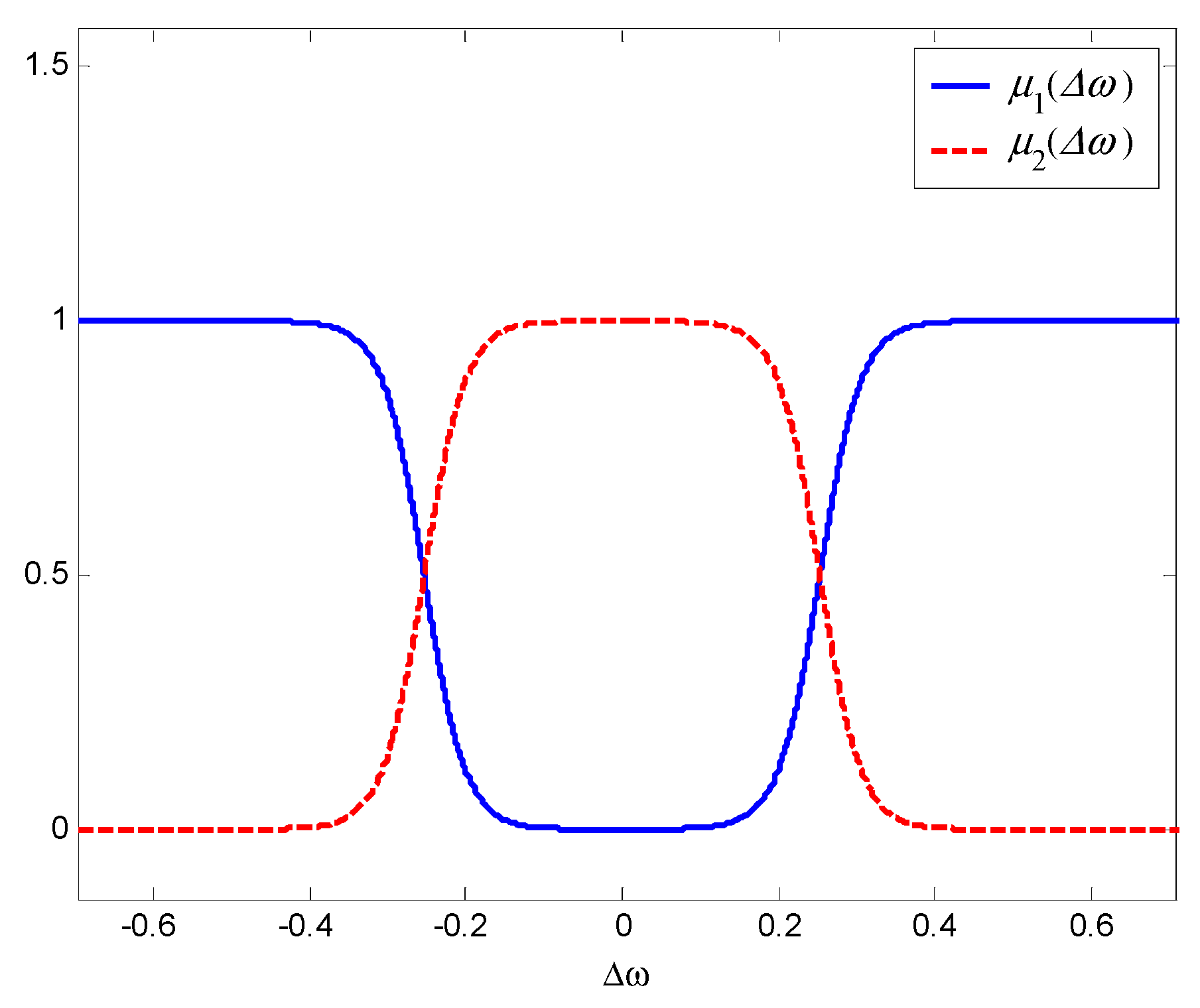
By choosing the membership functions

$${\mu }_1\left(\Delta \omega \right)=\frac{1}{1+e^{-38\left(\left|\Delta \omega \right|-0.253\right)}},{\mu }_2\left(\Delta \omega \right)=1-\frac{1}{1+e^{-38\left(\left|\Delta \omega \right|-0.253\right)}}$$

(48)

which represent the linguistic values LARGE and SMALL for the fuzzy variable $\Delta \omega$ (see Figure 5), the control input takes the following form:

$$E_f={\mu }_1\left(\Delta \omega \right)E_{f,NC}+{\mu }_2\left(\Delta \omega \right)E_{f,AVR/PSS}$$

(49)

This switching approach can also be utilized in the SVC compensator design. Specifically, a coordinated control strategy can be used in the SVC, which ensures that, initially, the power angle generator oscillations are rapidly damped, and then the SVC bus voltage is regulated towards its nominal value. To this end, a soft switching approach is adopted. The controllers switch when the large power angle deviations have been sufficiently mitigated so that the ancillary action of the SVC controller is no longer needed. The magnitude of the frequency deviation can serve as a switching criterion. In the new steady state, the SVC controller is transformed to a PI controller of the following form:

$$u_{B,V}\left(t\right)=k_P\Delta V_B\left(t\right)+k_I{\displaystyle {\int }_0^t\Delta V_B\left(\tau \right)d\tau }$$

(50)

and the combined control law is then

$$u_B\left(t\right)={\mu }_1\left(\Delta \omega \left(t-\tau \left(t\right)\right)\right)u_{B,NC}\left(t\right)+{\mu }_2\left(\Delta \omega \left(t-\tau \left(t\right)\right)\right)u_{B,V}$$

(51)

Obviously, the control law that employs delayed generator measurements can improve the transient stability only if the magnitude of the communication delays is small enough. After a careful examination of the simulation studies and taking into account the fact that the first peak in the oscillatory power angle response occurs at about 1 s after fault, a critical time of approximately 250 ms after fault can be defined. All measurements after a fault and up to this time can be used in the scheme we described above. Thus, the control law (51) should be modified to ensure that, for delays larger than 250 ms, a classical voltage PI is used, whereas, for delays smaller than or equal to 250 ms, the proposed nonlinear controller is used.

The following Takagi–Sugeno fuzzy rules implement the overall soft switching approach.

$$\begin{array}{l}{R}_1:\mathrm{IF}\left|\Delta \omega \left(t-\tau \left(t\right)\right)\right|\mathrm{is}\mathrm{LARGE}\mathrm{AND}\tau \left(t\right)\mathrm{is}\mathrm{SMALL}\mathrm{THEN}{u}_B\left(t\right)=u_{B,NC}\left(t\right)\\ R_2:\mathrm{IF}\left|\Delta \omega \left(t-\tau \left(t\right)\right)\right|\mathrm{is}\mathrm{SMALL}\mathrm{THEN}{u}_B\left(t\right)=u_{B,V}\left(t\right)\\ R_3:\mathrm{IF}\tau \left(t\right)\mathrm{is}\mathrm{LARGE}\mathrm{THEN}{u}_B\left(t\right)=u_{B,V}\left(t\right)\end{array}$$

The membership functions

$${\overline{\mu }}_1\left(\tau \left(t\right)\right)=\frac{1}{1+e^{-100\left(\tau \left(t\right)-0.25\right)}}$$

(52)

and

$${\overline{\mu }}_2\left(\tau \left(t\right)\right)=1-{\overline{\mu }}_1\left(\tau \left(t\right)\right)$$

(53)

are selected for the linguistic values LARGE and SMALL of the fuzzy variable $\tau \left(t\right)$. Thus, the SVC controller is given by

$$u_B\left(t\right)=\frac{{\mu }_1\left(\Delta \omega \left(t-\tau \left(t\right)\right)\right)\cdot {\overline{\mu }}_2\left(\tau \left(t\right)\right)\cdot u_{B,NC}\left(t\right)+\left[{\overline{\mu }}_1\left(\tau \left(t\right)\right)+{\mu }_2\left(\Delta \omega \left(t-\tau \left(t\right)\right)\right)\right]\cdot u_{B,V}}{{\mu }_1\left(\Delta \omega \left(t-\tau \left(t\right)\right)\right)\cdot {\overline{\mu }}_2\left(\tau \left(t\right)\right)+{\overline{\mu }}_1\left(\tau \left(t\right)\right)+{\mu }_2\left(\Delta \omega \left(t-\tau \left(t\right)\right)\right)}$$

(54)

It is obvious from the previous discussion that the magnitude of the communication delays is crucial. If these are large, then the proposed overall control scheme cannot provide the desired improvement as it will work only as a voltage controller. However, the latency times in current WLAN communication networks (3G, 4G) do not exceed 100 ms. They are even smaller in ADSL and VDSL Internet connections. Thus, both are viable options for communicating the distant measurements.

6. Simulation Studies

The simulation studies were performed in MATLAB/Simulink on an Intel Core i3-2348M PC at 2.30 GHz with 4 GB RAM. For our simulation scenario, the system parameters are adopted from [16], that is, $D=5.0$ p.u., $M=4.0$ s, $x_d=1.863$ p.u., $x_d^{\prime }=0.657$ p.u., $x_{T1}=x_{T2}=0.127$ p.u., $x_{L1}=x_{L2}=0.2426$ p.u., $T_{d0}^{\prime }=6.9$ s, ${\omega }_0=314.159$ rad/s, $B_{L0}=1$ p.u., $B_c=1$ p.u., $T_B=0.2$ s, and $\left|k_c{u}_f\right|\le 6$. The operating point considered is $\delta ={41.7}^{°}$, $P_e=0.8$ p.u., and $V_t=1.0$ p.u. The nonlinear excitation controller parameters are chosen as $c_1=4$, $c_2=4$, $c_3=50$, and the gain in the nonlinear SVC controller is taken as $c_B=5$. The AVR/PSS parameters are selected to be $K_a=21$, $T_a=0.05$, $T_1=0.3$, $T_2=0.1$, $T_r=0.4$, and $K_{PSS}=0.1$, and the gains of the PI voltage controller are chosen as $K_P=1$ and $K_I=10$.

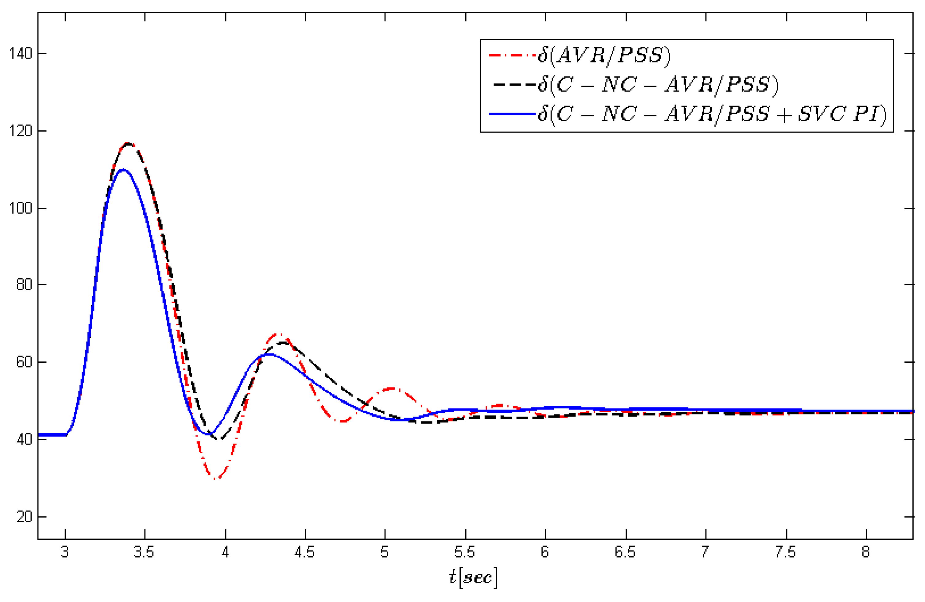
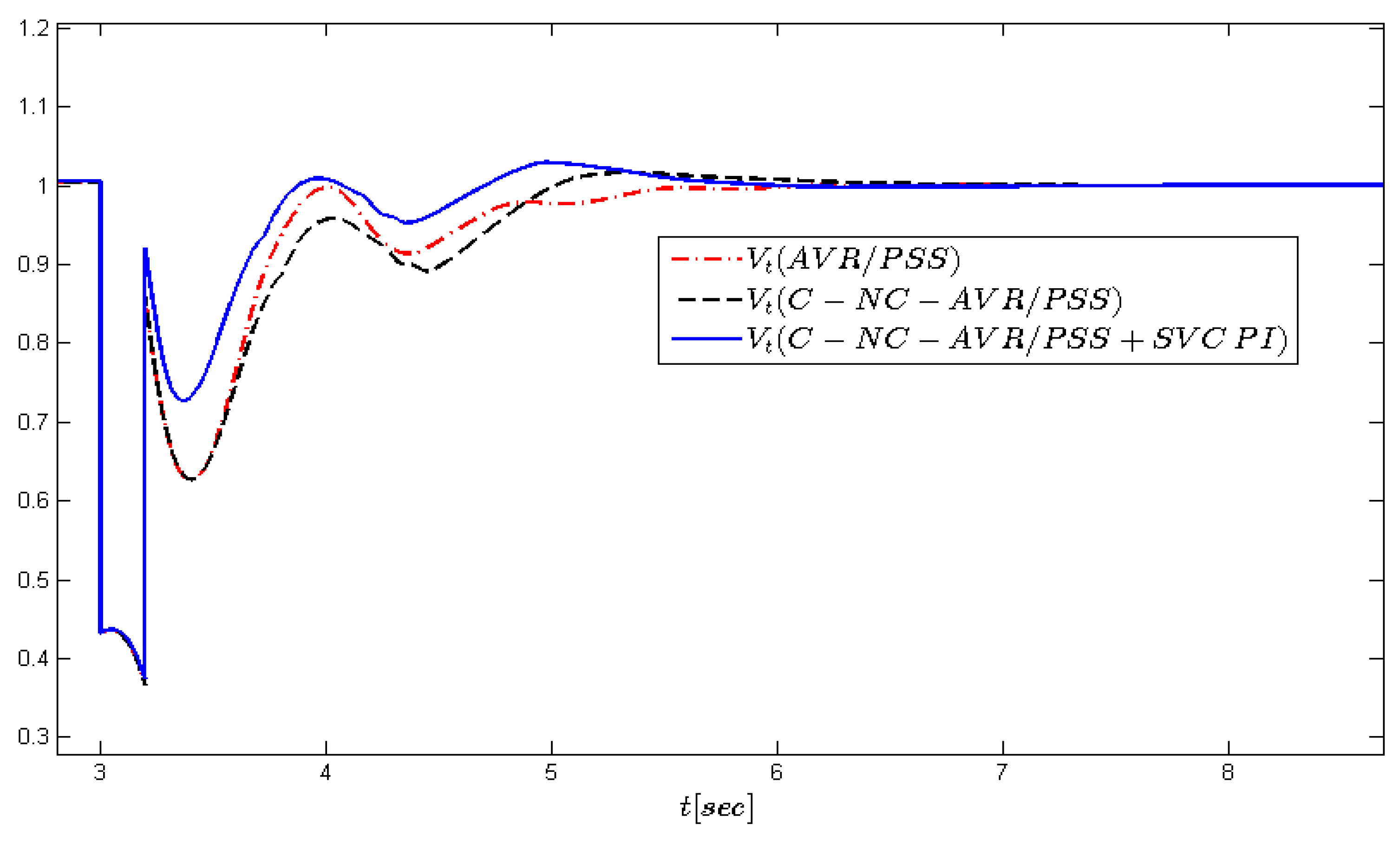
A symmetrical three-phase fault occurs at time $t=3\sec$ in the middle of one of the two lines connecting the generator and SVC buses ($k=0.5$). Breakers open after 200 ms and the line remains open. Both the power angle response (Figure 6) and the terminal voltage response (Figure 7) demonstrate the effectiveness of the SVC compensator in improving the transient stability of the power system. Comparisons are made between three different cases. In particular, the proposed coordinated nonlinear stabilizer with the AVR/PSS and PI SVC controller (case 1: C-NC-AVR/PSS+SVC PI) is compared with the coordinated nonlinear stabilizer with the AVR/PSS controller (case 2: C-NC-AVR/PSS) and the simple AVR/PSS (case 3) controller.

Figure 6 shows that the power angle oscillations after the simulated large fault are significantly reduced by the action of the proposed coordinated nonlinear stabilizer of case 1. For the other two, it is seen that the case 2 controller provides a better response than that of case 3. Figure 7 indicates the voltage response after the fault. The superiority of the proposed coordinated nonlinear stabilizer is apparent, while in all cases, the inclusion of the AVR/PSS controller effectively eliminates the steady-state deviation of the voltage amplitude.

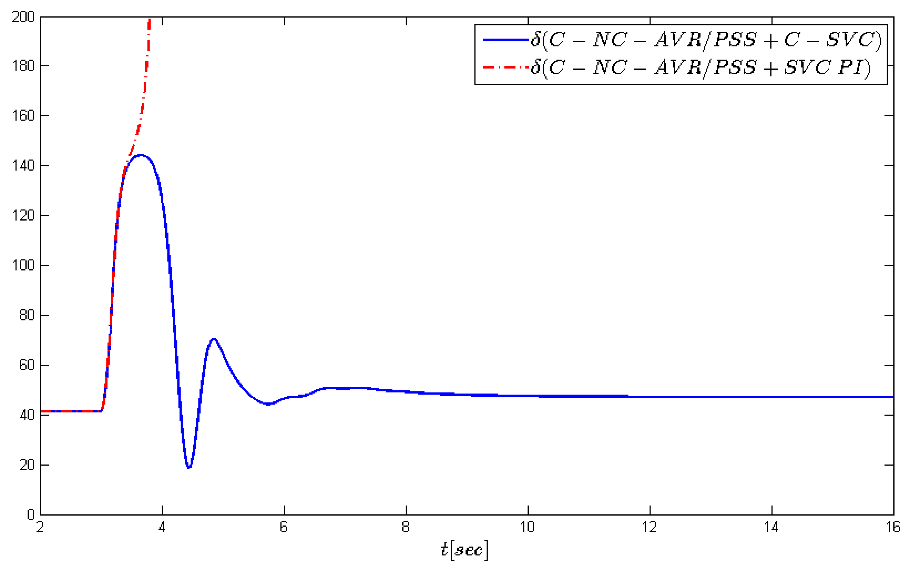
For the case of a more severe fault closer to the generator bus ($k=0.21$), which is again removed after 200 ms, we compare the two control schemes: the coordinated nonlinear stabilizer with AVR/PSS and PI SVC controller (C-NC-AVR/PSS+SVC PI) and the coordinated nonlinear stabilizer with AVR/PSS and coordinated SVC control (C-NC-AVR/PSS+C-SVC).

Even though the PI SVC controller can help in reducing the undesired oscillations after a fault, Figure 8 indicates that its action is not sufficient to avoid loss of synchronization for a fault that occurs so close to the generator. The C-NC-AVR/PSS+C-SVC controller on the other hand can efficiently return the system to the equilibrium point, avoiding loss of synchronism.

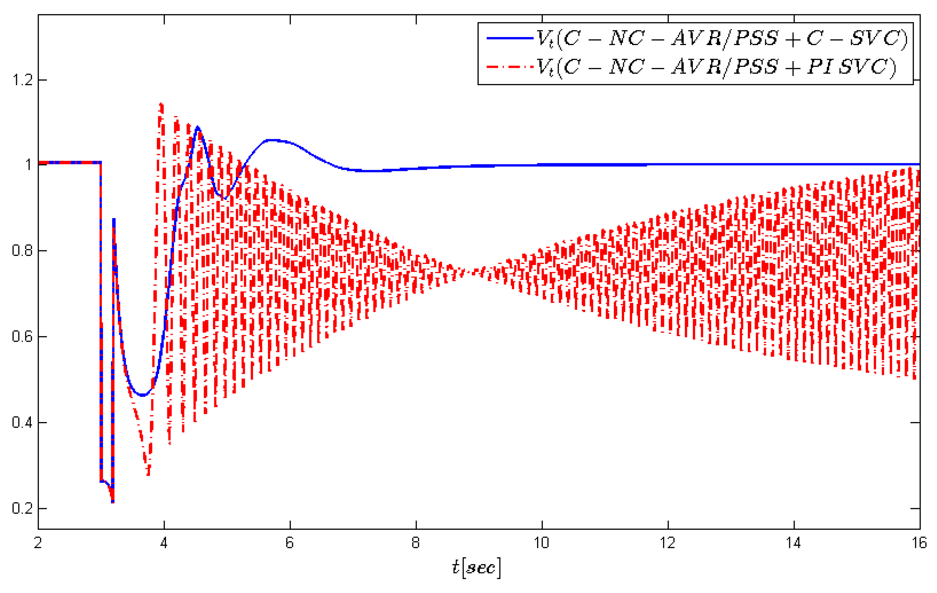
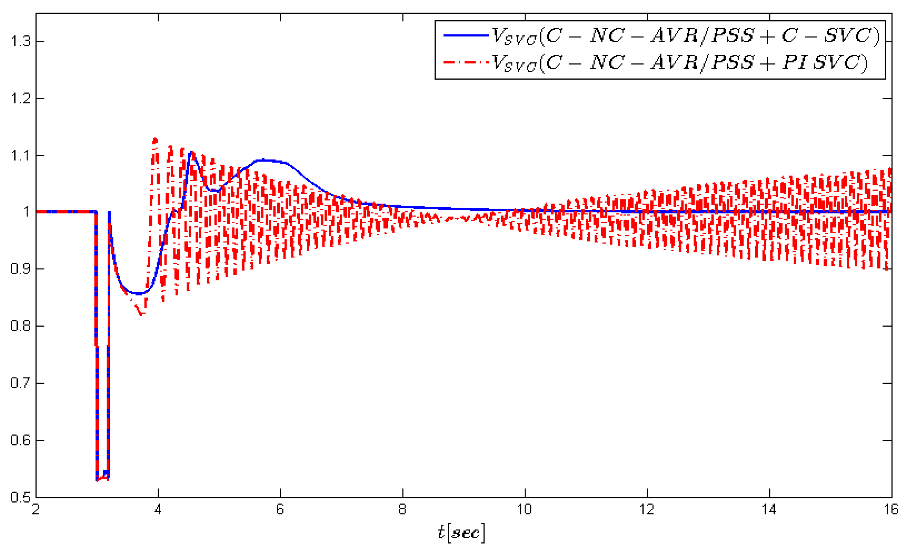
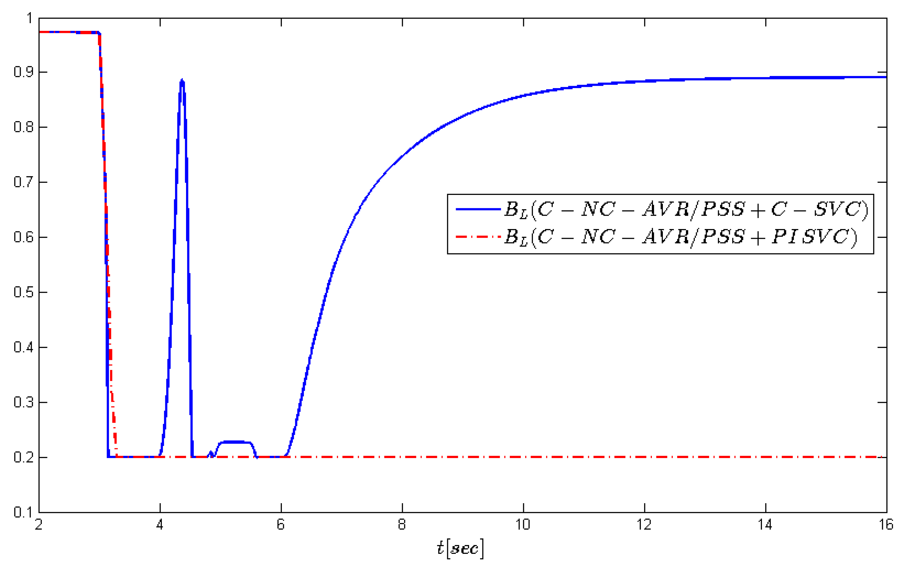
Figure 9, Figure 10 and Figure 11 show the generator terminal voltage response, the SVC bus voltage response, and the varying susceptance in the SVC compensator, respectively, under the proposed C-NC-AVR/PSS+C-SVC and C-NC-AVR/PSS+SVC PI controllers. Unstable oscillations for $V_t,V_{SVC}$ occur under the C-NC-AVR/PSS+SVC PI controller, whereas the C-NC-AVR/PSS+C-SVC controller can effectively regulate voltages at the generator and SVC bus to their nominal values.

7. Conclusions

A new coordinated excitation and SVC control is proposed for regulating the output voltage and improving the transient stability of a synchronous generator infinite bus (SGIB) power system. By regulating the SVC susceptance using distant from the generator, and thus delayed, measurements, the SVC can potentially improve the overall transient performance and stability. The time delays that further complicate the rigorous analysis conducted are taken into account and impose the limits and conditions that are adequate for the proposed controller to be efficient and stable. The scheme is completed by a soft-switching mechanism used to recover the output voltage level at the terminal bus and the SVC bus after the large power angle deviations have been eliminated.

References

1. Yu, Y.N. Electric Power System Dynamics; Academic Press: New York, NY, USA, 1983. [Google Scholar]
2. Alexandridis, A.T. Studying state convergence of input-to-state stable systems with applications to power system analysis. Energies 2020, 13, 92. [Google Scholar] [CrossRef] [Green Version]
3. Gao, L.; Chen, L.; Fan, Y.; Ma, H. A nonlinear control design for power systems. Automatica 1992, 28, 975–979. [Google Scholar] [CrossRef]
4. Roy, T.K.; Mahmud, M.A.; Shen, W.X.; Amanullah, M.T. An adaptive partial feedback linearizing control scheme: An application to a single machine infinite bus system. IEEE Trans. Circuits Syst. II Express Briefs 2019. (early access). [Google Scholar] [CrossRef]
5. Psillakis, H.E.; Alexandridis, A.T. A new excitation control for multimachine power systems I: Decentralized nonlinear adaptive control design and stability analysis. Int. J. Control Autom. Syst. 2005, 3, 278–287. [Google Scholar]
6. Shamsollahi, P.; Malik, O.P. Application of neural adaptive power system stabilizer in a multi-machine power system. IEEE Trans. Energy Convers. 1999, 14, 731–736. [Google Scholar] [CrossRef]
7. Psillakis, H.E.; Alexandridis, A.T. A simple nonlinear adaptive-fuzzy passivity-based control of power systems. Nonlinear Dyn. Syst. Theory 2007, 7, 51–67. [Google Scholar]
8. Psillakis, H.E.; Alexandridis, A.T. A new excitation control for multimachine power systems II: Robustness and disturbance attenuation analysis. Int. J. Control Autom. Syst. 2005, 3, 288–295. [Google Scholar]
9. Liu, Z.Q.; Yao, W.; Wen, J.Y. Enhancement of power system stability using a novel power system stabilizer with large critical gain. Energies 2017, 10, 449. [Google Scholar] [CrossRef]
10. Wang, H.F.; Swift, F.J. A unified model for the analysis of FACTS devices in damping power system oscillations. I. Single-machine infinite-bus power systems. IEEE Trans. Power Deliv. 1997, 12, 941–946. [Google Scholar] [CrossRef]
11. Kotsampopoulos, P.; Georgilakis, P.; Lagos, D.T.; Kleftakis, V.; Hatziargyriou, N. FACTS providing grid services: Applications and testing. Energies 2019, 12, 2554. [Google Scholar] [CrossRef] [Green Version]
12. Safa, A.; Sakhaeifar, M. Mismatched disturbance attenuation control for static var compensator with uncertain parameters. Int. J. Electr. Power Energy Syst. 2017, 91, 61–70. [Google Scholar] [CrossRef]
13. Shi, H.; Sun, X.; Chen, G.; Zhang, H.; Tang, Y.; Xu, L.; Xu, Y. Optimization Strategy of SVC for Eliminating Electromagnetic Oscillation in Weak Networking Power Systems. Energies 2019, 12, 3489. [Google Scholar] [CrossRef] [Green Version]
14. Wan, Y.; Murad, M.A.A.; Liu, M.; Milano, F. Voltage frequency control using SVC devices coupled with voltage dependent loads. IEEE Trans. Power Syst. 2018, 34, 1589–1597. [Google Scholar] [CrossRef]
15. Wang, Y.; Tan, Y.L.; Guo, G. Robust nonlinear coordinated generator excitation and SVC control for power systems. Int. J. Electr. Power Energy Syst. 2000, 22, 187–195. [Google Scholar] [CrossRef]
16. Cong, L.; Wang, Y.; Hill, D.J. Transient stability and voltage regulation enhancement via coordinated control of generator excitation and SVC. Int. J. Electr. Power Energy Syst. 2005, 27, 121–130. [Google Scholar] [CrossRef]
17. Wan, Y.; Zhao, J.; Dimirovski, G.M. Robust adaptive control for a single-machine infinite-bus power system with an SVC. Control Eng. Pract. 2014, 30, 132–139. [Google Scholar] [CrossRef]
18. Liu, Y.; Li, J.; Ding, Q.; Chu, B. Energy-based coordinated nonlinear control of synchronous generator and static var compensator. Int. J. Electr. Power Energy Syst. 2012, 43, 131–140. [Google Scholar] [CrossRef]
19. Zhang, X.; Wang, S.; Zhu, G.; Ma, J.; Li, X.; Chen, X. Decentralized robust adaptive neural dynamic surface control for multi-machine excitation systems with static var compensator. Int. J. Adapt. Control Signal Process. 2019, 33, 92–113. [Google Scholar] [CrossRef] [Green Version]
20. Li, J.; Chen, Z.; Cai, D.; Zhen, W.; Huang, Q. Delay-dependent stability control for power system with multiple time-delays. IEEE Trans. Power Syst. 2015, 31, 2316–2326. [Google Scholar] [CrossRef]
21. Milano, F.; Anghel, M. Impact of time delays on power system stability. IEEE Trans. Circuits Syst. I Regul. Pap. 2011, 59, 889–900. [Google Scholar] [CrossRef]
22. Guo, Y.; Hill, D.J.; Wang, Y. Global transient stability and voltage regulation for power systems. IEEE Trans. Power Syst. 2001, 16, 678–688. [Google Scholar] [CrossRef]
23. Anderson, P.M.; Fouad, A.A. Power System Control and Stability; The Iowa State University Press: Ames, IA, USA, 1977. [Google Scholar]
Figure 1. Simplified generator and static var compensator (SVC) three-bus model. AVR/PSS, automatic voltage regulator and power system stabilizer; TCR, thyristor controlled reactor; FC, fixed capacitor.
Energies 13 02181 g001
Figure 2. Pre-fault equivalent circuit.
Energies 13 02181 g002
Figure 3. Equivalent circuit during fault.
Energies 13 02181 g003
Figure 4. Post-fault equivalent circuit.
Energies 13 02181 g004
Figure 5. The membership functions.
Energies 13 02181 g005
Figure 6. Generator power angle responses (in degrees).
Energies 13 02181 g006
Figure 7. Generator terminal voltage response (in p.u.).
Energies 13 02181 g007
Figure 8. Power angle deviations (in degrees).
Energies 13 02181 g008
Figure 9. Generator terminal voltage responses (in p.u.).
Energies 13 02181 g009
Figure 10. SVC bus voltage responses (in p.u.).
Energies 13 02181 g010
Figure 11. The varying susceptances in the SVC compensator (in p.u.).
Energies 13 02181 g011