Optimization of Operating Parameters for Stable and High Operating Performance of a GDI Fuel Injector System

Abstract

In this study, a novel injector driving circuit was developed to achieve the regulation of fuel injection quantity and to work with the engine control system in a vehicle. The main purpose of the proposed injector driving circuit is to control the quantity and timing of fuel injection within the gasoline direct injection (GDI) fuel injector system. In this paper, a mathematical state model of a high-pressure (H.P.) fuel injector system is derived and the improved Taguchi method is proposed to define the optimal operating parameter settings of a fuel injector system. The experiments on fuel injection quantity were performed to achieve the requirements of the injector driving circuit. The fuel quantity sprayed from a fuel injector system under these control parameters was analyzed by leading the design of experiments. The S/N and β slopes were analyzed to determine their optimal control settings. The H.P. injector driving circuit developed was designed to drive the fuel injector and spray the injected quantity of fuel into the flask following the optimized control factors. The experimental results demonstrate that the H.P. fuel injecting system exhibits better and more stable operating performance, to assure the accurate injection quantity for the GDI injector, and it was also realized with low cost metal oxide semiconductor field effect transistor (MOSFET) switches.

1. Introduction

Gasoline direct injection (GDI) technology operates in a mode that directly injects fuel into the cylinder and ignites the fuel. A GDI fuel injecting system directly squirts fuel into the cylinder of the GDI engine. The high-pressure injector is the most important element in the engine, and it has gained significant attention and the interest of researchers on gasoline direct injection (GDI) engines, due to Euro 6 emission standards reducing emissions, and economic and efficiency concerns [1,2]. This mode of operation differs from traditional port fuel injection (PFI), thus avoiding a cold start. Since the cylinder temperature is not high enough to cause the fuel to vaporize instantaneously, resulting in difficulty to achieve ignition, the ECU usually injects more fuel, even more than the equivalent quantity of fuel burned. Therefore, GDI technology has been a superior option for improving fuel economy and emission reductions. The article has been examined for the effect of ambient temperature on the formation of fuel adhesion, and the mechanisms behind it [3]. This study enhances knowledge of the spray–wall interactions under various engine-like conditions. In the paper, the wall-impinging spray performance is explored based on its microscopic characteristics [4]. This review paper [5,6] provides a comprehensive survey on recent progress and findings in PM number reduction techniques and PM number emissions research on GDI engines. The study of direct injection gasoline engines has become a focus of research concerning the development of a high-performance injector driving circuit in recent years due to its high thermal efficiency, lower fuel consumption, and better cold start performance. The fuel economy and superior performance for GDI engines are of significant importance to other engine researchers who will perform similar experiments and investigations. These surveys have been done to review and discuss all of the available GDI literature in detail [7]. The injector driving circuit projected in a coupled simulation model of injector electromagnetic and needle rigid body motion has has been attempted to optimize the setting values of two-stage current waveforms [8]. The optimal current strategy was determined for driving the fuel injector under different fuel supply pressures. Three stage currents with two stage on-time duties, and final stage PWM operation were obtained based on the magnetic force requirement to achieve a better operating performance of the driving circuits [9]. A high-pressure GDI injector drive was developed to implement the fuel injection quantity for a 500cc motorbike engine. The control parameters of the programmable injector drive circuit can be optimized by a preset current profile [10]. The injector drive circuit was illustrated and the operating parameters were optimized by controlling the current flowing through the solenoid injector coils. This significantly quickens the response time of the control valve [11,12,13]. An experimental result shows that the current drive circuit is a feasible and reliable option to use for practical injector application in the GDI engines. It worked successfully and efficiently and was compatible with the high-pressure (H.P.) injector. The PWM operation was applied to measure the fuel injection quantities of the H.P. injector defined as the fuel injection curves by tuning the control parameters of the injector drive circuit [14]. The flow characteristics of a pump injector have been investigated and carried out in simulations and experiments by using different driving circuits. A self-designed logic control circuit was proposed to achieve peak and hold current control without software intervention [15,16]. Taguchi method adopts a set of orthogonal arrays, which promotes a minimum number of experiments and provides maximum information about all control factors affecting the results [17]. There are numerous studies using the Taguchi method in engine testing applications. The Taguchi method for obtaining optimal combination of those parameters was discussed in [18,19,20].

A superior H.P. injector driving circuit introduced into engines that are modified to inject gasoline directly into the combustion chamber was developed by using the Taguchi method in the optimization of the H.P. fuel injecting system. One of the most important developments for GDI engines is the H.P. fuel injecting system. The injector driving circuit is designed to satisfy the fast high-pressure injector response for sustaining the instantaneous surge voltages and currents. Therefore, power transistors in the H.P. injector driving circuit were replaced by power metal oxide semiconductor field effect transistors (MOSFETs) because of their superior performance and rapid response. The H.P. injector driving circuit was made into a printed circuit board (PCB) board to examine the dynamic performance of the H.P. injector. A three stage driving current was implemented by adjusting pulse durations and PWM operation added to the last pulse duration.

The GDI fuel injector system has been modeled and examined on a laboratory prototype test platform to validate the performance. To demonstrate the operation capability, a laboratory prototype was fabricated and tested under various dynamic operating parameters. In the following section, the system principles and operations are introduced. The system modeling is followed by the H.P. injector driving circuit description. Section 3 gives a description of the experimental setup. Section 4 illustrates a dynamic response of the GDI fuel injector system and comparative analysis of proposed control operating parameters with the Taguchi method. The present work proposes a systematic procedure and statistical methodology of Taguchi robust optimization design L8 orthogonal array (OA) for evaluating the best factor-level with its application on the case studies of optimization problems for fuel injection quantity.

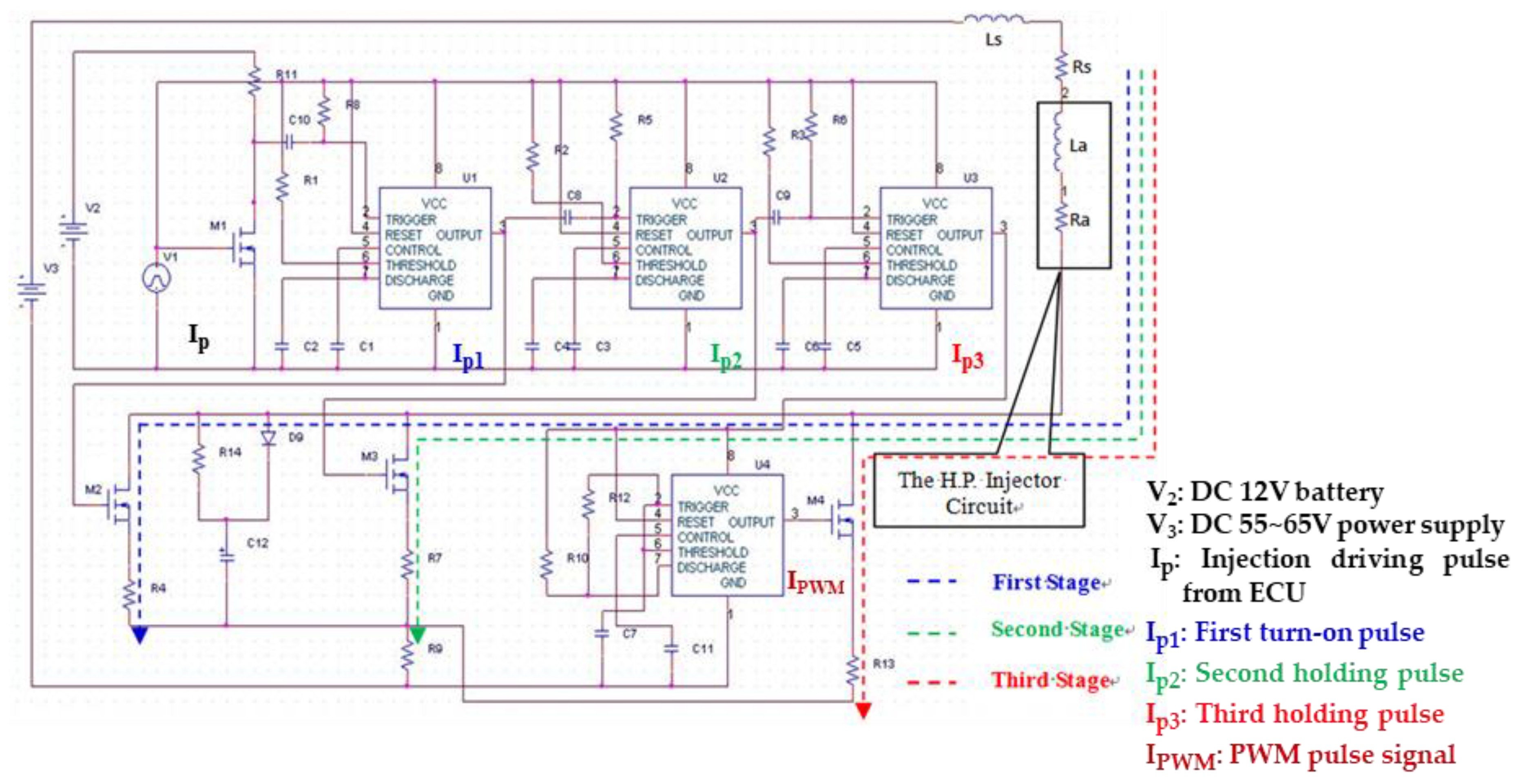
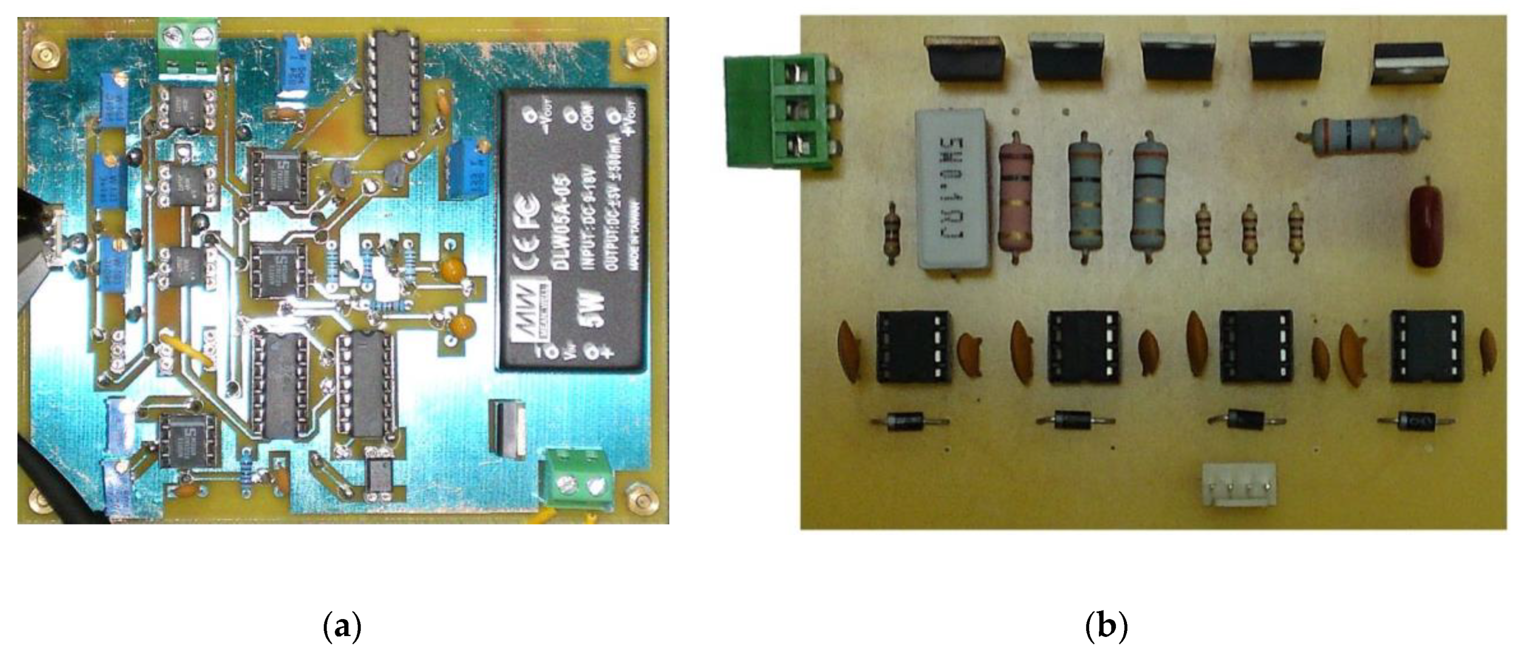
2. Design of the H.P. Injector Driving Circuit

The influence of fuel supply pressure, engine speed, first-stage turn-on injector driving current, second-stage injector holding current, and power supply voltages on fuel injection quantity is investigated in the paper. The results showed that the injection quantity corresponding to the same injection pulse width increases gradually with the increase of injection pressure. Pspice simulation software was applied to implement on simulation of the injector driving circuit for the requirements of the GDI injector characteristics. The simulation was based on common requirements for automotive applications. The PSpice model of the three-stage power MOSFETs injector driving circuit with driver ICs is illustrated in Figure 1. Consequently, a ready-made circuit model was acquired, which can be analyzed and redesigned at a later stage. Three-stage power MOSFETs were introduced in the design of the injector driving circuit to carry on the experiments under the operations of high-frequency surge voltages and currents. After the simulations and experiments with PWM operation were added into the last pulse duration, the improved injector driving circuit was required to be made into PCB boards. Two circuit boards were made and then the components were soldered into the PCB boards, as shown in Figure 2a,b. The experimental results measured by the PCB boards were compared with those as shown in the simulation. This not only saved modeling time, but also reduced the time and amount of data in the simulation stage and analysis of results.

2.1. Principle and Operation

In this study, a gasoline direct injection (GDI) measurement system mainly including a Bosch H.P. single-hole injector was tested, along with the fuel supply system and its driver with a control circuit. A data acquisition system was implemented on the injection pulse width duration, fuel injection quantity, and fuel injection pressure. In order to improve the opening response performance of the injector in the cylinder of the direct injection engine, high and low voltage drive circuits were developed for the injector. An electrical driving circuit with three pulse width and PWM controller was applied to the H.P. GDI injector. It consisted of a CPD-100-030PR programmable power supply module (DC 0–100 V, 30 A), automotive battery DC 12 V, three sets of NE555 timer IC U1-U3, a PWM control IC U4, three opt isolator 4N35 ICs for signal processing, and four high-side power N-Channel MOSFETs. A current sensing resistor and an H.P. injector represented an in-series R_L circuit. Three driving pulse signals were inputted to drive the power MOSFETs switches of the injector driving circuit via the opt isolator driving IC 4N35, of which the functions were dealt with the signal processing and anti-noise performance. An engine control unit (ECU) outputs trigger signals of 5 V DC, being unable to turn the MOSFET switches on. The trigger signals were required from DC 5V to boost up to at least voltage level DC 12 V by a boost converter to drive the MOSFET switches M2–M4. It actually has adjusted the time or shape of the signal sequence, as shown in the Figure 3a,b depending on the pulse duration of an engine control unit (ECU). Figure 1 shows typical pulse waveforms with three different durations controlled by R₁, R₈ and C₁₀; R₂, R₅ and C₈; R₃, R₆ and C₉ connected to U₁, U₂, and U₃ respectively. The PWM modulation circuit is U₄ illustrated in Figure 1. The PWM profiles were generated during PWM operation. The high-level duration t_H and low-level duration t_L of NE555 outputs U₁, U₂, and U₃ can be calculated as t_H = 0.693(R₁₀ + R₁₂)C; t_L = 0.693(R₁₂)C [10].

Other useful equations are given as follows: Period = t_H + t_L = 0.693(R₁₀ + 2R₁₂)C. The switching frequency curves of PWM operation are shown as the red line of Figure 9c in the paper [10]. The IC U3 output pulse signal was input into the IC U4 to obtain the PWM control signal. Three-stage power MOSFETs were introduced into the design of the injector driving circuit. The adjustable pulse duration of an engine control unit (ECU) is equal to the pick-up stage I (200 μs) + holding stage I (400 μs) + the last pulse PWM duration (Stage III is adjustable.) The H.P. injector coils are activated under three-pulse-width (12/5/3A) peak and holding current profiles to produce the electromagnetic force to withdraw and hold the needle of the injector, therefore ensuring superior injector performance.

2.2. Modeling and Characterization

The three-stage power MOSFETs injector driving circuit can be employed in driving a high-pressure solenoid injector actuator. A power MOSFETs injector driving circuit which directly controls the charging/discharging current by power MOSFETs is simple. Based on the working principles of three-stage power MOSFETs injector driving circuits, a circuit was designed as a programmable driving module. It consisted of a boost converter, a first-stage charging MOSFET M2, a second-stage charging MOSFET M3, a third-stage PWM charging MOSFET M4, a current sensing resistor, and an injector solenoid (in-series inductor). A freewheeling diode placed across the inductive load in the driving circuit will provide a path for the release of energy stored in the inductor while the load voltage drops to zero. Depending on the ON/OFF states of the different MOSFETs, current flow routes are different. A state equation based 2nd RLC electric circuit model described as (1) is implemented for the development of the high-pressure solenoid injector driving module.

$$\{\begin{array}{l}{L}_T\frac{di}{dt}+(R_T+R_4+R_9)i=V_0\hspace{1em}0\le t\le t_{FS}\hfill \\ L_T\frac{di}{dt}+(R_T+R_7+R_9)i=V_0\hspace{1em}{t}_{FS}\le t\le t_{SS}\hfill \\ L_T\frac{di}{dt}+(R_T+R_{13}+R_9)i=V_0\hspace{1em}{t}_{SS}\le t\le t_{TS}\hfill \\ L_T\frac{di}{dt}+(R_T+R_{14}+R_9)i+\frac{1}{C_p}{\displaystyle \int i}dt=V_0\hspace{1em}{t}_{TS}\le t\le t_{DC}\hfill \end{array}$$

(1)

where L_s/L_a are the input and actuator inductances, L_T = L_s + L_a; i is the actuator current; R_s/R_a are the input and actuator resistances, R_T= R_s + R_a; R₄/R₇/R₉/R₁₃/R₁₄ are the resistances to limit the peak pick-up current; V_o is the initial voltage across the actuator, V_c and C_p—the charge voltage and capacitance of capacitor. T_FS/T_SS/T_TS are the time periods of the first stage, second stage, and third stage charging current profile respectively. T_DC is the time period of discharging current. For high-pressure solenoid actuated injectors, the working voltage applied on the solenoid actuator is decisive for the fuel injection quality, due to the actuator displacement. Injection stability is assured by achieving working supply voltage. The executing voltage is required to reduce overshoot or oscillation. When the charging current is not properly controlled, the overshoot and oscillation may occur into the injector supply voltage. The injector driving circuit is usually a series RLC circuit and under-damped due to its low resistance. Optimum driving current profile can be described in Figure 3a. Therefore, control of the charging/discharging current profile is very important for the design of an H.P. injector driving module. Also, different injectors are needed to redesign their inductance value. In the injector driving circuit applications, current modulation by controlling the MOSFET using pulse width modulation (PWM) is commonly adopted. The series inductor is for the purpose of providing smooth current and available energy storage. Generally, the selected inductance value is 100–220 μH in the applications of the injector. The fast last stage PWM operation period is around an interval of 600–1200 μs for a solenoid injector driver, as described in Figure 3b.

3. Experimental Configuration and Equipment

The fuel injection quantity of the injector directly affects the formation, combustion, and emissions of the mixture in the cylinder of the direct injection gasoline engine. The fuel injection system testing the fuel injection characteristics was established to carry out the internal relationship between the fuel injection process and the combustion process in the cylinder of the GDI engine. A novel injector driving circuit was made to provide for the in-cylinder direct injection gasoline engine, and discussed in the paper. In this paper, a fuel injection experiment for the H.P. fuel injection system was studied to develop a stable and accurate injector drive circuit. Experimental results were analyzed to provide the best injection factor for an H.P. fuel injector drive circuit. The H.P. fuel injection quantity was tested by the fuel injector driving circuit at DC 55–65 V power supply voltage, 80–100 bar fuel pressure, and 1200–2000 μs fuel injection pulse duration. Next, the Taguchi method was used to determine the optimal parameter settings for the H.P. fuel injector drive circuit. Four important control factors, namely the power supply voltage, the first turn-on injector drive current, the second injector holding current, and the fuel supply pressure. The effect of the M-y response of the H.P. on the injector has been explored to determine the optimal control factors for its injector drive circuit. Finally, the Taguchi method for establishing the optimal factor set is discussed. The confirmation experiments for the original and new designs were reviewed for the H.P. injector performance.

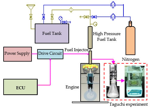
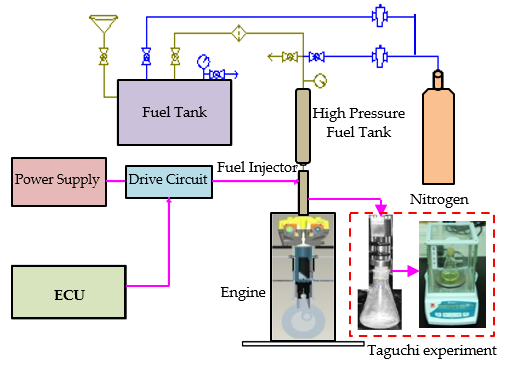
3.1. High-Pressure Fuel Supply System

The H.P. fuel injector used in this study was a single-hole atomizing injector with solenoid valve swirling gasoline, which is produced by BOSCH. Its plunger is opened inward and the product ID is BOSCH 026150026. The hole diameter of the injector and degree of decentralization are 549 micrometers and 12 degree respectively. The fuel injector has an operating pressure of 80–100 bar and is now commonly applied in GDI engines. In order to reduce the negative effects of the high-pressure fuel pump operation on the H.P. injector in the cylinder of GDI engines, a high-pressure fuel supply system was used, which forced the high-pressure nitrogen into the seamless stainless steel cylinder, and boosted the fuel injection pressure to the operating pressure 80–100 bar using the nitrogen pressure regulation valve. In the fuel supply system, the stainless fuel cylinder was pressurized the operating pressure up to 80–100 bar (max) by using the H.P. Nitrogen bottle, as illustrated in Figure 4. The MASS 2100 flow sensor was combined with the SITRANS F C MASS 6000 transmitters to make a complete flow meter for the experimental applications. The experimental instruments for characterizing the dynamic performances of the H.P. GDI injector are illustrated in Figure 5a,b. After characterizing the dynamic performance of the injector, as shown in Figure 6, the fuel pressure in the GDI Bosch injector installed on the cylinder head of a 500cc motorcycle engine was set to 80–100 bar in the experiment.

3.2. General Operating Principle

In-cylinder direct injection technology has potential fuel economy and emission reductions advantages. It is a superior option choice in that a GDI fuel injection system which a high-pressure injector is the central component. A high-pressure fuel supply system of GDI engines directly injects fuel to the cylinder of the engine. The time and duration of fuel injection are electronically controlled by the ECU. The ECU sends TTL pulse signals to the injector driver as an input to the system to trigger the driver charging the actuator from 55 V to 65 V. A variety of pulse durations are sent to the fuel injector driving circuit in accordance with the actual operating conditions from the signal of the engine sensor. The high-pressure fuel injection system mainly includes four parts: the fuel supply system; the ECU; the electric drive circuit; and the injector. The fuel system supplies a constant 80–100 bar pressure resource for the injector. Timing diagram of the pulse duration control are controlled by using an ECU that calculates and analyzes analog and digital input signals from various engine sensors. Engine performance can be improved by more rapid engine response in the throttle positions and more accurate control of air-fuel ratio. In this study, a Bosch GDI single-hole injector was installed and measured on 500cc cylinder heads of a motorcycle engine.

3.3. Mathematical Model

The H.P. fuel injector system consists of three main coupled components: (1) the fuel flow part; (2) the solenoid coil and driver; and (3) the needle lift of injectors. These subsystem models can be given by the following nonlinear state equations of a fuel injection system. The solenoid coil and driver model will be indicated by the states ${\overrightarrow{\mathrm{X}}}_1$ = [B $\dot{B}$]^T , the fuel injection model by the states ${\overrightarrow{\mathrm{X}}}_2$ = [P_bv], and the needle lift of injectors by $\overrightarrow{\mathrm{X}}$₃ =[x $\dot{x}$ P_uv P_lv u $\dot{u}$ z $\dot{z}$ y $\dot{y}$]^T. α₁ , α₂ , α₃ , β₁ , β₂ , and β₃ are given functions of inputs and states to define model outputs or state derivatives [16].

Solenoid coil driver model:

$$\stackrel{°}{\overrightarrow{\mathrm{x}}}{}_2={\overrightarrow{\mathsf{\alpha }}}_1({\overrightarrow{\mathrm{x}}}_1,{\overrightarrow{\mathrm{u}}}_1)=\overrightarrow{{\mathsf{\alpha }}_1}\left(\left[\begin{array}{c}B\\ \dot{B}\end{array}\right], \left[\begin{array}{c}{V}_{in}\\ u\end{array}\right]\right)$$

(2)

$${\overrightarrow{\mathrm{y}}}_1=\left[\begin{array}{c}{V}_s\\ B\end{array}\right]={\overrightarrow{\beta }}_1 ({\overrightarrow{\mathrm{x}}}_1,{\overrightarrow{\mathrm{u}}}_1)={\overrightarrow{\beta }}_1\left(\left[\begin{array}{c}B\\ \dot{B}\end{array}\right], \left[\begin{array}{c}{V}_{in}\\ u\end{array}\right]\right)$$

(3)

Fuel flow model:

$$\stackrel{°}{\overrightarrow{\mathrm{x}}}{}_2={\overrightarrow{\mathsf{\alpha }}}_2({\overrightarrow{\mathrm{x}}}_2,{\overrightarrow{\mathrm{u}}}_2)=\overrightarrow{{\alpha }_2}\left(\left[P_{bv}\right], \left[\begin{array}{c}{P}_{cyl}\\ x\\ P_{tank}\\ P_{uv}\end{array}\right]\right)$$

(4)

$$\stackrel{°}{\overrightarrow{\mathrm{y}}}{}_2=\left[\begin{array}{c}{P}_{vb}\\ {\omega }_{iof}\end{array}\right]={\overrightarrow{\beta }}_2 ({\overrightarrow{\mathrm{x}}}_2,{\overrightarrow{\mathrm{u}}}_2)=\overrightarrow{{\beta }_2}\left(\left[P_{bv}\right], \left[\begin{array}{c}{P}_{cyl}\\ x\\ P_{tank}\\ P_{uv}\end{array}\right]\right)$$

(5)

Needle lift system model:

$$\stackrel{°}{\overrightarrow{\mathrm{x}}}{}_3={\overrightarrow{\mathsf{\alpha }}}_3({\overrightarrow{\mathrm{x}}}_3,{\overrightarrow{\mathrm{u}}}_3)=\overrightarrow{{\alpha }_3}\left(\left[\begin{array}{c}x\\ \dot{x}\\ P_{uv}\\ P_{lv}\\ \begin{array}{c}u\\ \dot{u}\\ \begin{array}{c}z\\ \dot{z}\end{array}\\ y\\ \dot{y}\end{array}\end{array}\right], \left[\begin{array}{c}{P}_{bv}\\ B\\ P{L}_{s1}\\ P{L}_{s2}\\ P{L}_{s3}\\ P{L}_{tot}\end{array}\right]\right)$$

(6)

$$\mathrm{c}\overrightarrow{\mathrm{y}}{}_3=\left[\begin{array}{c}x\\ P_{uv}\\ u\end{array}\right]={\overrightarrow{\beta }}_3 ({\overrightarrow{\mathrm{x}}}_3,{\overrightarrow{\mathrm{u}}}_3)=\overrightarrow{{\beta }_3}\left(\left[\begin{array}{c}x\\ \dot{x}\\ P_{uv}\\ P_{lv}\\ \begin{array}{c}u\\ \dot{u}\\ \begin{array}{c}z\\ \dot{z}\end{array}\\ y\\ \dot{y}\end{array}\end{array}\right], \left[\begin{array}{c}{P}_{bv}\\ B\\ P{L}_{s1}\\ P{L}_{s2}\\ P{L}_{s3}\\ P{L}_{tot}\end{array}\right]\right)$$

(7)

where PL_s1, PL_s2, PL_s3, and PL_tot are the preloads for the upper volume spring of the needle, return spring of the needle, lower volume spring of the needle, and all injector springs respectively. The complete states of the subsystem models are P_bv, P_lv, P_uv, x, $\dot{\mathrm{x}}$ , u, $\dot{\mathrm{u}}$ , z, $\dot{\mathrm{z}}$, y, $\dot{\mathrm{y}}$, B, and $\dot{B}$.

4. Experimental Design and Data Analysis

This paper proposes a novel injector drive circuit to measure the fuel injection quantity sprayed into an Erlenmeyer flask from the injector by using the Taguchi method. The fuel injection quantity was analyzed under different control factors, such as fuel supply pressure, engine speed, supply voltages, and injector currents. A fluid Erlenmeyer flask was used to receive the fuel quantity sprayed out from the injector and then weighed and recorded by the precise electronic balance. The Taguchi method was designed to measure the fuel injection quantity. Its fuel injection time can be changed by the pulse signal generator to vary its fuel injection quantity with corresponding engine speed. The Taguchi measurement was used as an experimental basis on which signal-to-noise (S/N) ratios and β slopes were analyzed to determine its optimal control level, and the flowchart for optimization of controlled operating factors of a high-pressure injector is shown in Figure 7.

4.1. Equations of β, Sd, and S/N Ratios

Experiments were measured for N1 and N2 in the morning and the afternoon respectively. There were 20 sampling data points for each Taguchi experiment to calculate β value. The β value is the slope of the regression line for the 20 raw data points, and can be indicated as [17]:

$$\beta =\frac{{\displaystyle \sum _{i=1}^n{M}_i{y}_i}}{{\displaystyle \sum _{i=1}^n{M}_i^2}}$$

(8)

Standard deviation is a measure of the variation or discreteness in statistics set of data points. A low standard deviation shows that the value tends to be close to the expected value of the data set, whereas a high standard deviation indicates that the value is distributed over a wide range. The standard deviation may be abbreviated as S_d. The sample standard deviation can refer to one of the above amount as applied to those data when only samples of experimental data from the population are available. The S_d value expresses the deviation error of the regression line from the sampling data point, which was calculated as follows [17]:

$$S_d=\sqrt{\frac{{\displaystyle \sum _{i=1}^n{(y_i-\beta M_i)}^2}}{n-1}}$$

(9)

The basic idea of the Taguchi method was executed to select several control factors using an orthogonal table to perform a systematic experiment, measure the quality characteristics, and calculate the signal-to-noise (S/N) ratio. The above data was employed to establish an empirical formula to describe the relationship between S/N ratio and control factors. Using this experimental mode, we can easily know which control factor combination can maximize the S/N ratio. The S/N ratio response is given by the following equation [17]:

$$\mathsf{\eta }\mathrm{dB}=S/N=-10\log \frac{S\frac{2}{d}}{{\beta }^2}$$

(10)

If the quality characteristics have a certain target, we can classify the control factors, some are used to maximize the S/N ratio, and some are used to adjust the quality characteristics to align with the target. Greater values of the S/N ratio determine control factor settings that minimize the effects of the noise factors. The experimental mode was constructed under certain assumptions, and usually requires more experiments to confirm the accuracy of this experimental mode.

4.2. The First Taguchi Experiment

The pulse widths and numbers are set by pulse-delayed generator. Experiments were measured for N1 and N2 in the morning and the afternoon respectively. Each experiment was performed twice—the first measurement was named Q1 and the second measurement named Q2 for confirming the precision of the fuel injection measurement system. The operating factors were set as supply voltage, injector current, engine speed, and fuel supply pressure (as shown in

Table 1. Control factors for fuel injection quantities and corresponding levels (first Taguchi measurement).

Labels	Control Factor	Units	Level 1	Level 2	Level 3
A	Supply voltage	V	55	60	65
B	First stage current	A	8	10	12
C	Speed	RPM	2400	6000	9000
D	Fuel supply pressure	bar	80	90	100

), to optimize the design and measurement of the fuel injection quantity in the experiment. The parameter settings were chosen without affecting the variances. D level was represented as the fuel supply pressure. The level of factor D fuel supply pressure contributed the highest percentage, but the variances were too large. The best control factor level with small percentage and high contribution was the A and B level for controlling the supply voltage and first stage injector current. S/N ratio response, β slope, and ANOVA analysis were employed to assess the experimental results, as illustrated in

Table 2. Raw data of β Slope and S/N ratio for the L9 orthogonal array of dynamic control factors for the H.P. injector.

L9	M = 1200 μs				M = 1400 μs				M = 1600 μs				M = 1800 μs				M = 2000 μs				β	Sd	S/N
	N1		N2		N1		N2		N1		N2		N1		N2		N1		N2
	Q1	Q2	Q1	Q2	Q1	Q2	Q1	Q2	Q1	Q2	Q1	Q2	Q1	Q2	Q1	Q2	Q1	Q2	Q1	Q2
1	11.331	11.265	11.401	11.367	13.124	13.211	13.121	13.087	15.119	15.398	15.243	15.133	17.149	16.943	17.043	17.198	19.079	19.178	19.086	18.984	9.490	0.117	38.197
2	12.266	12.305	11.253	12.278	14.029	14.993	14.095	14.084	16.398	16.432	16.289	16.341	18.397	18.345	18.434	18.376	20.600	20.498	20.675	20.532	10.219	0.298	30.703
3	15.398	15.302	15.407	15.374	14.617	14.598	14.681	14.677	16.637	16.703	16.749	16.598	18.938	18.821	19.078	18.987	20.963	21.078	20.898	20.877	10.731	1.185	19.141
4	12.635	12.643	12.598	12.698	14.690	14.672	14.735	14.683	16.935	17.103	16.943	16.881	19.305	19.434	19.406	19.287	21.411	21.501	21.478	21.378	10.653	0.168	36.048
5	11.594	11.601	11.577	11.612	13.439	13.407	13.486	13.507	15.896	15.843	15.971	15.799	17.755	17.687	17.854	17.789	19.808	19.764	19.854	19.932	9.836	0.202	33.734
6	12.234	12.246	12.308	12.209	14.363	14.384	14.401	14.334	16.307	16.391	16.402	16.251	18.541	18.398	18.601	18.579	20.526	20.411	20.576	20.654	10.257	0.083	41.880
7	11.912	11.983	11.871	11.923	13.849	13.879	13.911	13.861	15.888	15.838	15.909	15.793	18.040	18.165	17.986	18.109	20.001	20.134	20.165	20.012	9.984	0.114	38.871
8	12.904	12.891	11.032	12.911	14.885	14.906	14.867	14.919	17.111	17.071	17.045	16.972	19.445	19.395	19.502	19.487	21.549	21.689	21.601	21.587	10.704	0.429	27.937
9	11.746	11.735	11.762	11.741	13.795	13.832	13.763	13.781	15.638	15.731	15.593	15.691	17.761	17.846	17.702	17.802	19.655	19.743	19.632	19.753	9.838	0.070	43.001

. This Taguchi experiment helped to most economically study significance of four factors on the required quality characteristic. By considering the effect of individual factors on the fuel injection quantity, the optimum combination of factors could be obtained.

The computed formulas for S/N noise ratio and β value are represented for factor response analysis. The larger the slope of the noise factor, the better the characteristics. The best level of the S/N noise ratio was taken as A2, B1, C2, and D1, as shown in Figure 8a,b.

The F value and the percentage of contribution were selected without affecting the number of variations. The ANOVA results showed that level D contributed the highest percentage, but the quantity of variation was too large, because the characteristics of the high pressure injector and the manufacturer's recommended value were driven. The upper limit of voltage and current, therefore was chosen as A2-B1-C2-D1 with a small percentage of variation and high contribution. The levels of factors A and B were utilized to control the injector voltage and current, and level D as the fuel pressure level (as shown in

Table 3. ANOVA analysis (first Taguchi measurement).

Labels	Variance	Freedom	Sum of Squares	F	Contribution
A	0.5	2	0.2	0.03	2.72%
B	6.1	2	3.1	0.34	28.64%
C	0.6	2	0.3	0.04	3.53%
D	77.6	2	38.8	4.35	97.13%

).

The S/N noise ratios and β slopes can be repeated to achieve the required injection quality under the optimized operating conditions. The prediction analysis of the original and new designs (as shown in

Table 4. Predicted values of signal-to-noise (S/N) ratio and β for the original and new designs (first Taguchi measurement).

Factor	Original Design			New Design
		Response			Response
	Setting	S/N	β	Setting	S/N	β
A	1	29.1	10.147	2	37.0	10.249
B	1	37.5	10.042	1	37.5	10.150
C	1	35.8	10.150	2	36.4	10.236
D	1	38.1	9.721	1	38.1	9.721
Average		34.2	10.190		34.2	10.190
Predicted value		38.0	9.490		46.4	9.786

) was performed and then raw data, β Slope, and S/N ratio for the original and new designs (as shown in

Table 5. Raw data, β Slope and S/N ratio for the original and new designs (first Taguchi measurement).

Exp					M = 1200 μs				M = 1400 μs				M = 1600 μs				M = 1800 μs				M = 2000 μs				β	S	S/N
					N1		N2		N1		N2		N1		N2		N1		N2		N1		N2
	A	B	C	D	Q1	Q2	Q1	Q2	Q1	Q2	Q1	Q2	Q1	Q2	Q1	Q2	Q1	Q2	Q1	Q2	Q1	Q2	Q1	Q2
Original	1	1	1	1	11.775	11.792	11.732	11.727	13.409	13.416	13.354	13.342	15.321	15.303	15.278	15.287	17.037	17.028	17.007	17.005	18.933	18.927	18.923	18.911	9.530	0.175	34.713
New	2	1	3	1	12.739	12.638	12.691	12.813	14.925	14.876	15.012	14.957	17.036	17.102	16.998	17.086	18.972	18.987	19.051	19.093	21.509	21.598	21.481	21.551	10.666	0.138	37.779

) were performed. It can be observed from the M-y graph in that the fuel injection point of the original design deviates from the straight line, which causes an error in the injector fuel injection quantity, as shown in Figure 9a. The fuel injection point of the new design was very close to a straight line, as shown in Figure 9b. The error caused by the new design does not deviate much from the predicted value due to the change in level. Therefore, the optimized fuel injection factors were closer to the ideal fuel injection test value.

4.3. Confirmation Experiments

In order to improve the M-y diagram as shown in the first Taguchi experiment, the second experiment was performed to reach the deviation point set between 1200 μs and 1800 μs so that it approached a linear fit. The second Taguchi experiment was realized at different supply voltage (V), current (A), second stage holding current (A), fuel supply pressure (bar), and pulse width time in the designed table. The Taguchi control factors were set to supply voltage, first stage turn-on current, and second stage injector current, and the fuel supply pressure was optimized for second measurement of fuel injection quantity, as shown in

Table 6. Control factors for fuel injection quantities and corresponding levels (second Taguchi measurement).

Labels	Factor	Units	Level 1	Level 2	Level 3
A	Supply voltage	V	55	60	65
B	First-stage turn-on current	A	8	10	12
C	Second-stage holding current	A	*3	*4	*5
			4	5	6
D	Fuel pressure	bar	80	90	100

* Enhancing second-stage holding current (3/4/5)A into (4/5/6)A

. The second experiment was achieved by having the second stage holding current instead of the speed (RPM) in the first experimental data. The S/N variances were observed and the optimization test was performed as shown in

Table 7. Second experiments for the original and new designs.

Exp					M = 1200 μs				M =1400 μs				M = 1600 μs				M = 1800 μs				M = 2000 μs				β	S	S/N
					N1		N2		N1		N2		N1		N2		N1		N2		N1		N2
	A	B	C	D	Q1	Q2	Q1	Q2	Q1	Q2	Q1	Q2	Q1	Q2	Q1	Q2	Q1	Q2	Q1	Q2	Q1	Q2	Q1	Q2
Original	1	1	1	1	11.693	11.713	11.643	11.674	13.272	13.288	13.038	13.131	15.280	15.295	15.166	15.236	16.991	16.959	16.993	17.018	18.965	18.975	18.954	18.988	9.499	0.156	35.680
New	3	1	1	3	6.901	7.009	7.753	7.749	7.229	7.396	7.898	7.784	7.402	7.718	7.205	7.386	7.307	7.779	7.522	7.722	7.744	8.037	7.693	7.997	4.598	1.204	11.642

.

An excessive error of the S/N noise ratio occurred in the significance test for ANOVA for the first measurement in comparison with second measurement under the optimal operating conditions. In the Taguchi measurement, the predicted best S/N ratio and β level values were selected to perform the experimental confirmation under A3-B1-C1-D3. A major mutation compared with the first experiment was the insufficient fuel injection quantity in the experiment. The results in a previous paper showed that the needle of the high-pressure injector sometimes cannot continuously and effectively be held, resulting in insufficient injection quantity and engine misfire from many engine tests [21]. The novelty and contribution of this present draft is some improvements and discussions of this problem. Finally, the new conclusions were drawn and were obviously different from the previous studies. The high-pressure fuel injection system may be established, however, further research methodologies are required to be applied to the custom-made GDI injectors in the GDI engines. The methodology and results by improved Taguchi method can provide some useful suggestions for other designers and researchers, who will conduct investigations on analyzing and improving the performance of GDI control systems. The proposed experimental study of the characteristics of high-pressure GDI injectors is the main contribution of this article, which and can help researchers achieve superior performance in the case of GDI injectors with bounded errors due to control factors. Therefore, an experimental investigation using an improved Taguchi method on the characterization of a high pressure GDI injector is important for the required practical applications. It was found that the turn-on time of first stage voltage and current for the fuel injector were too short (only 180 μs). Also, the lower settings for second stage holding currents (3/4/5A) cannot continuously and effectively hold the needle of the high-pressure injector, resulting in insufficient injection quantity (see Table 7). Thus, the settings of first stage turn-on time and second stage holding currents were enhanced by 200 μs and 4/5/6A respectively for the third confirmation experiment.

Our confirmation experiment attempted to execute and statistically evaluate the fuel injection quantity with optimal control factors. The injection quality of the H.P. injector can be determined by the β slope and S/N ratio under optimal operating conditions. Control factors with different levels were performed to identify the optimized injection parameters and reach the optimal injection quality characteristics. The noise ratio and β slope can be repeated under the optimized operating conditions to determine the required injection quality. Prediction analysis was performed for the original and new designs, and then the measured values were acquired in the third experiment, as shown in

Table 8. Raw data, β Slope and S/N ratio for the L9 orthogonal array of dynamic control factors for the H.P. injector (third Taguchi measurement).

	M = 1200 μs				M = 1400 μs				M = 1600 μs				M = 1800 μs				M = 2000 μs				β	Sd	S/N
L	N1		N2		N1		N2		N1		N2		N1		N2		N1		N2
	Q1	Q2	Q1	Q2	Q1	Q2	Q1	Q2	Q1	Q2	Q1	Q2	Q1	Q2	Q1	Q2	Q1	Q2	Q1	Q2
1	11.693	11.713	11.643	11.674	13.272	13.288	13.038	13.131	15.280	15.295	15.166	15.236	16.991	16.959	16.993	17.018	18.965	18.975	18.954	18.988	9.499	0.160	35.457
2	12.841	12.854	12.849	12.864	14.478	14.503	14.543	14.558	16.596	16.629	16.612	16.631	18.394	18.428	18.504	18.535	20.479	20.527	20.545	20.564	10.351	0.231	33.040
3	13.205	13.284	13.268	13.358	15.083	15.118	15.177	15.197	17.014	17.025	17.228	17.274	19.023	19.045	19.297	19.348	21.128	21.151	21.414	21.456	10.731	0.246	32.780
4	12.729	12.778	12.793	12.806	14.521	14.540	14.579	14.644	16.763	16.789	16.825	16.863	18.679	18.695	18.832	18.851	20.915	20.934	20.992	21.037	10.480	0.126	38.421
5	12.306	12.286	12.358	12.339	13.876	13.904	14.060	14.061	15.905	15.947	15.966	16.002	17.683	17.716	17.812	17.842	19.627	19.681	19.719	19.743	9.942	0.219	33.122
6	12.651	12.675	12.747	12.773	14.534	14.579	14.649	14.678	16.486	16.536	15.592	16.638	18.506	18.536	18.685	18.733	20.439	20.493	20.617	20.657	10.335	0.282	31.270
7	12.419	12.428	12.385	12.402	14.169	14.179	14.176	14.182	16.295	16.323	16.263	16.288	18.174	18.187	18.175	18.178	20.206	20.253	20.253	20.309	10.154	0.120	38.555
8	13.016	13.043	13.045	13.067	14.783	14.834	14.895	14.916	17.092	17.128	17.118	17.155	19.096	19.145	19.168	19.235	21.282	21.327	21.325	21.383	10.682	0.125	38.652
9	12.462	12.438	12.442	12.446	14.237	14.254	14.269	14.294	16.158	16.196	16.203	16.229	18.007	18.024	18.067	18.090	19.894	19.932	19.939	19.965	10.089	0.212	33.541

. In the original and new designs, the fuel injection point of the original design deviates from a straight line, which causes an error in the fuel injection quantity (as shown in Figure 10a,b, in which the fuel injection point of the new design is very close to the straight line).

Table 9. ANOVA analysis (third Taguchi measurement).

Factor	SS	DOF	Var	F	Confidence	Significant?
A	19.4	2	9.7	2.997	83.98%	Yes
B	33.7	2	16.8	5.211	92.31%	Yes
C	Pooled					No
D	Pooled					No
Error	12.9	4	3.2	S =1.8
Total	66.0	8	8.2	*At least 80% confidence level

displays the significance test of the ANOVA in the third measurement under the set operating conditions. The third confirmation experiments and predicted values of the S/N ratio and β for the original and new designs were compared in

Table 10. Predicted values of S/N ratio and β for the original and new designs. (third Taguchi measurement).

Factor	Original Design			New Design
	Setting	Response		Setting	Response
		S/N	β		S/N	β
A	1	32.6	10.205	3	36.0	10.185
B	1	37.3	10.002	1	37.3	10.002
C	1	34.9	10.170	1	34.9	10.170
D	1	33.7	9.808	3	36.2	10.633
Mean value		34.6	10.218		34.6	10.218
Predicted value		34.7	9.530		40.5	10.334

and

Table 11. Confirmation experiments for the original and new designs.

Exp					M = 1200 μs				M = 1400 μs				M = 1600 μs				M = 1800 μs				M = 2000 μs				β	S	S/N
					N1		N2		N1		N2		N1		N2		N1		N2		N1		N2
	A	B	C	D	Q1	Q2	Q1	Q2	Q1	Q2	Q1	Q2	Q1	Q2	Q1	Q2	Q1	Q2	Q1	Q2	Q1	Q2	Q1	Q2
Original	1	1	1	1	11.775	11.792	11.732	11.727	13.409	13.416	13.354	13.342	15.321	15.303	15.278	15.287	17.037	17.028	17.007	17.005	18.933	18.927	18.923	18.911	9.530	0.175	34.713
New	3	1	1	3	12.581	12.578	12.521	12.527	14.348	14.352	14.307	14.322	16.537	16.551	16.514	16.515	18.491	18.502	18.476	18.481	20.616	20.618	20.614	20.609	10.309	0.103	40.021
	3	1	3	3	12.754	12.747	12.724	12.735	14.569	14.584	14.609	14.598	16.649	16.653	16.685	16.686	18.724	18.713	18.767	18.757	20.727	20.724	20.791	20.783	10.426	0.117	39.031

. It can be observed in the third experiment results that the original design control factors caused the deviation of fuel injection quantity from the linear injection curves. The new control factors drove the H.P. injector to squirt the approximate fuel injection quantity to the linear injection curves. The confirmation experiments present less deviation from the predicted values due to the levels of factor C being different. The H.P. injector operated with the optimized injection control factor spurts at the optimal fuel injection quantity.

The original and new designs were taken with the settings of A3-B1-C1-D3 and A3-B1-C3-D3 to implement the confirmation experiments. It was observed that variances between two experimental settings presented statistically insignificant differences for the fuel injection quantity. Therefore, the best level A3-B1-C1-D3 was used to obtain the M-y graphs, as shown in Figure 11a,b. The original and new M-y graphs were compared with the fuel injection factors in the third experiment. The fuel injection quantity of the new design had the steeper rising slope of straight line. Also, the distribution points of fuel quantity for both original and new designs were concentrated at the deviation range of the straight lines. The optimal fuel injection quantity between new and original designs was improved by 5.308 dB, as shown in

Table 12. Improvement dB value for the original and new designs.

	Level	Calculated	Predicted	Difference	Improvement
		S/N	S/N		dB
Original	A1B1BC1D1	34.713	34.965	−0.253	5.308
Optimal	A3B1BC1D3	40.021	36.651	3.371

.

5. Conclusions

The stability of an injector driving circuit was examined for the injection accuracy of an injector, carefully recording each correction of fuel injection quantity to carry out functional testing step by step. In this study, the improved Taguchi method was used in the design of high-pressure injector driving circuit for accomplishing the control factors in the experimental measurement to determine the optimization of operating parameters. The results predicted based on the Taguchi method were confirmed through experiments. Its circuit design provided a simple and rugged driving solution to improve the H.P. injector driving circuit as having stable and high operating performance to assure the accurate fuel injection quantity. Some conclusions from experimental results have been drawn as follows:

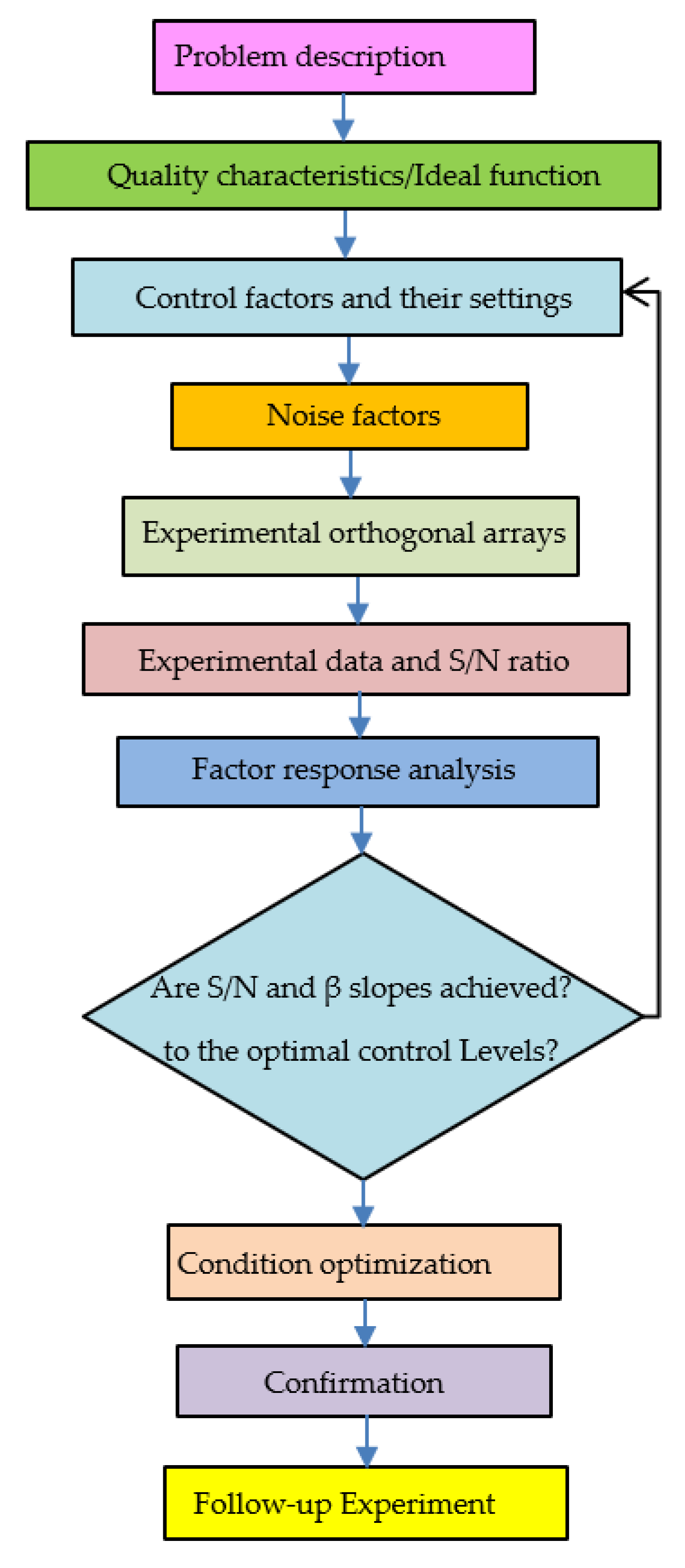
• This paper uses the orthogonal design experiment method, which can effectively list the percentage distribution of the results of all possible experiments, and then calculate the S/N ratios and β slopes of fuel injection quantity to determine the optimal injection factor levels. The significance of each control factor was confirmed by analysis of variation and optimal results were obtained.
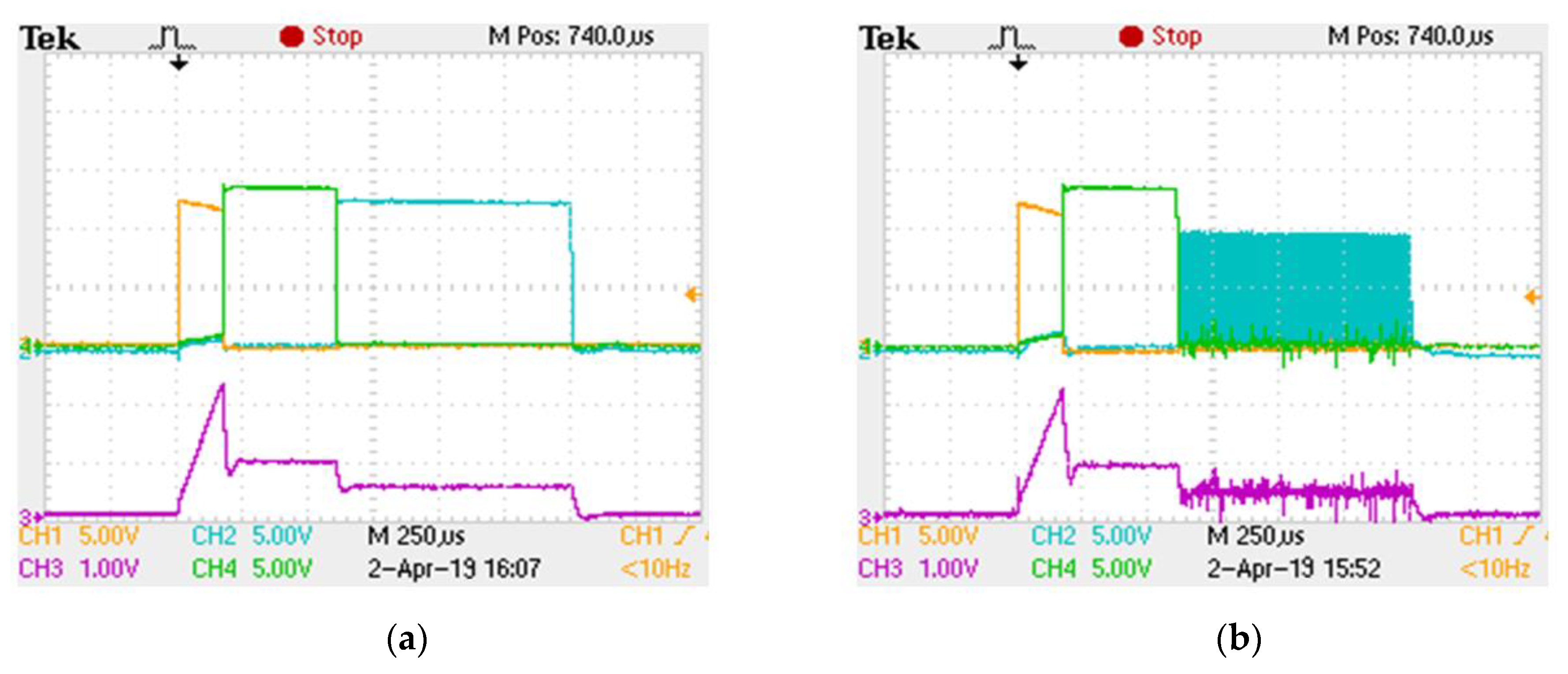
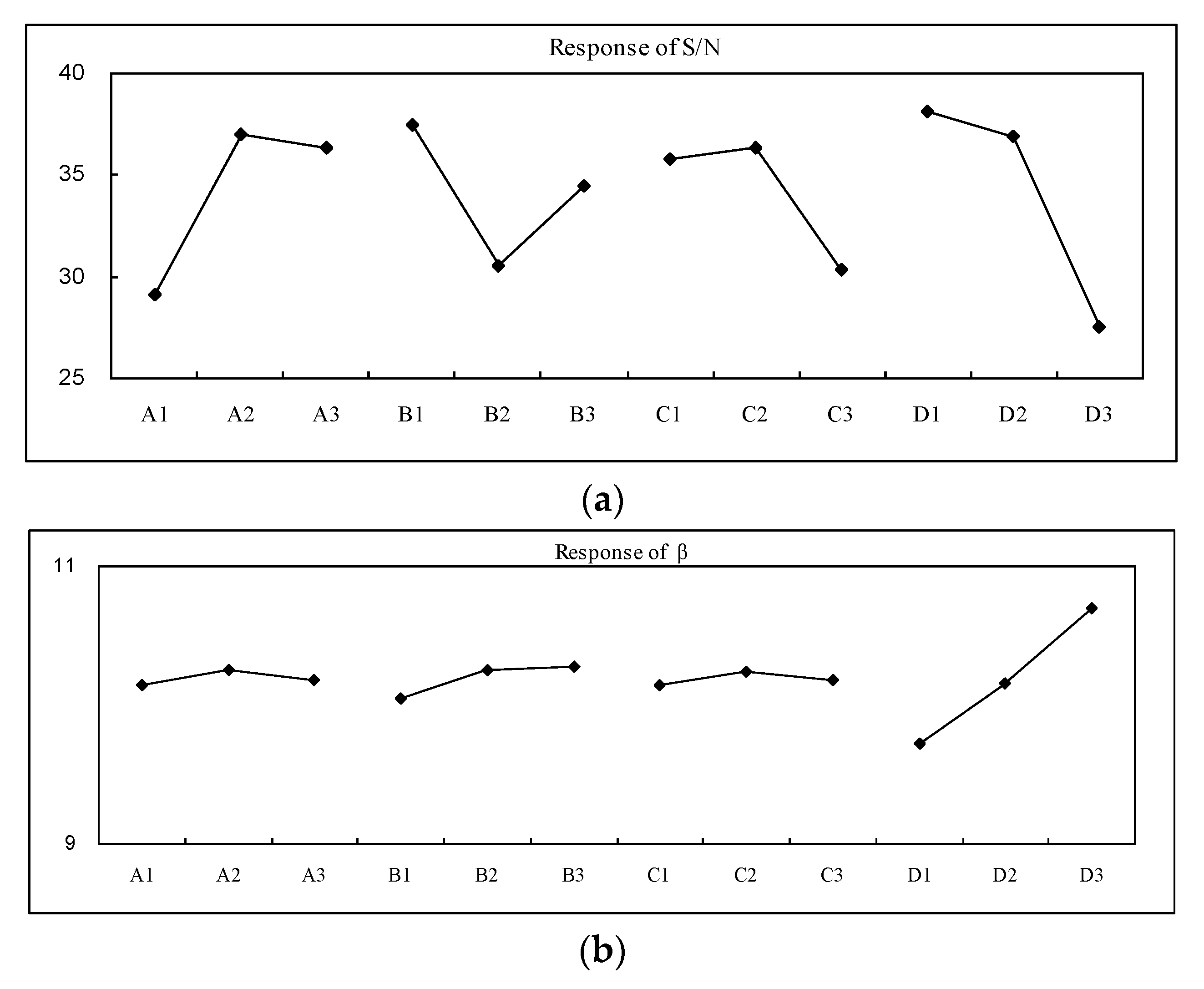
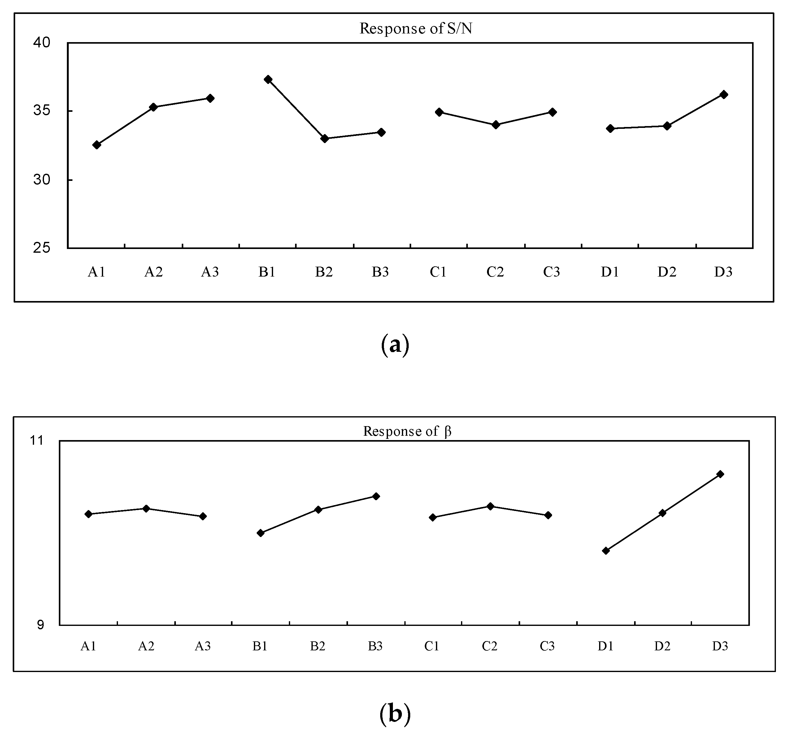
• It was found that the turn-on time of first stage injector current was too short (only 180 μs). The smaller settings of second stage holding currents (3/4/5A) could not continuously and effectively hold the needle of the high-pressure injector, resulting in insufficient injection quantity (see Table 7). Thus, the settings of the second stage holding currents were enhanced as (200 μs and 4/5/6A) for the third confirmation experiment.
• The Taguchi method is simple and feasible for testing and optimizing the design of high-pressure fuel injector drivers. It is also very effective in saving unnecessary testing time in experiments. The factor category that affects fuel injection quantity can be obtained from the cross-comparison of S/N ratios and β slopes using variation analysis. Factors A and B have the highest contribution. The optimal settings for supply voltage, the first stage turn-on, and second stage holding currents of an injector were determined to reduce the range of variation.
• The fuel supply pressure (factor D) was achieved to determine the maximum sensitivity by comparing the S/N ratios and β slopes, and therefore to significantly affect the fuel injection quantity. In Section 2.2, the original waveform of the injector driving current designed by BOSCH was adopted and improved. As a design consideration, the second-stage injector holding current (factor C) was used to reduce the cost.

Therefore, the experimental investigation in this paper is important in achieving the robust control required for practical application of this technology.

References

1. Zhao, F.; Lai, M.C.; Harrington, D.L. Automotive spark-ignited direct-injection gasoline engines. Prog. Energy Combust. Sci. 1999, 25, 437–562. [Google Scholar] [CrossRef]
2. Wang, C.; Xu, H.; Herreros, J.M.; Wang, J.; Cracknell, R. Impact of fuel and injection system on particle emissions from a GDI engine. Appl. Energy 2014, 132, 178–191. [Google Scholar] [CrossRef] [Green Version]
3. Luo, H.; Nishida, K.; Uchitomi, S.; Ogata, Y.; Zhang, W.; Fujikawa, T. Effect of temperature on fuel adhesion under spray-wall impingement condition. Fuel 2018, 234, 56–65. [Google Scholar] [CrossRef]
4. Luo, H.; Nishida, K.; Uchitomi, S.; Ogata, Y.; Zhang, W.; Fujikawa, T. Microscopic behavior of spray droplets under flat-wall impinging condition. Fuel 2018, 219, 467–476. [Google Scholar] [CrossRef]
5. Leach, F.; Knorsch, T.; Laidig, C.; Wiese, W. A Review of the Requirements for Injection Systems and the Effects of Fuel Quality on Particulate Emissions from GDI Engines; SAE Technical Paper; SAE International: Warrendale, PA, USA, 2018. [Google Scholar]
6. Raza, M.; Chen, L.; Leach, F.; Ding, S. A review of particulate number (PN) emissions from gasoline direct injection (GDI) engines and their control techniques. Energies 2018, 11, 1417. [Google Scholar] [CrossRef] [Green Version]
7. Jiangjian, A.; Xiyan, B.G.; Chunde, C.Y. An Experimental Study on Fuel Injection System and Emission of a Small GDI Engine. In Proceedings of the 2nd IEEE/ASME International Conference on Mechatronic and Embedded Systems and Applications, Beijing, China, 13–16 August 2006; pp. 1–6. [Google Scholar]
8. Zhang, X.; Palazzolo, A.; Kweon, C.B.; Thomas, E.; Tucker, R.; Kascak, A. Direct fuel injector power drive system optimization. SAE Int. J. Engines 2014, 7, 1137–1154. [Google Scholar] [CrossRef]
9. Tsai, W.C.; Yu, P.C.; Chen, K.H.; Guo, C.J. Development and Calibration of PC_Based Control System to Improve the Performance and Emissions of a 500cc Motorcycle Engine. ICIC Express Lett. 2010, 4, 2219–2226. [Google Scholar]
10. Tsai, W.C.; Yu, P.C. Design of the electrical drive for the high-pressure GDI injector in a 500cc motorbike engine. Int. J. Eng. Ind. 2011, 2, 70–83. [Google Scholar]
11. Huang, D.; Ding, H.; Wang, Z.; Huang, R. Design of drive circuit for GDI injector. In Proceedings of the 2011 International Conference on Electric Information and Control Engineering (ICEICE), Wuhan, China, 15–17 April 2011; pp. 5821–5824. [Google Scholar]
12. Qiang, C.; Zhang, Z.; Xie, N. Power losses and dynamic response analysis of ultra-high speed solenoid injector within different driven strategies. Appl. Therm. Eng. 2015, 91, 611–621. [Google Scholar]
13. Lu, H.; Deng, J.; Hu, Z.; Wu, Z.; Li, L. Impact of control methods on dynamic characteristic of high speed solenoid injectors. SAE Int. J. Engines 2014, 7, 1155–1164. [Google Scholar] [CrossRef]
14. Tsai, W.-C.; Zhan, T.-S. An Experimental Characterization for Injection Quantity of a High-pressure Injector in GDI Engines. J. Low Power Electron. Appl. 2018, 8, 36. [Google Scholar] [CrossRef] [Green Version]
15. Ji, H.; Wei, M.; Liu, R.; and Chang, C. Drive Control Simulation and Experimental Studies on the Flow Characteristics of a Pump Injector. IEEE Access 2020, 8, 35672–35681. [Google Scholar] [CrossRef]
16. Satkoski, C.; Shaver, G. Piezoelectric fuel injection: Pulse-to-pulse coupling and flow rate estimation. 568 IEEE-ASME T Mech. 2011, 16, 627–642. [Google Scholar] [CrossRef]
17. Lochner, R.H.; Matar, J.E. Designing for Quality. An Introduction to the Best of Taguchi and Western Methods of Statistical Method Design; Chapman & Hall: London, UK, 1990. [Google Scholar]
18. Ross, P.J. Taguchi Techniques for Quality Engineering, 2nd ed.; McGraw-Hill Inc.: New York, NY, USA, 1996. [Google Scholar]
19. Hedayat, A.S.; Sloane, N.J.A.; Stufken, J. Orthogonal Arrays: Theory and Applications; Springer: New York, NY, USA, 1999. [Google Scholar]
20. Lee, H.-H. Taguchi Methods: Principles and Practices of Quality Design; Gau Lih Book Co. Ltd.: Taipei, Taiwan, 2010. [Google Scholar]
21. Tsai, W.C.; Wu, Z.H. Use of Taguchi Method to Optimize the Operating Parameters of a High-Pressure Injector Driving Circuit. Appl. Mech. Mater. 2011, 130–134, 2795–2799. [Google Scholar] [CrossRef]
Figure 1. Electrical driving circuit diagram with three pulse width and pulse width modulation (PWM) operation added to the last pulse duration.
Energies 13 02405 g001
Figure 2. The Power metal oxide semiconductor field effect transistors (MOSFETs) driving circuit board with three-pulse control signals. (a) Logic operation and driving signal circuit board, (b) Three-pulse MOSFET driving circuit board.
Energies 13 02405 g002
Figure 3. (a) The driving pulse signals and gasoline direct injection (GDI) injector current profiles without PWM switching operation added to the last pulse duration (Ip1 = 180 μs), (b) The driving pulse signals and GDI injector current profiles with PWM switching operation added to the last pulse duration (Ip1 = 180 μs).
Energies 13 02405 g003
Figure 4. The high-pressure (H.P.) fuel supply and injecting system (Static measurement; 80–100 bar Max).
Energies 13 02405 g004
Figure 5. Dynamic Injection quantity measurements of the H.P. injector. (a) SITRANS F C MASS 2100 sensor, (b) MASS 6000 transmitter.
Energies 13 02405 g005
Figure 6. The GDI engine test stand with the H.P. fuel supply and injecting system (80–100 bar Max)
Energies 13 02405 g006
Figure 7. Flow chart for optimization of operating factors of a high-pressure fuel injection system.
Energies 13 02405 g007
Figure 8. (a) S/N ratio response graph (first Taguchi measurement), (b) β slope response graph (first Taguchi measurement).
Energies 13 02405 g008
Figure 9. (a) Original design M-y graph (first Taguchi measurement), (b) newly design M-y graph (first Taguchi measurement).
Energies 13 02405 g009
Figure 10. (a) S/N ratio response graph (third Taguchi measurement), (b) β slope response graph (Third Taguchi measurement).
Energies 13 02405 g010
Figure 11. (a) Original design M-y graph (third measurement), (b) new design M-y graph (third measurement).
Energies 13 02405 g011