Abstract
Energy-saving and energy-recovery strategies represent key factors to achieve operational cost reductions within rail systems’ management tasks. However, in altering service features, they also affect passenger satisfaction. This paper investigates the effect of implementing such measures in the case of rolling stock unavailability. Numerous operational scenarios were explored by analysing different planned headway and rolling stock configurations. The scenarios were simulated with and without the adoption of Energy-Saving Strategies (ESS), both in ordinary and in disruption conditions. Our results show that, in ordinary conditions, the optimal scenarios are those that minimise the planned headway. By contrast, in disrupted conditions, due to greater passenger inconvenience, the use of a time-optimal condition is preferable if a real-time adjustment of ESS is not feasible. However, if the ESS can be updated in real-time, use of ESS is preferable only if the adopted headway is the smallest of those associated with the rolling stock scheme considered.
1. Introduction
The adoption of transport systems based on railway technology represents a crucial element for building an integrated and sustainable mobility framework [1,2,3,4,5]: such systems are green, smart and safe, while presenting a high degree of adaptability to intermodality. However, they manifest high vulnerability in the event of breakdowns, which can result in several side effects, both from an operational and passenger perspective. Therefore, possible failure modes of rail systems and related causes must be evaluated, so as to be able to address any disturbance appropriately and re-establish ordinary conditions as soon as possible, thus minimising adverse impacts on the rail service. For the above purposes, it is possible to rely on so-called RAMS analysis, using the criteria of reliability, availability, maintainability and safety. However, the abbreviation frequently adopted is RAMS(S), including security as a factor to be evaluated. Strictly speaking, the term ‘safety’ refers to functional safety within the system and protection against hazardous consequences caused by technical failure and unintended human mistakes; ‘security’, by contrast, entails protection against hazardous consequences due to wilful and unreasonable human actions. Most components in railway systems are safety-related. However, failure can also be caused by security breaches (e.g., copper thieves).
According to the standard EN 50126 [6], ‘availability’ is defined as: “the ability of a product to be in a state to perform a required function under given conditions at a given instant of time, or over a given time interval, assuming that the required external sources of help are provided.” In other words, the system (called ‘product’) will fulfil the required tasks (called ‘functions’) under the defined framework conditions. In railway contexts, the main function is the safe transport of people and goods. The required external sources of help are the technical components of the system (e.g., signalling system, track clear detection etc.) and the railway staff in undertaking their tasks.
This is where ‘reliability’ comes into play, in achieving availability. Indeed, it is defined by [7] as: “the probability that an item can perform a required function under given conditions for a given time interval (t1, t2).” This results in the requirement of failure-free working of components during a specified time period. Obviously, to achieve this task, ‘maintainability’ is another factor to be taken into account. The above standard, EN 50126, defines it as: “the probability that a given active maintenance action, for an item under given conditions of use, can be carried out within a stated time interval when the maintenance is performed under stated conditions and using stated procedures and resources.”
Reliability, availability and maintainability are strongly related. Reliability and maintainability are both probability values related to a defined time period. The former is measured by failure rates, while the latter is defined by maintenance rates. Both components influence availability, which is an important requirement of the railway system. This, in turn, is strictly related to safety: the more available a technical system, the lower the probability of operating in a safety-degraded mode. RAMS analysis can be performed according to the three-step cycle proposed in [8], while related applications to railway contexts can be found in [9,10,11,12,13].
In the literature, different kinds of breakdowns have been analysed, which can involve line blockage conditions [14,15], signalling system failures [16,17] and rolling stock unavailability [18,19]. Such disruption events could result in negative effects both for customers and service providers, which see their costs being increased ([20,21,22]). As shown by [23], one of the most substantial items in rail service operational costs is the power supply for rolling stock. Therefore, several energy-saving measures have been proposed for minimising train energy consumption. One of the most widely implemented strategies in an energy-saving perspective consists in relying on eco-driving profiles with lower maximum speed to be adopted or the implementation of a coasting motion phase during which the train proceeds by inertia ([24,25,26]). In this context, several algorithms for optimising switching points among different motion phases have been proposed ([27,28]). Moreover, such energy-efficient profiles are frequently implemented in an integrated framework, which also envisages a timetable optimisation process ([29,30]). Indeed, the above two aspects are strictly related to each other since, as shown by [31,32], driving profiles which differ from the Time Optimal (TO) scenario entail longer running times and hence the need to suitably design reserve time rates within the timetable, as will be shown in greater detail below. Besides energy-saving strategies, energy-recovery measures can also be adopted, which consist in re-utilising the amount of energy dissipated in the braking phase (i.e., regenerative braking) [33]. Such energy may be exploited at the same time by synchronising acceleration and deceleration phases of convoys in the network [34,35], and be fed back into the medium voltage distribution network through reversible substations ([36,37]), as well as being stored in suitable devices ([38,39]). The storage devices in question may be wayside or located on board. The former position can provide power supply only at specific points along the line, while the latter allows permanent availability of an energy reserve but represents an additional load for the convoy. Moreover, batteries are generally not efficient enough to use, since they are unable to absorb a large amount of energy in a very small time period (i.e., the braking phase). For this reason, the adoption of so-called supercapacitors is being extensively investigated ([40,41,42]).
This paper extends the authors’ research into implementing eco-driving policies in the case of rolling-stock unavailability [43], proposed at the 19th IEEE International Conference on Environment and Electrical Engineering (IEEE EEEIC 2019) and 3rd Industrial and Commercial Power Systems Europe (I&CPS 2019). The above work was enhanced by exploring the proposed optimisation methodology and enriching the type of operational scenarios to be investigated. The application context was extended by considering different rolling stock configurations in order to identify a wider set of feasible intervention solutions.
2. The Proposed Methodology for Managing Rolling Stock Unavailability in an Energy-Saving Context
Implementation of eco-driving strategies requires thorough preliminary analysis since it greatly affects railway systems from many perspectives. The basic reason for the above consideration is that optimisation of driving profiles, from an energy-saving perspective, requires an increase in train running times which has a twofold effect. First, the impact on service cycle time and related parameters (such as headway, number of operated convoys and buffer times) need to be accurately considered, especially in the case of frequency-based systems where a cyclic timetable is required. From an operational point of view, certain time rates need to be defined for offsetting such an increase in train running times by preserving timetable stability. The second aspect to be taken into account is the effect that such strategies have on passenger comfort, since they force travellers to cope with greater travel times. The above-described scenario becomes even more complex when a breakdown occurs: in disruption conditions, the rescheduling process has to be carried out with great care to avoid undermining the goal of energy saving.
Within this context, the main contribution of the paper consists in advancing the research proposed by [20,31,44], since it analyses eco-driving strategies just in the case of disruption schemes. To this end, the operational parameters of frequency-based systems are first described. Implementation of energy-saving strategies and related implications are then illustrated. At this point, the disruption element is introduced, providing an overview of breakdowns involving rolling stock, and the rescheduling perspective is finally combined with the implementation of energy-saving policies until the proposed integrated management framework has been reached.
2.1. Frequency-Based Service Definition
As widely shown elsewhere (see, for instance, [31,44]), the definition of a frequency-based service consists in determining operational variable values so as to satisfy the following equation:
subject to:
with:
where is the planned headway (i.e., the time interval between two successive rail convoys); is the number of rail convoys used for the service; is the service cycle time which represents the time interval taken by a rail convoy to pass the same point twice; [] is the minimum [maximum] number of rail convoys used for performing the service; is the minimum headway allowed by the service configuration considered; is the total layover time in the time-optimal condition which represents the sum of the layover times associated respectively to the outward and return trips; is the split rate of the total layover time between the outward and return trips; [] is the time required for recovery of primary delays during the outward [return] trips; [] is the layover time associated to the outward [return] trip which represents an additional time that a train spends at the terminus waiting for the beginning of the return [outward] trip; is the planned cycle time which represent the minimum time interval for a rail convoy to perform the outward trip, prepare the convoy for the return trip, perform the return trip and prepare the convoy for the next outward trip. The preparation phases for subsequent (i.e., return or outward) trips include the times for recovery delays during trips (i.e., running and dwell time supplements), as well as their propagation (i.e., buffer time), and inversion phases at the terminus.
Equation (1) expresses the physical relation between the planned headway, the number of adopted rail convoys and the service cycle time. Indeed, having fixed the service cycle time , which represents a physical quantity (i.e., the sum of times for providing a complete trip), the higher the service frequency (i.e., the lower the planned headway ), the higher the number of required rail convoys .
Obviously, due to the intrinsic characteristics of a railway system which consists in the property that a rail convoy has to observe a safety distance from the previous train, while the next train has to keep a safe distance from the rail convoy in question, the variable has to be constrained with a minimum and a maximum value, as shown by Constraint (2). Indeed, a smaller number of does not allow the rail service to be performed (based on and values). Likewise, a larger number of does not allow the safety distances between all trains to be guaranteed. The minimum and the maximum number of rail convoys may be calculated according to Equations (5) and (6).
Condition (7) expresses the service cycle time as the sum of the planned cycle time and the total layover time in the time-optimal condition . Indeed, since the number of rail convoys adopted, , has to assume integer values and the planned cycle time depends on train operational times (i.e., running, dwell and inversion times) plus the additional times for recovering delays (i.e., and ), for any planned headway , suitable layover times need to be adopted (i.e., such as ) so that the service cycle time obtained, , satisfies Equation (1). According to these assumptions, the value of term may be calculated by means of Condition (8).
The total layover time may be split into two contributions (i.e., and ) according to the partition rate , as shown by Equations (9) and (10). Generally speaking, should belong preliminarily to interval [1; 0]. However, since layover times (i.e., and ), as well as recovery times (i.e., and ), represent stop conditions for a train, their values affect:
- the maximum and minimum value of term according to Constraint (3);
- the minimum value of the feasible headway as shown by Condition (11).
Obviously, the minimum value of the headway (i.e., ) has to be compared with the planned headway (i.e., ), by means of Constraint (4). However, Constraints (2)–(4) imply that not all service configurations (i.e., a combination of and ) may be considered feasible.
The capacity of the rail service may be calculated using the following equation:
where is the capacity of the service expressed, for instance, in terms of passengers/hour; is the capacity of the single rail convoy expressed, for instance, in terms of passengers/convoy. In particular, Equation (12) implies that the higher the capacity of the single rail convoy (i.e., ), the higher the maximum number of passengers that may be carried in a time unit (i.e., ). Likewise, the higher the service frequency is (i.e., the lower the planned headway ), the higher the service capacity (i.e., ).
2.2. Implementation of Energy-Saving Strategies (ESSs)
Implementation of Energy-Saving Strategies (ESSs) based on the definition of optimal driving profiles is governed by the paradigm that a reduction in rail convoy performance provides a reduction in energy requirements although it entails an increase in train running times. Therefore, it is necessary to identify an optimal compromise between two opposing needs:
- service providers (i.e., infrastructure operators and/or rail service operators) who seek to minimise energy consumption;
- service customers (i.e., passengers and/or logistic operators) who seek to minimise total travel times.
A partial balance of possible negative effects may generally be achieved by offsetting the increase in running times by reducing lost and accessory times. Indeed, as described above, in defining train travel times, two kinds of accessory times may be identified: recovery times (i.e., and ) and layover times (i.e., and ). The former represents buffer times for recovery delays in travel times due to:
- variability in the service condition of a rail convoy in terms of running, dwell and inversion times (i.e., primary delays);
- interaction via the signalling system among the train considered and other rail convoys which have different travel times from the planned ones (i.e., secondary delays).
The latter, i.e., layover times, express the time spent by a rail convoy waiting (generally at the red signal of a station) for the departure time according to the planned timetable.
The above terms may be included in the total reserve time, which, according to International Union of Railways (UIC) [45], represents the extra time adopted in the service definition for providing a more stable and robust timetable. Hence, in order to preserve stability and robustness of the timetable, as proposed by [31,44], it is necessary to consider only the layover time (i.e., or, equivalently, its components and ) as a reserve for offsetting increases in travel time due to the implementation of Energy-Saving Strategies (ESSs).
In this context the optimal use of the reserve time may be achieved as follows:
subject to:
with:
where is the vector of parameters of the implemented ESS; is the optimal value of ; is the objective function to be minimised; is the vector of user flows; is the vector of service parameters affected by the adopted ESS, such as running times; is the vector of rolling stock parameters, such as the rail convoy capacity, which is fixed in the implemented ESS; is the vector of service parameters not affected by the adopted ESS, such as headway, which is fixed in the implemented ESS; is the adopted policy for ESS implementation, which is fixed; is the assignment function; is the feasibility set of ; is a function which expresses the user generalised cost; is a function which expresses energy consumption.
Constraint (14) provides user flows on the network (i.e., ) and variable service parameters such as train running times (i.e., ) as a function of the implemented ESS (i.e., term ), passenger flows (i.e., term ), variable service parameters (i.e., term ), rolling stock features (i.e. term ) and constant rail service parameters (i.e., term ). Indeed, different ESSs may provide different travel times and hence different mobility choices made by passengers. Likewise, the maximum number of passengers able to board the first arriving train (i.e., the boarding flow) depends on the number of passengers on the arriving train who remain on the train (i.e., the onboard flow) and who get off the train (i.e., the alighting flow). Rolling stock features affect the maximum number of passengers able to travel jointly on the same rail convoy. Finally, the timetable affects passenger flows since a different headway between two successive runs would provide a different number of passengers waiting at a station platform, as well as different mobility choices.
Constraint (15) provides the feasibility set of ESS implementation depending on the rolling stock (), rail service parameters () and the adopted policy ().
Finally, according to Equation (16) the optimal solution entails minimisation of passenger travel costs (i.e., monetarisation of running and waiting times plus possible monetary costs) together with minimisation of the energy consumed which may depend on the policy adopted, such as the use of energy recovery devices.
2.3. Management of Rolling Stock Unavailability
Rolling stock unavailability, which represents the main focus of this contribution, depends on the operational scheme considered. Indeed, in the case of a passenger rail convoy, two kinds of rolling stock configurations may be identified:
- traditional rail convoys based on locomotives hauling passenger carriages, as shown in Figure 1;
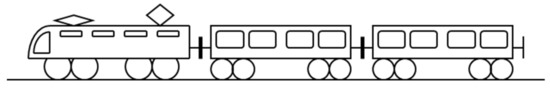 Figure 1. Rolling stock configuration 1: locomotive hauling passenger carriages.
 - railcar convoys based on self-propelled rail vehicles designed to transport passengers which may also travel coupled in multiple units, as shown in Figure 2.
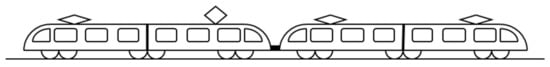 Figure 2. Rolling stock configuration 2: railcars coupled in multiple units.
In the first case (i.e., traditional rail convoys), the unavailability may be related to passenger units or locomotive units. In the case of passenger carriage unavailability where all rail convoys have at least one passenger carriage (see Figure 3b), the number of rail convoys , as well as the planned headway , may be preserved. But a reduction in train capacity of at least one rail convoy entails a reduction in service capacity, , which, in turn, may mean even in ordinary conditions (i.e., without any implementation of ESS) that some passengers may not be able to board the first arriving train arriving, with the direct consequence of an increase in waiting times. In the case of locomotive unavailability, the number of operating rail convoys is generally reduced (see Figure 3c). It entails a reduction in the term which, by means of Equation (1), leads to an increase in planned headway (or equivalently a reduction in service frequency) and hence a reduction in service capacity using Equation (12). In this case, passengers may experience the following:
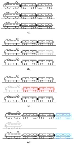
Figure 3.
Service schemes in the case of rolling stock configuration 1: (a) ordinary service; (b) passenger carriage unavailability; (c) locomotive unavailability without carriage reuse; (d) locomotive unavailability with carriage reuse.
- an increase in waiting time due to the increase in headway;
- an increase in crowding levels due to the increase in headway since the number of passengers waiting on the station platform may be calculated as the product between the passenger arrival rate and the service headway (obviously, in the case of variable arrival rate, the above product has to be properly integrated);
- an increase in the probability of not being able to board the first train arriving due to the increase in train occupancy (the service has lower capacity levels ) and an increase in the number of passengers waiting (to board) on the platform. Obviously, in the event of not being able to board the first train, passenger waiting time increases.
The above negative effects may be partially smoothed, as shown in Figure 3d, by using passenger carriages of the faulty train to increase the number of carriages of the operating trains. Obviously, this measure is applicable only if the railway systems (tow ability of locomotives, size of platform/stations, block sections/signalling systems, etc.) allow longer trains to be adopted.
Indeed, in this case, although a smaller number of rail convoys means greater planned headway and hence an increase in waiting times, an increase in train capacity () may preserve the service capacity , thereby avoiding the increase in the number of non-boarding passengers.
On the other hand, concerning the railcar configuration, rolling stock unavailability in the case of a non-intervention strategy (see Figure 4b) entails a reduction in the number of operating rail convoys which, by using Equation (1), implies an increase in planned headway (or equivalently a reduction in service frequency) and hence a reduction in service capacity by means of Equation (12). This condition, as in the case of a traditional train configuration described in Figure 3c, may have adverse effects on passengers in terms of waiting times, crowding levels and number of non-boarding passengers on the first train arriving.
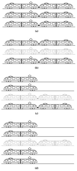
Figure 4.
Service schemes in the case of rolling stock configuration 1: (a) ordinary service; (b) railcar unavailability without any intervention; (c) railcar unavailability with intervention for keeping the number of rail convoys unchanged; (d) railcar unavailability with intervention to increase the number of rail convoys.
In this case, the main intervention for smoothing negative effects is based on reducing the train length by one or more convoys in order to increase the number of operating rail convoys. In particular, two conditions may be identified:
- the number of operating rail convoys is restored (see Figure 4c) so that the planned headway is also restored, according to Equation (1). In this case, passenger waiting time tends to remain unchanged. Obviously, since the service capacity is reduced (due to a reduction in train capacity ), some passengers may not be able to board the first rail convoy arriving, thereby experiencing an increase in waiting time;
- the number of operating convoys is increased (see Figure 4d) with respect to the ordinary condition (shown in Figure 4a). In this case, the planned headway may be reduced according to Equation (1), with the subsequent reduction in passenger waiting times. Obviously, more frequent trains lead to a reduction in crowding levels on platforms. However, as regards the service capacity being calculated with Equation (12), neither a reduction nor an increase can be stated a priori, but a proper simulation model is required for determining its value.
As shown by [20], disruption management may be formulated as a constrained optimisation problem. Our proposal consists of adopting the solution framework proposed by [20] and adapting it in the case of rolling stock unavailability, that is:
subject to:
with:
where is the vector of the strategy implemented to manage the disruption; is the optimal value of ; is the objective function to be minimised; is the vector of user flows perfectly identical to that defined in Equations (13)–(16); is the vector of service parameters, such as running times, which are unaffected by the intervention strategy adopted, unlike the case described by Equations (13)–(16); is the vector of service parameters which are affected by the intervention strategy adopted, unlike the case described by Equations (13)–(16); is the disruption context, which represents rolling stock unavailability; is the assignment function; is the feasibility set of ; is a function which expresses user generalised cost and is the same as that described in Equation (16); is a function which expresses the transport firm’s total cost.
Constraint (18) is theoretically the same as that described by Equation (14), i.e., function is the same as function . The main difference concerns the constant and variable terms: in function (14), parameters such as planned headway (described by ), as well as the rolling stock features (described by ), are fixed while parameters such as running times (described by ) are variable and have to be calculated using the assignment function . By contrast, in function (18), parameters such as running times are fixed (described by ) while parameters such as planned headway (described by ) are variable and have to be calculated through the assignment function . In particular, in this second case, the rolling stock features have to be considered as variables and included in elements of the vector (i.e., ). However, it is worth noting that, in order to provide a realistic simulation (also in terms of energy-saving strategy implementation) in the case of rail system disruptions, as widely shown by [20,22], Constraint (18) has to consider that:
- if passengers at a station platform are not able to board the first arriving train, they have to wait for the subsequent trains by increasing considerably their waiting time [20];
- if this increase in waiting time exceeds certain thresholds, users can choose to leave the rail system to utilise a different transportation system [22].
Constraint (19) provides the feasibility set of the intervention strategies depending on the disruption scenario considered, as described by Figure 3 and Figure 4.
Finally, according to Equation (20), the optimal intervention solution envisages a minimisation of passenger travel costs (i.e., monetarisation of running and waiting times plus possible monetary costs) together with a minimisation of the total costs of the railway service company, which may depend on the intervention policy adopted.
2.4. Joint Management of Rolling Stock Unavailability and ESS Implementation
A further advancement provided in the current paper consists in proposing a methodology for determining the optimal intervention strategy in the case of rolling stock unavailability in the presence of ESS implementation. In particular, our proposal consists of providing a bilevel optimisation framework where:
- the upper level defines the optimal intervention strategy in the case of rolling stock unavailability, as formulated by Equations (17)–(20);
- the lower level is the implementation of an energy-saving strategy which jointly minimises the user generalised cost and energy consumption, as formulated by Equations (13)–(16);
Obviously, each optimisation level has to satisfy service frequency constraints, described by Equations (1)–(11).
A synopsis of the proposed bilevel approach is illustrated in Figure 5.
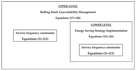
Figure 5.
Framework of the proposed bilevel optimisation problem.
3. Application to a Regional Railway Line
In order to show the utility and feasibility of the proposed approach, we applied it in the case of an Italian regional rail line: the Naples–Sorrento line. This line in southern Italy connects the regional capital (i.e., Naples) with its eastern metropolitan area as far as Sorrento. The main features of the line can be found in [44]. However, the service is performed by railcars called Metrostar (also known as ETR 200) ([46,47]), the capacity of which is 450 passengers, which may be coupled with up to three multiple units, reaching a capacity of 1350 passengers/train.
The first part of the line was inaugurated in 1884. In the following years, the line was gradually extended until 1948, when the town of Sorrento was reached by the service. The current line length is 42.6 km.
Our application was based on the following assumption: the rolling stock consists of 27 railcars, generally coupled in triple-header units. Hence the initial scenario is based on the use of nine rail convoys.
In order to identify the feasibility service configurations, we first considered all combinations of planned headways and number of rail convoys which jointly satisfy Equations (1)–(11). These values are shown in Table 1 and Figure 6. In the case of planned headways between 26.5 and 27.5 min, two different feasible configurations may be identified. Moreover, a preliminary result is that only configurations based on a number of rail convoys belonging to the interval [6,13] may be considered feasible.

Table 1.
Feasible service configurations.
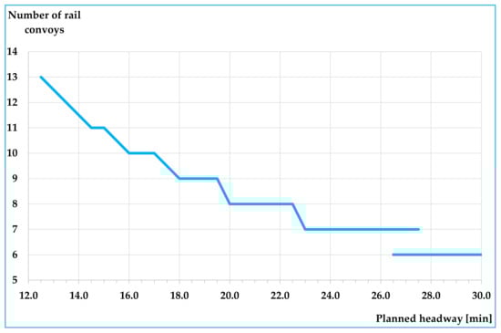
Figure 6.
Feasible service configurations.
A first analysis was performed by adopting coupled schemes (in terms of single-header, double-header and triple-header rail convoys) allowing the use of the ordinary rolling stock endowment (i.e., 27 railcars) to be maximised. By combining all feasible coupled schemes with the feasible number of trains (i.e., interval [6,13]), we obtained the rolling stock scenarios shown in Table 2. Although the current service is implemented by adopting nine triple-header rail convoys, we considered 18 further rolling stock configurations.
Table 2.
Feasible rolling stock combinations in ordinary conditions.
By combining all feasible rolling stock combinations (shown in Table 2) with the feasible service configuration (shown in Table 1), we then identified 30 different service configurations implementable under ordinary conditions, as shown in Table 3.
Table 3.
Service configurations implementable in ordinary conditions.
The current service rolling stock scenario, indicated in Table 2 as A1, may be implemented according to four different operational configurations, indicated in Table 3 as OS1, OS2, OS3 and OS4. Since the rail convoy capacity is 1350 passengers/train, OS4 represents the worst service configuration as it is based on the highest planned headway (i.e., the lowest service frequency). However, by considering all feasible operational schemes, the highest capacity may be achieved in the case of OS5, OS13, OS17 and OS21, where it amounts to 4571 passengers/hour per direction, while the lowest capacity is achieved in the case of OS4, amounting to 4154 passengers/hour per direction.
In Table 3, the worst service configuration is highlighted in red, while the better ones are highlighted in green.
Each service scenario was appropriately simulated in the case of the time-optimal strategy (i.e., all rail convoys were considered at maximum performance levels). Obviously, although this approach entails minimum travel (i.e., running and waiting) times for passengers, it requires maximum energy consumption. Simulation results are indicated in Table 4 where performance parameters were calculated as follows:
where is the running time (i.e., the time spent on the train) associated to the i-th passenger; i is the index identifying the i-th passenger; is the total number of passengers; is the waiting time (i.e., the time spent on the station platform waiting to board the train) associated to the i-th passenger; is the number of railcars of the j-th rail convoy; j is the j-th rail convoy; [] is the number of the outward [return] runs travelled in a day by the j-th rail convoy; [] is the trip length of the outward [return] run; is the objective function adopted in the lower-level problem (i.e., identification of the optimal ESS) being calculated as shown in Equation (16). Obviously, daily energy consumption represents parameter in Equation (16).
Table 4.
Operational parameters in the case of the time-optimal strategy (ordinary conditions).
Our numerical results show that all the scenarios have no reductions in speed limits (i.e., the maximum speed of 90 km/h for both directions) and the same average running time of 32.2 min. The main differences concern waiting times (directly depending on planned headway ) and daily energy consumption (directly depending on daily runs). The worst scenario is OS4 which, although it does not require the maximum energy consumption, experiences the maximum passenger waiting time (average of 9.8 min) and the highest value of the objective function (average of €5.032). Likewise, the optimal scenarios are OS16, OS20, OS24, OS26, OS28, OS29 and OS30 which, despite not requiring minimum energy consumption, benefit from minimum passenger waiting time (average of 6.2 min), implying the lowest value of the objective function (average of €4.322). Finally, although the current scenario (based on rolling stock configuration A1) allows the adoption of uniform vehicles (i.e., all trains consisting in triple-header convoys), it does not represent the best solution. Rather, it presents the worst results in the case of service configuration OS4.
In Table 4, the worst scenario is highlighted in red, while the optimal ones are highlighted in green.
In order to implement the proposed methodology for any service scenario, we carried out energy-saving optimisation, according to Equations (13)–(16), by adopting the following assumptions (i.e., parameters described by vector ):
- the adopted Energy Saving Strategy (ESS) consists in imposing a single speed limit for the outward trip and a single speed limit for the return trip;
- all runs are subjected to the same speed limits;
- the increase in travel times is offset by a reduction in layover times so as to maintain service headway;
- speed limits are imposed so as to maximise the use of layover time (i.e., minimising total energy consumption);
- no energy recovery systems/devices are considered;
- the total layover time may be freely divided between the outward and return trips, according to the theoretical approach proposed by [32].
With the above assumptions, the design variable of the problem (i.e., vector ) may be expressed as follows:
where is the split rate of the total layover time between the outward and return trips (as defined in Section 2.1); [] is the speed limit applied to the outward trip (ot) [return trip (rt)].
Simulation results are reported in Table 5, with CO2 reduction being calculated as follows:
where [] is the energy consumption in the case of a time-optimal strategy [energy saving strategy (ESS)]; is the coefficient which yields energy reductions in terms of CO2 emissions. In particular, by adopting the approach proposed by [48], which analyses CO2 emissions in Italy, the term was considered equal to 0.4889 tons/MWh.
Table 5.
Operational parameters in the case of an energy-saving strategy (ordinary conditions).
The main result is that the proposed approach allows average waiting times to be kept invariable (as can be seen by comparing Table 4 with Table 5). In this case, the reduction in the speed limit entails an increase in passenger running time and a reduction in energy consumption (as well as a reduction in CO2 emissions). Hence the optimal definition of parameter αlt allows the objective function value to be minimised.
The maximum value of the objective function is achieved in the case of scenario OS4, while the minimum value in the case of scenarios OS16, OS20, OS24, OS26, OS26, OS28, OS29 and OS30. In Table 5, the worst scenario is highlighted in red, while the optimal ones are highlighted in green.
However, in order to analyse the effects of ESS implementation, we compared the objective function of each operative scenario with a before-after approach where the ‘before’ condition represents the time-optimal strategy and the ‘after’ condition represents the ESS implementation. These results are shown in Table 6 (obtained by comparing data from Table 3, Table 4 and Table 5), where increases in objective functions (i.e., negative effects in the case of ESS implementation) are indicated in red, while reductions (i.e., positive effects in the case of ESS implementation) are shown in green. However, the main result is that:
Table 6.
Objective function variations in ordinary conditions.
- if a rolling stock scenario can be implemented with a single service configuration, ESS implementation will provide a reduction in objective function value;
- if a rolling stock scenario can be implemented with more than one service configuration, only that with the lower planned headway (i.e., term ) will yield a reduction in objective function value, while the other scenarios will result in an increase in objective function value.
A relevant observation is that rail system operators should adopt, for any rolling stock scenario, only the service scenario with the lowest planned headway, so as to maximise the use of resources.
The second part of the application consisted of introducing the disruption element. We considered a perturbed scenario based on the unavailability of a triple-header rail convoy, so that the total number of operating railcars becomes 24. By way of illustration and for the sake of clarity, what follows is limited to considering only one rolling stock scenario with eight triple-header rail convoys, while complete analysis taking into account all feasible configurations has been shifted to Appendix A.
By analysing the feasible service configurations in the case of eight trains according to Table 1, we obtain six different configurations, as shown in Table 7.
Table 7.
Service configurations implementable in disrupted conditions.
Each service configuration in disrupted conditions was implemented by assuming that the railway service operator may implement three different intervention strategies:
- (1)
- all trains are operated by avoiding any ESS implementation (i.e., all services are performed in time-optimal condition);
- (2)
- all trains are operated by implementing a suitable ESS (i.e., all speed limits are recalculated and applied according to the new rolling stock availability);
- (3)
- all trains are operated by implementing an inappropriate ESS consisting of the speed limits adopted in ordinary conditions (i.e., the railway service operator is unable to update the speed limits promptly).
With the above assumptions, the design variable of the lower level problem is:
and the design variable of the upper-level problem is:
where is the vector of the six service configuration scenarios listed in Table 7, that is:
and is the vector of the above three intervention strategies, that is:
Hence, the feasibility set , consisting of 18 elements, may be expressed as follows:
Moreover, in the case of intervention strategy 3, a rescheduled service may be considered feasible only if the total layover time associated to that scenario (i.e., corresponding value) is no lower than the layover time used in the ordinary condition. Indeed, the adoption of non-updatable speed limits imposes the use of a greater layover time than that effectively available in the disrupted condition, which means that Equations (1)–(11) are no longer satisfied and the frequency-based features of the service cannot be preserved. Hence, element DS1-3 has to be considered unfeasible, that is:
since the in the case of scenario DS1 is 1.55 min, while the layover time used in the reference scenario (scenario OS1 in Table 5) is 3.33 min.
However, due to the limited number of feasible solutions, this kind of problem may be solved by adopting an exhaustive approach (details can be found in [22]).
Numerical results, obtained by considering that the ordinary service is implemented by using nine triple-header rail convoys, are shown in Table 8 and Table 9, grouped by intervention strategy. In particular, Table 8 provides objective function values for any service configuration scenario and for any intervention strategy. Likewise, Table 9 allows for variation in the objective function with respect to the ESS applied in the current condition (i.e., nine triple-header rail convoys).
Table 8.
Intervention scenario evaluation in disrupted conditions.
Table 9.
Intervention scenario improvements in disrupted conditions.
Upon analysing the simulation results, we obtain that the optimal solution is the scenario DS1 with a suitable implementation of ESS, that is:
The main observations are:
- the disrupted condition always yields an increase in objective function value regardless of the strategy adopted due to the discomfort imposed upon passengers;
- the adoption of the optimised ESS always yields an increase in the objective function with respect to the time-optimal condition, except in the case of the lowest planned headway (i.e. scenario DS1);
- the adoption of ESS in the case of nonoptimised speed limits (i.e., the optimal value being calculated in the case of ordinary conditions) always yields an increase in the objective function.
Hence, the main recommendation for the railway service operator in the case of disruption, if speed limits cannot be adjusted for energy-saving reasons, is to remove all limitations (i.e., implement the service in time-optimal conditions) in order to minimise adverse impacts on passengers. Such an intervention strategy allows all service configurations to be implemented, even those with the lowest planned headway, without any limitation due to the availability of total layover time associated to that scenario, so as to minimise passenger waiting times (directly depending on planned headway ). Finally, it is worth implementing an ESS only in the case of the lowest planned headway.
However, a substantial result is that taking passenger costs into account in ESS implementation shows that, in disruption conditions, it is almost always better to give up energy-saving rather than further worsen the travel conditions of passengers.
4. Conclusions and Research Prospects
In this paper, we investigated the implementation of energy-saving strategies (ESS) in the case of constraints in rail rolling stock availability. We analysed the unavailability of rail convoys in a railcar configuration and adopted mitigating interventions consisting in (i) all services being performed in time-optimal conditions; (ii) all services being performed by customising speed limits (i.e., the energy-saving strategy) to the new rolling stock availability; (iii) all services being performed by implementing speed limits adopted in ordinary conditions (i.e., pre-disruption configuration), without updating them according to new rolling stock availability.
The main results showed that, since for each fleet composition it is possible to identify different service configuration scenarios, the optimal strategy always consists in adopting the lowest planned headway. Moreover, in the case of disruption conditions due to rolling stock unavailability, the implementation of ESS is conditional upon the ability of the system manager to update the speed limits in real time. Indeed, if the railway service operator is unable to update speed limits according to the new requirement dictated by the limited rolling-stock configuration, the adoption of a time-optimal condition may represent the winning strategy. On the other hand, in the case of real-time recalculation of speed limits, the implementation of an ESS may provide better results (with respect to the time-optimal) only if the lowest planned headway is adopted.
The stochasticity of the involved variables was considered by adopting proper buffer times for recovering delays. Obviously, a more precise analysis could be developed by using sensitivity analysis techniques (see, for instance, [49]).
Finally, in terms of future research, we propose to analyse different energy-saving measures (such as those based on the use of costing and/or regenerative braking phases) and extend simulation results, as well as the objective function formulation, by allowing for effects of replanning on the primary distribution power grid.
Author Contributions
Conceptualization, L.D.; Data curation, M.B.; Formal analysis, L.D.; Investigation, M.B.; Methodology, L.D.; Validation, M.B. and L.D.; Writing—original draft, M.B. and L.D.; Writing—review and editing, M.B. and L.D. All authors have read and agreed to the published version of the manuscript.
Funding
This research was partially funded by Federico II University of Naples (Italy), grant number 000009-ALTRO-R-2019-LD “Department research DICEA”.
Conflicts of Interest
The authors declare no conflict of interest. The funders had no role in the design of the study; in the collection, analyses or interpretation of data; in the writing of the manuscript, or in the decision to publish the results.
Appendix A
In this Appendix, we extend the disruption results obtained in Section 3 by considering all feasible combinations (in terms of single-header, double-header and triple-header rail convoys) which maximise the use of 24 railcars (disrupted rolling stock endowment), jointly with the feasible number of trains (i.e., interval [6; 13]) as shown in Table A1. In all, we considered 25 rolling stock configurations.
Also in the case of disruption conditions, we combined all feasible rolling stock combinations (shown in Table A1) with the feasible service configuration (shown in Table 1), by identifying 49 different service configurations implementable in disrupted conditions, as shown in Table A2.
Each service configuration in disrupted condition was implemented according to the three intervention strategies described in Section 3. Importantly, also in this case, some elements of SyDM are unfeasible due to values lower than 3.33 min since the non-updatable speed limits require higher values.
Numerical results, shown in Table A3 and Table A4, provide a very similar outcome to the simplified case (i.e., all railcars are coupled in triple-header convoys) described in Section 3. In Table A3 and Table A4, the worst result is shown in red, while the optimal results are indicated in green.
However, a further substantial result is that, in the case of high frequency services (i.e., planned headways equal to 12.5 min), the impact of disruption is so smoothed that even in the case of non-updatable speed limits we obtain lower objective function values (i.e., 4.286 €/pax) even with respect to the ordinary condition (i.e., OS20, OS24, OS26, OS28, OS29 and OS30). Obviously, the elimination of any energy policy allows for further reduction in the objective function (i.e., 4.282 €/pax).
Table A1.
Feasible rolling stock combinations in disrupted conditions.
Table A1.
Feasible rolling stock combinations in disrupted conditions.
| Rolling Stock Scenario | Single-Header Convoys | Double-Header Convoys | Triple-Header Convoys | Total Rail Convoys | Number of Railcars |
|---|---|---|---|---|---|
| B1 | 0 | 0 | 8 | 8 | 24 |
| B2 | 1 | 1 | 7 | 9 | 24 |
| B3 | 3 | 0 | 7 | 10 | 24 |
| B4 | 0 | 3 | 6 | 9 | 24 |
| B5 | 2 | 2 | 6 | 10 | 24 |
| B6 | 4 | 1 | 6 | 11 | 24 |
| B7 | 6 | 0 | 6 | 12 | 24 |
| B8 | 1 | 4 | 5 | 10 | 24 |
| B9 | 3 | 3 | 5 | 11 | 24 |
| B10 | 5 | 2 | 5 | 12 | 24 |
| B11 | 7 | 1 | 5 | 13 | 24 |
| B12 | 0 | 6 | 4 | 10 | 24 |
| B13 | 2 | 5 | 4 | 11 | 24 |
| B14 | 4 | 4 | 4 | 12 | 24 |
| B15 | 6 | 3 | 4 | 13 | 24 |
| B16 | 1 | 7 | 3 | 11 | 24 |
| B17 | 3 | 6 | 3 | 12 | 24 |
| B18 | 5 | 5 | 3 | 13 | 24 |
| B19 | 0 | 9 | 2 | 11 | 24 |
| B20 | 2 | 8 | 2 | 12 | 24 |
| B21 | 4 | 7 | 2 | 13 | 24 |
| B22 | 1 | 10 | 1 | 12 | 24 |
| B23 | 3 | 9 | 1 | 13 | 24 |
| B24 | 0 | 12 | 0 | 12 | 24 |
| B25 | 2 | 11 | 0 | 13 | 24 |
Table A2.
Service configurations implementable in disrupted conditions.
Table A2.
Service configurations implementable in disrupted conditions.
| Service Configuration Scenario | Rolling Stock Scenario | Hplan (min) | NC (#) | TLTTO (min) | Capserv (pax/h) |
|---|---|---|---|---|---|
| DS1 | B1 | 20.0 | 8 | 1.55 | 4050 |
| DS2 | B1 | 20.5 | 8 | 5.55 | 3951 |
| DS3 | B1 | 21.0 | 8 | 9.55 | 3857 |
| DS4 | B1 | 21.5 | 8 | 13.55 | 3767 |
| DS5 | B1 | 22.0 | 8 | 17.55 | 3682 |
| DS6 | B1 | 22.5 | 8 | 21.55 | 3600 |
| DS7 | B2 | 18.0 | 9 | 3.55 | 4000 |
| DS8 | B2 | 18.5 | 9 | 8.05 | 3892 |
| DS9 | B2 | 19.0 | 9 | 12.55 | 3789 |
| DS10 | B2 | 19.5 | 9 | 17.05 | 3692 |
| DS11 | B3 | 16.0 | 10 | 1.55 | 4050 |
| DS12 | B3 | 16.5 | 10 | 6.55 | 3927 |
| DS13 | B3 | 17.0 | 10 | 11.55 | 3812 |
| DS14 | B4 | 18.0 | 9 | 3.55 | 4000 |
| DS15 | B4 | 18.5 | 9 | 8.05 | 3892 |
| DS16 | B4 | 19.0 | 9 | 12.55 | 3789 |
| DS17 | B4 | 19.5 | 9 | 17.05 | 3692 |
| DS18 | B5 | 16.0 | 10 | 1.55 | 4050 |
| DS19 | B5 | 16.5 | 10 | 6.55 | 3927 |
| DS20 | B5 | 17.0 | 10 | 11.55 | 3812 |
| DS21 | B6 | 14.5 | 11 | 1.05 | 4063 |
| DS22 | B6 | 15.0 | 11 | 6.55 | 3927 |
| DS23 | B7 | 13.5 | 12 | 3.55 | 4000 |
| DS24 | B8 | 16.0 | 10 | 1.55 | 4050 |
| DS25 | B8 | 16.5 | 10 | 6.55 | 3927 |
| DS26 | B8 | 17.0 | 10 | 11.55 | 3812 |
| DS27 | B9 | 14.5 | 11 | 1.05 | 4063 |
| DS28 | B9 | 15.0 | 11 | 6.55 | 3927 |
| DS29 | B10 | 13.5 | 12 | 3.55 | 4000 |
| DS30 | B11 | 12.5 | 13 | 4.05 | 3988 |
| DS31 | B12 | 16.0 | 10 | 1.55 | 4050 |
| DS32 | B12 | 16.5 | 10 | 6.55 | 3927 |
| DS33 | B12 | 17.0 | 10 | 11.55 | 3812 |
| DS34 | B13 | 14.5 | 11 | 1.05 | 4063 |
| DS35 | B13 | 15.0 | 11 | 6.55 | 3927 |
| DS36 | B14 | 13.5 | 12 | 3.55 | 4000 |
| DS37 | B15 | 12.5 | 13 | 4.05 | 3988 |
| DS38 | B16 | 14.5 | 11 | 1.05 | 4063 |
| DS39 | B16 | 15.0 | 11 | 6.55 | 3927 |
| DS40 | B17 | 13.5 | 12 | 3.55 | 4000 |
| DS41 | B18 | 12.5 | 13 | 4.05 | 3988 |
| DS42 | B19 | 14.5 | 11 | 1.05 | 4063 |
| DS43 | B19 | 15.0 | 11 | 6.55 | 3927 |
| DS44 | B20 | 13.5 | 12 | 3.55 | 4000 |
| DS45 | B21 | 12.5 | 13 | 4.05 | 3988 |
| DS46 | B22 | 13.5 | 12 | 3.55 | 4000 |
| DS47 | B23 | 12.5 | 13 | 4.05 | 3988 |
| DS48 | B24 | 13.5 | 12 | 3.55 | 4000 |
| DS49 | B25 | 12.5 | 13 | 4.05 | 3988 |
Table A3.
Intervention scenario evaluation in disrupted conditions.
Table A3.
Intervention scenario evaluation in disrupted conditions.
| Service Configuration Scenario | Rolling Stock Scenario | Hplan (min) | NC (#) | Average Objective Function Value | ||
|---|---|---|---|---|---|---|
| (Time Optimal) (€/pax) | (Optimised ESS) (€/pax) | (Non-Optimised ESS) (€/pax) | ||||
| DS1 | B1 | 20.0 | 8 | 5.071 | 5.060 | unfeasible |
| DS2 | B1 | 20.5 | 8 | 5.119 | 5.135 | 5.120 |
| DS3 | B1 | 21.0 | 8 | 5.163 | 5.224 | 5.165 |
| DS4 | B1 | 21.5 | 8 | 5.209 | 5.226 | 5.212 |
| DS5 | B1 | 22.0 | 8 | 5.251 | 5.426 | 5.255 |
| DS6 | B1 | 22.5 | 8 | 5.300 | 5.545 | 5.304 |
| DS7 | B2 | 18.0 | 9 | 4.863 | 4.863 | 4.863 |
| DS8 | B2 | 18.5 | 9 | 4.900 | 4.949 | 4.903 |
| DS9 | B2 | 19.0 | 9 | 4.943 | 5.056 | 4.946 |
| DS10 | B2 | 19.5 | 9 | 4.997 | 5.185 | 5.002 |
| DS11 | B3 | 16.0 | 10 | 4.657 | 4.647 | unfeasible |
| DS12 | B3 | 16.5 | 10 | 4.696 | 4.724 | 4.698 |
| DS13 | B3 | 17.0 | 10 | 4.736 | 4.831 | 4.740 |
| DS14 | B4 | 18.0 | 9 | 4.863 | 4.863 | 4.863 |
| DS15 | B4 | 18.5 | 9 | 4.900 | 4.949 | 4.903 |
| DS16 | B4 | 19.0 | 9 | 4.943 | 5.056 | 4.946 |
| DS17 | B4 | 19.5 | 9 | 4.997 | 5.185 | 5.002 |
| DS18 | B5 | 16.0 | 10 | 4.657 | 4.647 | unfeasible |
| DS19 | B5 | 16.5 | 10 | 4.696 | 4.724 | 4.698 |
| DS20 | B5 | 17.0 | 10 | 4.736 | 4.831 | 4.740 |
| DS21 | B6 | 14.5 | 11 | 4.498 | 4.486 | unfeasible |
| DS22 | B6 | 15.0 | 11 | 4.541 | 4.570 | 4.543 |
| DS23 | B7 | 13.5 | 12 | 4.391 | 4.392 | 4.391 |
| DS24 | B8 | 16.0 | 10 | 4.657 | 4.647 | unfeasible |
| DS25 | B8 | 16.5 | 10 | 4.696 | 4.724 | 4.698 |
| DS26 | B8 | 17.0 | 10 | 4.736 | 4.831 | 4.740 |
| DS27 | B9 | 14.5 | 11 | 4.498 | 4.486 | unfeasible |
| DS28 | B9 | 15.0 | 11 | 4.541 | 4.570 | 4.543 |
| DS29 | B10 | 13.5 | 12 | 4.391 | 4.392 | 4.391 |
| DS30 | B11 | 12.5 | 13 | 4.284 | 4.290 | 4.286 |
| DS31 | B12 | 16.0 | 10 | 4.657 | 4.647 | unfeasible |
| DS32 | B12 | 16.5 | 10 | 4.696 | 4.724 | 4.698 |
| DS33 | B12 | 17.0 | 10 | 4.736 | 4.831 | 4.740 |
| DS34 | B13 | 14.5 | 11 | 4.498 | 4.486 | unfeasible |
| DS35 | B13 | 15.0 | 11 | 4.541 | 4.570 | 4.543 |
| DS36 | B14 | 13.5 | 12 | 4.391 | 4.392 | 4.391 |
| DS37 | B15 | 12.5 | 13 | 4.284 | 4.290 | 4.286 |
| DS38 | B16 | 14.5 | 11 | 4.498 | 4.486 | unfeasible |
| DS39 | B16 | 15.0 | 11 | 4.541 | 4.570 | 4.543 |
| DS40 | B17 | 13.5 | 12 | 4.391 | 4.392 | 4.391 |
| DS41 | B18 | 12.5 | 13 | 4.284 | 4.290 | 4.286 |
| DS42 | B19 | 14.5 | 11 | 4.498 | 4.486 | unfeasible |
| DS43 | B19 | 15.0 | 11 | 4.541 | 4.570 | 4.543 |
| DS44 | B20 | 13.5 | 12 | 4.391 | 4.392 | 4.391 |
| DS45 | B21 | 12.5 | 13 | 4.284 | 4.290 | 4.286 |
| DS46 | B22 | 13.5 | 12 | 4.391 | 4.392 | 4.391 |
| DS47 | B23 | 12.5 | 13 | 4.284 | 4.290 | 4.286 |
| DS48 | B24 | 13.5 | 12 | 4.391 | 4.392 | 4.391 |
| DS49 | B25 | 12.5 | 13 | 4.284 | 4.290 | 4.286 |
The red row identifies the worst service configuration; the green rows identify the better service configurations.
Table A4.
Intervention scenario improvements in disrupted conditions.
Table A4.
Intervention scenario improvements in disrupted conditions.
| Service Configuration Scenario | Rolling Stock Scenario | Hplan (min) | NC (#) | Variation in Average Objective Function Value | ||
|---|---|---|---|---|---|---|
| (Time Optimal) (%) | (Optimised ESS) (%) | (Non-Optimised ESS) (%) | ||||
| DS1 | B1 | 20.0 | 8 | 3.61% | 3.39% | unfeasible |
| DS2 | B1 | 20.5 | 8 | 4.60% | 4.93% | 4.62% |
| DS3 | B1 | 21.0 | 8 | 5.51% | 6.74% | 5.54% |
| DS4 | B1 | 21.5 | 8 | 6.43% | 6.78% | 6.49% |
| DS5 | B1 | 22.0 | 8 | 7.29% | 10.87% | 7.38% |
| DS6 | B1 | 22.5 | 8 | 8.29% | 13.31% | 8.38% |
| DS7 | B2 | 18.0 | 9 | −0.63% | −0.63% | −0.63% |
| DS8 | B2 | 18.5 | 9 | 0.13% | 1.13% | 0.18% |
| DS9 | B2 | 19.0 | 9 | 0.99% | 3.31% | 1.07% |
| DS10 | B2 | 19.5 | 9 | 2.10% | 5.95% | 2.21% |
| DS11 | B3 | 16.0 | 10 | −4.84% | −5.05% | unfeasible |
| DS12 | B3 | 16.5 | 10 | −4.04% | −3.48% | −4.01% |
| DS13 | B3 | 17.0 | 10 | −3.23% | −1.30% | −3.15% |
| DS14 | B4 | 18.0 | 9 | −0.63% | −0.63% | −0.63% |
| DS15 | B4 | 18.5 | 9 | 0.13% | 1.13% | 0.18% |
| DS16 | B4 | 19.0 | 9 | 0.99% | 3.31% | 1.07% |
| DS17 | B4 | 19.5 | 9 | 2.10% | 5.95% | 2.21% |
| DS18 | B5 | 16.0 | 10 | −4.84% | −5.05% | unfeasible |
| DS19 | B5 | 16.5 | 10 | −4.04% | −3.48% | −4.01% |
| DS20 | B5 | 17.0 | 10 | −3.23% | −1.30% | −3.15% |
| DS21 | B6 | 14.5 | 11 | −8.09% | −8.33% | unfeasible |
| DS22 | B6 | 15.0 | 11 | −7.21% | −6.63% | −7.17% |
| DS23 | B7 | 13.5 | 12 | −10.28% | −10.27% | −10.27% |
| DS24 | B8 | 16.0 | 10 | −4.84% | −5.05% | unfeasible |
| DS25 | B8 | 16.5 | 10 | −4.04% | −3.48% | −4.01% |
| DS26 | B8 | 17.0 | 10 | −3.23% | −1.30% | −3.15% |
| DS27 | B9 | 14.5 | 11 | −8.09% | −8.33% | unfeasible |
| DS28 | B9 | 15.0 | 11 | −7.21% | −6.63% | −7.17% |
| DS29 | B10 | 13.5 | 12 | −10.28% | −10.27% | −10.27% |
| DS30 | B11 | 12.5 | 13 | −12.45% | −12.34% | −12.43% |
| DS31 | B12 | 16.0 | 10 | −4.84% | −5.05% | unfeasible |
| DS32 | B12 | 16.5 | 10 | −4.04% | −3.48% | −4.01% |
| DS33 | B12 | 17.0 | 10 | −3.23% | −1.30% | −3.15% |
| DS34 | B13 | 14.5 | 11 | −8.09% | −8.33% | unfeasible |
| DS35 | B13 | 15.0 | 11 | −7.21% | −6.63% | −7.17% |
| DS36 | B14 | 13.5 | 12 | −10.28% | −10.27% | −10.27% |
| DS37 | B15 | 12.5 | 13 | −12.45% | −12.34% | −12.43% |
| DS38 | B16 | 14.5 | 11 | −8.09% | −8.33% | unfeasible |
| DS39 | B16 | 15.0 | 11 | −7.21% | −6.63% | −7.17% |
| DS40 | B17 | 13.5 | 12 | −10.28% | −10.27% | −10.27% |
| DS41 | B18 | 12.5 | 13 | −12.45% | −12.34% | −12.43% |
| DS42 | B19 | 14.5 | 11 | −8.09% | −8.33% | unfeasible |
| DS43 | B19 | 15.0 | 11 | −7.21% | −6.63% | −7.17% |
| DS44 | B20 | 13.5 | 12 | −10.28% | −10.27% | −10.27% |
| DS45 | B21 | 12.5 | 13 | −12.45% | −12.34% | −12.43% |
| DS46 | B22 | 13.5 | 12 | −10.28% | −10.27% | −10.27% |
| DS47 | B23 | 12.5 | 13 | −12.45% | −12.34% | −12.43% |
| DS48 | B24 | 13.5 | 12 | −10.28% | −10.27% | −10.27% |
| DS49 | B25 | 12.5 | 13 | −12.45% | −12.34% | −12.43% |
The red row identifies the worst service configuration; the green rows identify the better service configurations.
References
- Cartenì, A. Accessibility indicators for freight transport terminals. Arab. J. Sci. Eng. 2014, 39, 7647–7660. [Google Scholar] [CrossRef]
- Cartenì, A. Urban sustainable mobility. Part 1: Rationality in transport planning. Transp. Probl. 2014, 9, 39–48. [Google Scholar]
- Cartenì, A. Urban sustainable mobility. Part 2: Simulation models and impacts estimation. Transp. Probl. 2015, 10, 5–16. [Google Scholar] [CrossRef]
- Gallo, M. The impact of urban transit systems on property values: A model and some evidences from the city of Naples. J. Adv. Transp. 2018, 2018, 1767149. [Google Scholar] [CrossRef]
- Gallo, M. Improving equity of urban transit systems with the adoption of origin-destination based taxi fares. Socio-Econ. Plan. Sci. 2018, 64, 38–55. [Google Scholar] [CrossRef]
- CENELEC. EN 50126-1: Railway Applications—Specification and Demonstration of Reliability, Availability, Maintainability and Safety (RAMS); European Committee for Electrotechnical Standardization: Brussels, Belgium, 1999. [Google Scholar]
- International Electrotechnical Commission (IEC). IEC 61508: Functional Safety of Electrical/Electronic/Programmable Electronic Safety-Related Systems—Part 4: Definitions and Abbreviations; International Electrotechnical Commission: Genève, Switzerland, 2001. [Google Scholar]
- Medeiros, G. RAMS Analysis of Railway Track Infrastructure. Master’s Thesis, University of Lisbon, Lisbon, Portugal, 2008. [Google Scholar]
- Patra, A.P. Maintenance Decision Support Models for Railway Infrastructure Using RAMS & LCC Analyses. Ph.D. Thesis, Luleå University of Technology, Luleå, Sweden, 2009. [Google Scholar]
- Park, M.G. RAMS Management of Railway Systems. Ph.D. Thesis, University of Birmingham, Birmingham, UK, 2013. [Google Scholar]
- Pandey, A.K. RAMS management for a complex railway system: A case study. In Proceedings of the 2014 International Applied Reliability Symposium, Bangalore, India, 12–14 November 2014. [Google Scholar]
- Praticò, F.; Giunta, M. An integrative approach RAMS-LCC to support decision on design and maintenance of rail track. In Proceedings of the 10th International Conference Environmental Engineering, Vilnius, Lithuania, 27–28 April 2017. [Google Scholar]
- Mahboob, Q.; Zio, E. Handbook of RAMS in Railway Systems: Theory and Practice; CRC Press by Taylor & Francis Group: Boca Raton, FL, USA, 2018. [Google Scholar]
- Louwerse, I.; Huisman, D. Adjusting a railway timetable in case of partial or complete blockades. Eur. J. Oper. Res. 2014, 235, 583–593. [Google Scholar] [CrossRef]
- Zhan, S.; Kroon, L.; Veelenturf, L.P.; Wagenaar, J.C. Real-time high-speed train rescheduling in case of a complete blockage. Transport. Res. B-Meth. 2015, 78, 182–201. [Google Scholar] [CrossRef]
- Durmus, M.S.; Takai, S.; Söylemez, M.T. Fault diagnosis in fixed-block railway signaling systems: A discrete event systems approach. IEEJ Trans. Electr. Electron. 2014, 9, 523–531. [Google Scholar] [CrossRef]
- Botte, M.; D’Acierno, L.; Montella, B.; Placido, A. A stochastic approach for assessing intervention strategies in the case of metro system failures. In Proceedings of the 2015 AEIT International Annual Conference, Naples, Italy, 14–16 October 2015. [Google Scholar]
- Botte, M.; Puca, D.; Montella, B.; D’Acierno, L. An innovative methodology for managing service disruptions on regional rail lines. In Proceedings of the 10th International Conference Environmental Engineering, Vilnius, Lithuania, 27–28 April 2017. [Google Scholar]
- Hao, W.; Meng, L.; Veelenturf, L.P.; Long, S.; Corman, F.; Niu, X. Optimal reassignment of passengers to trains following a broken train. In Proceedings of the 2018 IEEE International Conference on Intelligent Rail Transport (IEEE ICIRT 2018), Marina Bay Sands, Singapore, 12–14 December 2018. [Google Scholar]
- D’Acierno, L.; Gallo, M.; Montella, B.; Placido, A. The definition of a model framework for managing rail systems in the case of breakdowns. In Proceedings of the 16th International IEEE Conference on Intelligent Transportation Systems (IEEE ITSC 2013), The Hague, The Netherlands, 6–9 October 2013. [Google Scholar]
- D’Acierno, L.; Placido, A.; Botte, M.; Gallo, M.; Montella, B. Defining robust recovery solutions for preserving service quality during rail/metro systems failure. Int. J. Supply Oper. Manag. 2016, 3, 1351–1372. [Google Scholar]
- D’Acierno, L.; Placido, A.; Botte, M.; Montella, B. A methodological approach for managing rail disruptions with different perspectives. Int. J. Math. Models Methods Appl. Sci. 2016, 10, 80–86. [Google Scholar]
- Caprara, A.; Kroon, L.; Monaci, M.; Peeters, M.; Toth, P. Passenger Railway Optimization. In Handbooks in Operations Research and Management Science; North Holland Publishing Company: North Holland, The Netherlands, 2007; Volume 14, pp. 129–187. [Google Scholar]
- Chuang, H.J.; Chen, C.S.; Lin, C.H.; Hsieh, C.H.; Ho, C.Y. Design of optimal coasting speed for saving social cost in mass rapid transit systems. In Proceedings of the 3rd International Conference on Deregulation and Restructuring and Power Technologies (DRPT 2008), Nianjing, China, 6–9 April 2008. [Google Scholar]
- De Martinis, V.; Weidmann, U.; Gallo, M. Towards a simulation-based framework for evaluating energy-efficient solutions in train operation. WIT Trans. Built Environ. 2014, 135, 721–732. [Google Scholar]
- D’Acierno, L.; Botte, M.; Montella, B. An analytical approach for determining reserve times on metro systems. In Proceedings of the 17th IEEE International Conference on Environment and Electrical Engineering (IEEE EEEIC 2017) and 1st Industrial and Commercial Power Systems Europe (I&CPS 2017), Milan, Italy, 6–9 June 2017. [Google Scholar]
- Guastafierro, A.; Lauro, G.; Pagano, M.; Roscia, M. A method for optimizing coasting phases in railway speed profiles: An application to an Italian route. In Proceedings of the 2016 International Conference on Electrical Systems for Aircraft, Railway, Ship Propulsion and Road Vehicles & International Transportation Electrification Conference (ESARS ITEC 2016), Toulouse, France, 2–4 November 2016. [Google Scholar]
- Keskin, K.; Karamancioglu, A. Energy efficient motion control for a light rail vehicle using the big bang big crunch algorithm. IFAC-PapersOnLine 2016, 49, 442–446. [Google Scholar] [CrossRef]
- Scheepmaker, G.; Goverde, R.M.P. The interplay between energy-efficient train control and scheduled running time supplements. J. Rail Transp. Plan. Manag. 2015, 5, 225–239. [Google Scholar] [CrossRef]
- Wang, P.; Goverde, R.M.P. Multi-train trajectory optimization for energy-efficient timetabling. Eur. J. Oper. Res. 2019, 272, 621–635. [Google Scholar] [CrossRef]
- Botte, M.; D’Acierno, L. Dispatching and rescheduling tasks and their interactions with travel demand and the energy domain: Models and algorithms. Urban Rail Transit 2018, 4, 163–197. [Google Scholar] [CrossRef]
- D’Acierno, L.; Botte, M.; Gallo, M.; Montella, B. Defining reserve times for metro systems: An analytical approach. J. Adv. Transp. 2018, 2018, 5983250. [Google Scholar] [CrossRef]
- Gonzalez-Gil, A.; Palacin, R.; Batty, P. Sustainable urban rail systems: Strategies and technologies for optimal management of regenerative braking energy. Energy Convers. Manag. 2013, 75, 374–388. [Google Scholar] [CrossRef]
- Kim, K.M.; Kim, K.T.; Han, M.S. A model and approaches for synchronized energy saving in timetabling. In Proceedings of the 9th World Congress on Railway Research (WCRR 2011), Lille, France, 22–26 May 2011. [Google Scholar]
- Yang, X.; Li, X.; Gao, Z.; Wang, H.; Tang, T. A cooperative scheduling model for timetable optimization in subway systems. IEEE Trans. Intell. Transp. 2013, 14, 438–447. [Google Scholar] [CrossRef]
- Cornic, D. Efficient recovery of braking energy through a reversible dc substation. In Proceedings of the Electrical Systems for Aircraft, Railway and Ship Propulsion (ESARS 2010), Bologna, Italy, 19–21 October 2010. [Google Scholar]
- Ibaiondo, H.; Romo, A. Kinetic energy recovery on railway systems with feedback to the grid. In Proceedings of the 14th International Power Electronics and Motion Control Conference (EPE-PEMC 2010), Ohrid, Macedonia, 6–8 September 2010. [Google Scholar]
- Romo, L.; Turner, D.; Ng, L.S.B. Cutting traction power costs with wayside energy storage systems in rail transit systems. In Proceedings of the 2005 Joint Rail Conference (JRC 2005), Pueblo, CO, USA, 16–18 March 2005. [Google Scholar]
- Ghavihaa, N.; Campilloa, J.; Bohlinb, M.; Dahlquista, E. Review of application of energy storage devices in railway transportation. Energy Proced. 2017, 105, 4561–4568. [Google Scholar] [CrossRef]
- Iannuzzi, D.; Tricoli, P. Speed-based state-of-charge tracking control for metro trains with onboard supercapacitors. IEEE Trans. Power Electr. 2012, 27, 2129–2140. [Google Scholar] [CrossRef]
- Song, R.; Yuan, T.; Yang, J.; He, H. Simulation of braking energy recovery for the metro vehicles based on the traction experiment system. Simulation 2017, 93, 1099–1112. [Google Scholar]
- Fallah, M.; Asadi, M.; Moghbeli, H.; Dehnavi, G.R. Energy management and control system of DC-DC converter with super-capacitor and battery for recovering of train kinetic energy. J. Renew. Sustain. Energy 2018, 10, 0174103. [Google Scholar] [CrossRef]
- D’Acierno, L.; Botte, M. The implementation of energy-saving strategies in the case of limitation in rolling stock availability. In Proceedings of the 19th IEEE International Conference on Environment and Electrical Engineering (IEEE EEEIC 2019) and 3rd Industrial and Commercial Power Systems Europe (I&CPS 2019), Genoa, Italy, 11–14 June 2019; pp. 380–385. [Google Scholar]
- D’Acierno, L.; Botte, M. A passenger-oriented optimization model for implementing energy-saving strategies in railway contexts. Energies 2018, 11, 2946. [Google Scholar] [CrossRef]
- International Union of Railways (UIC). UIC CODE 451-1: Timetable Recovery Margins to Guarantee Timekeeping—Recovery Margins; UIC: Paris, France, 2000. [Google Scholar]
- Pezzillo Iacono, M.; Martinez, M.; Mangia, G.; Galdiero, C. Knowledge creation and inter-organisational relationships: The development of innovation in the railway industry. J. Knowl. Manag. 2012, 16, 604–616. [Google Scholar] [CrossRef]
- Mariscotti, A.; Marrese, A.; Pasquino, N.; Schiano Lo Moriello, R. Time and frequency characterization of radiated disturbance in telecommunication bands due to pantograph arcing. Measurement 2013, 46, 4342–4352. [Google Scholar] [CrossRef]
- Caputo, A. Affecting atmospheric emissions of CO2 and other greenhouse gases within the electricity industry (In Italian). In Technical Report 257/2017, National Institute for Environmental Protection and Research; ISPRA: Rome, Italy, 2017. [Google Scholar]
- Saltelli, A.; Ratto, M.; Andres, T.; Campolongo, F.; Cariboni, J.; Gatelli, D.; Saisana, M.; Tarantola, S. Global Sensitività Analysis: The Primer; John Wiley & Sons Ltd.: Chichester, UK, 2008. [Google Scholar]


© 2020 by the authors. Licensee MDPI, Basel, Switzerland. This article is an open access article distributed under the terms and conditions of the Creative Commons Attribution (CC BY) license (http://creativecommons.org/licenses/by/4.0/).