Novel Adsorption Cycle for High-Efficiency Adsorption Heat Pumps and Chillers: Modeling and Simulation Results

Abstract

A novel thermodynamic cycle for adsorption heat pumps and chillers is presented. It shows a significant improvement of the internal heat recovery between the adsorption and the desorption half cycle. A stratified thermal storage, which allows for a temperature-based extraction and insertion of storage fluid, is hydraulically coupled with a single adsorber. The benefit is an increased efficiency by reusing the released heat of adsorption for regeneration of the adsorber and by rendering possible low driving temperature differences. For investigating the second law of this cycle, a dynamic model is employed. The transient behavior of the system and the respective losses because of driving temperature differences at the heat exchangers and losses due to mixing within the storage and to the surroundings are depicted in this one-dimensional model. The model is suitable both for analyzing this advanced cycle as well as for comparisons with other cycles.

1. Introduction

Typical coefficients of performance ($COP$) attainable employing a standard adsorption heat pump cycle are significantly lower than those using a standard single stage absorption cycle [1]. The reasons are the nonsteady temperature swing of the adsorbers and of the corresponding piping as well as the inferior internal heat recovery compared to that of an absorption cycle realized using a solution heat exchanger. Adsorption cycles allowing for the recovery of a large fraction of internal heat may lead to improved efficiencies. A heating $COP$ even beyond 2 is possible, if sorptive and not only sensible heat is recovered. In previous papers [2,3,4], a number of such advanced cycles have been proposed and analyzed. However, none of them has been employed for building commercial devices for two main reasons: the hydraulic circuits required as well as the control strategies being relatively complex.

In this paper, a novel advanced adsorption cycle is presented in its basic setup employing a single adsorber only. Although the authors believe the cycle to be simple enough to favor a commercial development, the integration of a stratified thermal storage leads to a significantly improved performance. The storage tank is hydraulically connected to the adsorber, and the heat transfer fluid (HTF) employed serves as the storage fluid in the tank simultaneously, avoiding heat exchangers and the corresponding losses. Sensible and latent heat is stored during adsorption and reused during desorption later, which reduces the amount of required driving heat.

While some aspects of this novel cycle were presented before at conferences [5,6,7,8,9], this paper focuses on a comprehensive discussion of the modeling and simulation aspects of the cycle and on results for a heat pump application. The Ph.D. thesis of the first author does comprise a more rigorous description of the (transient) model. It also includes the consideration of other adsorbents (namely SAPO-34) and configurations and the same and other results and evaluations [10] (in German).

The model employed for the analysis of this system was developed with the main goals of combining accuracy regarding the main physical effects with numerical efficiency and thermodynamic consistency. System-level models of adsorption heat pumps (and chillers) described in literature [11,12] still mostly employ single node (0D) models of the heat exchangers.

A numerical plug flow model comprising one-dimensionally resolved adsorber and storage components was developed in order to simulate a system employing this new adsorption cycle. The model and a corresponding system are described in the following sections. The performance of the cycle and of the system is analyzed stationarily and through transient simulations using the presented model. The focus is on the working pair water–zeolite Li-Y [13], which allows for a large temperature overlap of the differential heats of adsorption and desorption but requires maximal driving temperatures of up to 220 ${}^{\circ }\mathrm{C}$. Correspondingly, thermal oil should be employed and is considered here as the HTF.

Figure 1a shows the differential heats of adsorption and desorption for this working pair, for our set of assumptions on thermal masses (cf. shown in the table below in Section 4.1.1), for a minimal adsorber/condenser temperature of 34${}^{\circ }\mathrm{C}$ and an evaporator temperature of 8 ${}^{\circ }\mathrm{C}$. These differential heat curves are derived from a pure adsorption equilibrium model integrated over an ideal cycle with two isobars and two isosteres (cf. [10] (Section 3.2), [8,14]).

The overlap of the heat curves (violet area in Figure 1a) represents the maximal recoverable heat for this working pair under the given temperature and thermal mass conditions. The remaining required heat of desorption (with ideal heat recovery) and the remaining excess heat of adsorption (not useful for heat recovery) are indicated in Figure 1a as thin red and blue lines. It is understood from these heat curves that the recoverable heat is maximized for adsorption and desorption curves smoothed out over a large temperature range. However, when searching for novel adsorbents for standard adsorption cycles (which are not suitable to achieve a high internal heat recovery), an S-shaped adsorption isotherm is desired [13,16,17]. This leads to sharper peaks in the differential heat curves and thus a reduced temperature overlap and recoverable heat. Therefore, the advantage of any cycle allowing for a large internal heat recovery over a standard two-adsorber cycle can be expected to be higher for the type of working pair with a loading field stretched evenly across a wide temperature range (that is linear rather than S-shaped isotherms and isobars).

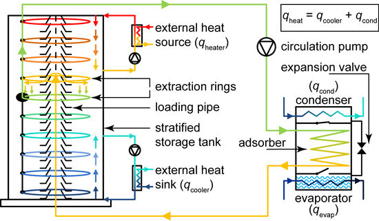
2. The Stratisorp System

2.1. Cycle Concept and Storage Integration

The key concept of the Stratisorp cycle is the integration of a well-insulated stratified thermal storage tank in the adsorption cycle. The temperature of the fluid increases with the height of the storage, such that buoyancy forces caused by the temperature-dependent fluid density counteract convection within the tank. The extraction of fluid of a desired temperature as well as the injection of fluid at heights corresponding to its temperature is required for a beneficial usage. For this purpose, a number of extraction rings are distributed along the height of storage. Using a multi-way valve, they are used for extracting fluid of a given temperature. Furthermore, the storage is equipped with an insertion pipe that allows for a passive temperature-specific injection. Alternatively, the extraction rings could be used for fluid insertion as well when using a second multi-way valve for the return flow into the tank.

During adsorption, the adsorber must be cooled down. Fluid is extracted from the storage at successively lower extraction rings that access fluid at temperatures always a little lower than that of the adsorber. The goal is to remove the heat from the adsorber with low driving temperature differences. The heat is transferred to the HTF, which then returns to the stratified storage and is inserted at heights corresponding to its temperatures. As the adsorber is cooled down, the returning fluid is inserted above the extraction ring that the fluid is extracted from simultaneously. As a result, the temperature profile over the storage height at the start of adsorption is shifted to higher temperatures by the stored heat. In an idealized case, the temperature offset is almost independent of the storage height.

Correspondingly, during desorption, the adsorber must be heated. Fluid is extracted at subsequently greater heights, again considering a low driving temperature difference. The temperature profile within the storage is moved back down to its original state. Heat newly added by the driving source must be used to regenerate the adsorber not before the last phase of the cycle. In this manner, a large fraction of the sensible and latent heat stored during adsorption can be reused during desorption. However, the adsorption equilibria of the chosen working pair and the heat and mass transfer characteristics of the adsorber have a large influence on the amount of heat recovered internally.

In previous work [18], it was shown that the irreversibilities due to external temperature coupling considerably limit the efficiency of the standard adsorption cycle. Using low driving temperature differences, these irreversibilities can be considerably reduced, at the cost of new irreversibilities introduced by convective mixing within the storage and longer cycle times, given an adsorber of the same heat transfer characteristics.

In an advanced cycle concept introduced previously [2], a large number of adsorbers are hydraulically switched in such a manner that a cyclic permutation of adsorbers along the heat transfer loop is achieved. Thus, heat of adsorption from adsorbers on the adsorption branch of the cycle is transferred to adsorbers on the desorption branch of the cycle. The key difference between this multi-adsorber cycle and the Stratisorp cycle is that in the former, all phases of the cycle occur simultaneously in different adsorbers, that is for each adsorber in a certain temperature window on the adsorption branch, an adsorber on the desorption branch can be found to which it can transfer heat. In the Stratisorp cycle, the phases of the cycle are temporally separated; heat from each temperature window is stored separately in the storage until it is needed in the next half cycle. In this way, internal heat recovery can be realized with a single adsorber.

2.2. Adsorber Design

Compared to a standard adsorption cycle, the typical driving temperature differences occurring for the Stratisorp cycle are considerably smaller. Hence, innovative adsorber concepts with improved characteristics regarding heat and—to a smaller extent—mass transfer are required to derive full advantage from this cycle. Within this paper, an aluminum plate type adsorber comprising a large number of extruded fluid channels with correspondingly small diameters is considered. In this manner, the heat transfer between the fluid and the heat exchanger is improved considerably. The adsorber design is still under development [19,20,21], particularly regarding the manufacturing process, e.g., the joining technology, the channel layout, as well as the interconnection of the modules. Aluminum fiber structures are sintered on top of the heat exchanger plates, and these structures are assumed to be coated with the adsorbent zeolite Li-Y. The thickness of the coating is about 30 µm, and that of the fiber structure is about 3.5 mm. However, the heat transfer characteristics are improved at the expense of the ratio of latent to sensible heat, both compared to a conventional packed-bed adsorber. The adsorber design is shown in Figure 1b.

2.3. Heater and Cooler

By coupling the driving heat source to the upper region of the storage tank and the heat rejection loop to its lower region, a large temperature spread in both of these external heat flows can be achieved. This is a key advantage of this concept. Furthermore, both devices can operate continuously, resulting in lower losses corresponding to the heat exchangers and steadier utilization of the heat sources and sinks. In this manner, the storage serves a second purpose as a buffer storage for driving heat and for heat to be delivered to the medium-temperature sink.

3. Description of the Model

The model comprises two main parts: the adsorber and the storage component. Both are modeled one-dimensionally, and they are coupled by a hydraulic circuit. The corresponding heat transfer fluid (HTF) is modeled as an ideal (fractional) plug flow.

3.1. Adsorber, Evaporator, and Condenser

The adsorber model is discretized into n nodes in flow direction of the HTF. Before and after these adsorber nodes, one additional pipe node represents the piping between the adsorber and the storage as well as the piping connecting the adsorber elements, respectively.

The adsorber nodes incorporate the mass of the heat exchanger and the adsorbent as well as that of the adsorbate. The nodes can exchange heat with the HTF within the heat exchanger, with the neighboring adsorber nodes and with the adsorptive (i.e., the working fluid, which is modeled as a real gas) within the adsorber chamber. Furthermore, heat loss via the housing to evaporator and condenser is considered. The adsorption enthalpy related to the amount adsorbed or desorbed is added to or removed from the corresponding adsorber nodes. For the adsorption half cycle, the heat for superheating the vapor from the evaporator to the adsorber temperature is taken from the respective adsorber nodes. The heat released for cooling down the desorbed vapor from the adsorber to the condenser temperature is added to the condenser during the desorption half cycle. The valves separating the adsorber chamber from evaporator and condenser are closed at the beginning of each half cycle. They open when the pressure in the adsorber chamber dropped to that in the evaporator (adsorption) or increased to that in the condenser (desorption).

The energy balance of the adsorber states as

$$\begin{array}{cc}\hfill & \frac{1}{n}\sum _{i=1}^n\left(m_{\mathrm{hx}}{c}_{\mathrm{hx}}+m_{\mathrm{s}}\left(c_{\mathrm{s}}+x_i{c}_{x_i,\mathrm{a}}(T_i)\right)\right)\frac{d{T}_i}{dt}{\widehat{\mathit{u}}}_i\hfill \\ \hfill & ={\dot{\mathit{Q}}}_{}+\frac{m_{\mathrm{s}}}{n}\sum _{i=1}^n\frac{d{x}_i}{dt}{\widehat{\mathit{u}}}_i\left\{\begin{array}{cc}{q}_{\mathrm{st}}(x_i,T_i)-\left(h_{\mathrm{g}}(p_i,T_i)-h_{\mathrm{g}}(p_{\mathrm{c}},T_{\mathrm{c}})\right),\hfill & \mathrm{adsorption},\hfill \\ q_{\mathrm{st}}(x_i,T_i),\hfill & \mathrm{desorption},\hfill \end{array}\right.\hfill \end{array}$$

(1)

where ${\widehat{\mathit{u}}}_i$ is the i. canonical unit vector and $T_i$ and $x_i$ are the temperature and the loading of the ith adsorber node, respectively. The left hand side of (1) describes the change in energy of the adsorber nodes when temperature changes, which corresponds to their thermal capacity, and the second term on the right hand side describes the heat released or removed due to the mass flow of the working fluid, respectively.

The thermal capacity of each adsorber node comprises the proportional capacity of the heat exchanger $m_{\mathrm{hx}}{c}_{\mathrm{hx}}/n$, that of the adsorbent $m_{\mathrm{s}}{c}_{\mathrm{s}}/n$, and that of the current amount adsorbed $m_{\mathrm{s}}{x}_i{c}_{x_i,\mathrm{a}}(T_i)/n$.

The adsorbed phase heat capacity $c_{x_i,\mathrm{a}}(T)$ depends on amount adsorbed and temperature. The determination of this heat capacity and of the adsorption enthalpy $q_{\mathrm{st}}(x_i,T_i)$ is done as described in [22]. The characteristic curve required in the methodology of Dubinin [23] and used within this paper is fitted according to Gaussian process regression according to [24] and given in [10] (pp. 190–191). This fitting method of Dubinin’s characteristic curve leads to a good fit to measured adsorption equilibrium data while it avoids overfitting of these data that may occur with some alternative fitting methods [24]. The selected hyperparameters of the Gaussian process are given in

Table 1. Hyperparameters for the fit of equilibrium loading of the working pair water–zeolite Li-Y using Gaussian process regression [24].

Hyperparameter	Value
l	1186.9
${\sigma }_f^2$	2.7416 × 10−4
${\sigma }_0^2$	4.3911 × 10−6

. The material data of the working pair is described in [13]. The properties of the working fluid (water) is computed from [25].

The energy and entropy residuals of the adsorption module and of the storage vanish compared to the numerical accuracy, despite the highly dynamical characteristic of the Stratisorp cycle, the large storage, and the real gas consideration. This is due to the consistent modeling of adsorbed phase heat capacity and adsorption enthalpy, as well as to the rigorous derivation and consideration of all energy and entropy terms from the first law.

3.1.1. Adsorber Heat Flow

The total heat flow ${\dot{\mathit{Q}}}_{}$ in (1) comprises that to the HTF plus some loss flows:

$$\begin{array}{cc}\hfill {\dot{\mathit{Q}}}_{}& =-{\dot{\mathit{Q}}}_{1n}^{\mathrm{htf}}+\frac{{\lambda }_{\mathrm{eff}}^{\perp }{A}_{\mathrm{hx}}^{\perp }}{l/n}({\mathit{T}}_{11}-2\mathit{T}+{\mathit{T}}_{nn})-\frac{{(hA)}_{\mathrm{c}}}{n}(\mathit{T}-T_{\mathrm{c}}\mathbf{1})+\frac{{(UA)}_{\mathrm{h}}}{n}(T_{\mathrm{ev}}\mathbf{1}+T_{\mathrm{cd}}\mathbf{1}-2\mathit{T}),\hfill \end{array}$$

(2)

where $\mathit{T}$ is the temperature vector of the adsorber nodes, ${\mathit{T}}_{11}={(T_1,T_1,T_2,\cdots ,T_{n-1})}^{\top }$, ${\mathit{T}}_{nn}={(T_2,T_3,\cdots ,T_n,T_n)}^{\top }$, and ${\dot{\mathit{Q}}}_{1n}^{\mathrm{htf}}={({\dot{Q}}_1^{\mathrm{htf}},\cdots ,{\dot{Q}}_n^{\mathrm{htf}})}^{\top }$. The right hand side terms are discussed in detail below.

The heat flow from the n adsorber as well as that from the two pipe nodes to the corresponding fluid plugs of the HTF ${\dot{\mathit{Q}}}_{1n}^{\mathrm{htf}}$ is computed according to a standard NTU heat exchanger model [26] as

$${\dot{\mathit{Q}}}_{1n}^{\mathrm{htf}}=\dot{m}{c}_{\mathrm{htf}}\sum _{i=0}^{n+1}{ϵ}_i(T_i-T_i^{\mathrm{htf}}){\widehat{\mathit{u}}}_i,\mathrm{where}{ϵ}_i=1-exp\left(-\frac{U_{\mathrm{hx}}(T_i)A_{\mathrm{hx}}}{\dot{m}{c}_{\mathrm{htf}}n}\right),$$

(3)

where the indices 0 and $n+1$ indicate the two pipe nodes before and after the n adsorber nodes as well as the corresponding fluid plugs. They represent the pipes between the storage and the adsorber as well as the pipes connecting the modules within the adsorber (parasitic thermal mass) but they do not accurately represent the fluid volume in the pipes and its circulation time, since the pipe nodes’ fluid volume is equal to that of the adsorber nodes.

Due to their small diameter, the flow within the channels is laminar, and the Nußelt number can be computed ($0<\mathit{Re}\mathit{Pr}d/l<\infty$) (see [27] (p. 694)) to be ${\mathit{Nu}}_{\mathrm{lam}}={\{{\mathit{Nu}}_1^3+{0.7}^3+{[{\mathit{Nu}}_2-0.7]}^3\}}^{1/3}$, where ${\mathit{Nu}}_1=3.66$ and ${\mathit{Nu}}_2=1.615\sqrt[3]{\mathit{Re}\mathit{Pr}(d/l)}$. Hence, the heat transfer from the HTF to the pipe surface can be described by $h=\mathit{Nu}\lambda /d$, where d is the channel diameter and $\lambda$ the thermal conductivity of the fluid, while assuming a constant surface temperature of the pipe.

3.1.2. Effective Adsorber Thickness

Furthermore, besides h, the overall heat transfer coefficient $U_{\mathrm{hx}}=1/(1/h+l_{\mathrm{eff}}/\lambda )$ comprises the heat conduction through the adsorbent. In the following, the effective thickness $l_{\mathrm{eff}}$ is estimated.

For the ith adsorber node, the average adsorbent temperature $T_i$ is computed over dimension x, which is perpendicular to the direction z of the HTF flow, to be $T_i=\overline{T}(z_i)=D^{-1}{\int }_x^{D}dxT(x)$. With this effective temperature, a simple effective model is ${\dot{q}}_0^i=-\lambda (T_i-T_{\mathrm{wall}})/l_{\mathrm{eff}}$, where ${\dot{q}}_0\equiv \dot{q}(x=0)$ is the total heat flux, $T_{\mathrm{wall}}\equiv T(x=0)$ the temperature at the fluid pipes, and $l_{\mathrm{eff}}$ the yet unknown effective thickness. The latter is then used for computing the effective overall heat transfer coefficient $U_{\mathrm{hx}}$ above.

Assuming that the amount adsorbed and correspondingly the adsorption enthalpy released or absorbed is constant over the adsorbent thickness (i.e., along x)—which is not reasonable for short times, but for full half cycles—the heat flux is proportional to the distance from the pipe surface at $x=D$ and states $\dot{q}(x)={\dot{q}}_0(1-x/D)$. Employing this linear equation and Fourier’s law $-\lambda dT/dx=\dot{q}$, the temperature profile can be easily computed by separation of variables:

$$\begin{array}{cc}\hfill {\int }_{T(0)\equiv T_{\mathrm{wall}}}^{T(x)}dT& =\frac{-1}{\lambda }{\int }_0^{x}d{x}^{\prime }{\dot{q}}_0\left(1-\frac{x^{\prime }}{D}\right)\Rightarrow T(x)=T_{\mathrm{wall}}+\frac{-{\dot{q}}_0}{\lambda }\left(x-\frac{x^2}{2D}\right).\hfill \end{array}$$

(4)

The average temperature is given by $\overline{T}=D^{-1}{\int }_0^{D}dxT(x)=T_{\mathrm{wall}}-\frac{{\dot{q}}_{0}D}{3\lambda }$. Rearranging the simple model above leads to $l_{\mathrm{eff}}=-\lambda (\overline{T}-T_{\mathrm{wall}})/{\dot{q}}_0$. Plugging in $\overline{T}$ from above yields the effective thickness $l_{\mathrm{eff}}=D/3$ [10] (Section 4.3.2).

3.1.3. Lateral Heat Conduction in Adsorber

Each adsorber node exchanges heat with its neighboring nodes proportional to ${\lambda }_{\mathrm{eff}}^{\perp }{A}^{\perp }n/l$, which smears out temperature gradients along the adsorber. Heat losses considered in the model are that to the vapor-filled chamber surrounding the adsorber (parametrized by ${(hA)}_{\mathrm{c}}/n$) and those via the housing to condenser and evaporator (${(UA)}_{\mathrm{h}}/n$).

3.1.4. Fluid Energy Balance in Adsorber

The HTF within the heat exchanger and the pipes is equally discretized to $n+2$ fluid plugs amongst which two are coupled to the pipe nodes. The energy balance of the n plugs within the adsorber states

$$\begin{array}{cc}\hfill \frac{m_{\mathrm{htf}}^{\mathrm{ads}}}{n}\frac{d{\mathit{T}}_{\mathrm{htf}}}{dt}& =\frac{{\dot{\mathit{Q}}}_{\mathrm{htf}}}{c_{\mathrm{htf}}}+\dot{m}\left\{\begin{array}{cc}{\left(T_{\mathrm{ex}}^{\mathrm{htf}}(t),T_0^{\mathrm{htf}},T_1^{\mathrm{htf}},\cdots ,T_n^{\mathrm{htf}}\phantom{T_{n+1}^{\mathrm{htf}}}\right)}^{\top }-{\mathit{T}}_{\mathrm{htf}},\hfill & \mathrm{adsorption},\hfill \\ {\left(T_1^{\mathrm{htf}},T_2^{\mathrm{htf}},\cdots ,T_{n+1}^{\mathrm{htf}},T_{\mathrm{ex}}^{\mathrm{htf}}(t)\right)}^{\top }-{\mathit{T}}_{\mathrm{htf}},\hfill & \mathrm{desorption},\hfill \end{array}\right.\hfill \end{array}$$

(5)

where $T_{\mathrm{ex}}^{\mathrm{htf}}(t)$ is the temperature of the fluid extracted from the storage and currently entering the adsorber, $\dot{m}$ is the mass flow through the storage and through the adsorber, and $c_{\mathrm{htf}}$ is the heat capacity of the HTF, which is modeled as being incompressible.

During desorption, the fluid flow is reversed, such that the entropy production due to the heat transfer within the adsorber is minimized. During adsorption, the adsorber is cooled by fluid entering at the first adsorber node, hence the last adsorber nodes are hotter when the adsorption ends. Therefore, heating the adsorber during desorption should be carried out using hot HTF entering at the end of the adsorber.

3.1.5. Fractional Plug Flow

In (5), simultaneous heat transfer perpendicular to the fluid flow as well as motion of the fluid is modeled. The fluid motion is not only possible with respect to complete plugs but also in a fractional plug flow: parts of the plugs are moved and mixed with the neighboring plugs. The numerical dissipation is assumed to be rather small, which could be verified for typical scenarios [10] (Sec. 5.3). No additional physical dissipation is considered.

3.1.6. Mass Transfer in Adsorber

The differential equations for the loading of the ith adsorber node $d{x}_i/dt$ with the corresponding effective diffusion coefficients are set up according to a linear driving force (LDF) model. While many adsorption researchers employ LDF models in loading (or adsorbate density) [28,29,30,31], which yield a good approximation to overall adsorption kinetics when the limiting transport process is diffusion in the adsorbed phase, we use an LDF model in pressure here that yields a good approximation when the limiting transport process is macropore diffusion [32] (Sec. 3.1), [33]:

$$\begin{array}{c}\hfill \frac{d{x}_i}{dt}={\beta }_{\mathrm{s}}(p_{\mathrm{c}}-p_i),{\dot{m}}_{\mathrm{ads}}={\beta }_{\mathrm{c}}(p_{\mathrm{ev}}-p_{\mathrm{c}}),\mathrm{and}{\dot{m}}_{\mathrm{des}}={\beta }_{\mathrm{c}}(p_{\mathrm{c}}-p_{\mathrm{cd}}).\end{array}$$

(6)

Here, the effective diffusion coefficient $\beta$ is split up into two coefficients connected in series, ${\beta }_{\mathrm{s}}$ and ${\beta }_{\mathrm{c}}$. The mass flow $dx/dt$ between chamber and adsorbent is described by ${\beta }_{\mathrm{s}}=\beta (\varphi +1)/\varphi$, while the (positively defined) mass flows ${\dot{m}}_{\mathrm{ads}}$ from the evaporator to the chamber during adsorption and ${\dot{m}}_{\mathrm{des}}$ from the chamber to the condenser are both described by ${\beta }_{\mathrm{c}}=\beta (\varphi +1)$. The effective diffusion coefficient is identified to be $\beta ={\beta }_{\mathrm{ads}}\approx 0.494{\mathrm{s}}^{-1}{\mathrm{bar}}^{-1}$ during adsorption and $\beta ={\beta }_{\mathrm{des}}\approx 0.872{\mathrm{s}}^{-1}{\mathrm{bar}}^{-1}$ during desorption. These parameters were fitted to a bidisperse model whose parameters were determined using experiments for SAPO-34–water (Section 4.3, [10]) [32] but not for the working pair water–zeolite Li-Y. Hence, the diffusion coefficients were generalized from SAPO-34 to zeolite Li-Y, and they serve as a rough estimate. In-situ crystallization of faujasite (FAU) is still under development [34,35]. No diffusion experiments were carried out for these materials yet to our knowledge.

3.1.7. Adsorber Chamber Energy Balance

The working fluid vapor is modeled as a real gas, which also holds with respect to the consideration of the chamber. The adsorber chamber is modeled here since it allows for adequate consideration of adsorbate redistribution and its associated irreversibility; it also allows for realistic switching behavior of the vapor valves. The chamber exchanges energy and mass (i.e., working fluid) with the adsorber nodes and with the evaporator (adsorption) or the condenser (desorption), respectively. The energy balance states

$$\begin{array}{cc}\hfill \frac{d{u}_{\mathrm{c}}}{dt}& =\frac{{\dot{Q}}_{\mathrm{c}}}{m_{\mathrm{c}}}-\frac{m_{\mathrm{s}}}{n{m}_{\mathrm{c}}}\sum _{i=1}^n\frac{d{x}_i}{dt}({\tilde{h}}_i-u_{\mathrm{c}})+\frac{1}{m_{\mathrm{c}}}\left\{\begin{array}{cc}\phantom{-}{\dot{m}}_{\mathrm{ads}}({\tilde{h}}_{\mathrm{ev}}-u_{\mathrm{c}}),\hfill & \mathrm{adsorption},\hfill \\ -{\dot{m}}_{\mathrm{des}}({\tilde{h}}_{\mathrm{c}}-u_{\mathrm{c}}),\hfill & \mathrm{desorption},\hfill \end{array}\right.\hfill \end{array}$$

(7)

where ${\dot{Q}}_{\mathrm{c}}$ is the sum of all heat flows exchanged between chamber and adsorber, condenser, and evaporator. Furthermore,

$${\tilde{h}}_i\equiv \left\{\begin{array}{cc}{h}_{\mathrm{g}}(p_{\mathrm{c}},T_{\mathrm{c}}),\hfill & \mathrm{if}d{x}_i/dt>0,\hfill \\ h_{\mathrm{g}}(p_i,T_i),\hfill & \mathrm{else}\hfill \end{array}\right.$$

(8)

and

$${\tilde{h}}_{\mathrm{ev}}\equiv \left\{\begin{array}{cc}{h}_{\mathrm{g}}^{\mathrm{sat}}(T_{\mathrm{ev}}),\hfill & \mathrm{if}{\dot{m}}_{\mathrm{ads}}\ge 0,\hfill \\ h_{\mathrm{g}}(p_{\mathrm{c}},T_{\mathrm{c}}),\hfill & \mathrm{else},\hfill \end{array}\right.\mathrm{and}{\tilde{h}}_{\mathrm{c}}\equiv \left\{\begin{array}{cc}{h}_{\mathrm{g}}(p_{\mathrm{c}},T_{\mathrm{c}}),\hfill & \mathrm{if}{\dot{m}}_{\mathrm{des}}\ge 0,\hfill \\ h_{\mathrm{g}}^{\mathrm{sat}},\hfill & \mathrm{else}.\hfill \end{array}\right.$$

(9)

for the adsorption module configuration with an evaporator and a condenser considered here, the else branches are only required for numerical stability.

3.1.8. Evaporator and Condenser Heat Flow

The condenser and evaporator are each modeled using a single temperature node. The working fluid is assumed to be under saturated conditions within both components, thus the temperature is sufficient to determine their states. The condensate instantaneously flows off from the condenser via the expansion valve to the evaporator. They respectively comprise the heat exchanger mass, as well as in the case of the evaporator the pool of working fluid. Each of these nodes is in thermal contact with a corresponding fluid node representing the HTF. The powers of the heat exchangers ${\dot{Q}}_{\mathrm{ev}}$ and ${\dot{Q}}_{\mathrm{cd}}$ are given for $c\in \{\mathrm{cd},\mathrm{ev}\}$ by

$$\begin{array}{c}\hfill {\dot{Q}}_{\mathrm{hx}}^c={\dot{m}}_{\mathrm{htf}}^c{c}_{\mathrm{htf}}\left[1-exp\left(-\frac{U_{\mathrm{hx}}^c{A}_{\mathrm{hx}}^c}{{\dot{m}}_{\mathrm{htf}}^c{c}_{\mathrm{htf}}}\right)\right]·\left(T_c-T_{\mathrm{htf}}^{\mathrm{in},c}\right),\end{array}$$

(10)

where $T_{\mathrm{htf}}^{\mathrm{in},c}$ is the temperature of the HTF at the inlet of the component c. The effective total heat capacity of the evaporator $C_{\mathrm{ev}}$ is dependent on the varying fluid mass within the pool. Furthermore, ice generation is also considered. Hence, $m_{\mathrm{pool}}(x,m_{\mathrm{c}})={\widehat{m}}_{\mathrm{pool}}-m_{\mathrm{s}}x-m_{\mathrm{c}}$, where $x=n^{-1}{\sum }_{i=1}^n{x}_i$, ${\widehat{m}}_{\mathrm{pool}}$ is the full amount of working fluid within the system, and $m_{\mathrm{c}}$ is the mass of working fluid in the adsorber chamber. The capacity can then be given by

$$\begin{array}{c}\hfill C_{\mathrm{ev}}(x,m_{\mathrm{c}})=m_{\mathrm{Cu}}^{\mathrm{ev}}{c}_{\mathrm{Cu}}+m_{\mathrm{pool}}(x,m_{\mathrm{c}})c_{p_{\mathrm{sat}},\mathrm{lq}}^{\mathrm{sat}}(T_{\mathrm{ev}}).\end{array}$$

(11)

3.1.9. Evaporator and Condenser Energy Balance

With ${\dot{Q}}_{\underline{\mathrm{c}}}^c$ indicating the heat transferred from the chamber to the respective component c (condenser or evaporator), the energy balance of the evaporator states

$$\begin{array}{cc}\hfill C_{\mathrm{ev}}(x,m_{\mathrm{c}})\frac{d{T}_{\mathrm{ev}}}{dt}& =-{\dot{Q}}_{\mathrm{hx}}^{\mathrm{ev}}-\sum _{i=1}^n\frac{{(UA)}_{\mathrm{h}}}{n}(T_{\mathrm{ev}}-T_i)+{\dot{Q}}_{\underline{\mathrm{c}}}^{\mathrm{ev}}\hfill \\ \hfill & -{\dot{m}}_{\mathrm{ads}}({\tilde{h}}_{\mathrm{ev}}-u_{\mathrm{lq}}^{\mathrm{sat}}(T_{\mathrm{ev}}))+{\dot{m}}_{\mathrm{des}}({\tilde{h}}_{\mathrm{lq}}^{\mathrm{sat}}-u_{\mathrm{lq}}^{\mathrm{sat}}(T_{\mathrm{ev}})).\hfill \end{array}$$

(12)

Here, ${\tilde{h}}_{\mathrm{lq}}^{\mathrm{sat}}=h_{\mathrm{lq}}^{\mathrm{sat}}(T_{\mathrm{cd}})$ if ${\dot{m}}_{\mathrm{des}}\ge 0$, or else ${\tilde{h}}_{\mathrm{lq}}^{\mathrm{sat}}=h_{\mathrm{lq}}^{\mathrm{sat}}(T_{\mathrm{ev}})$. Furthermore, it is assumed that the condensate returns from the condenser to the evaporator instantaneously. Correspondingly, for the condenser, it is $C_{\mathrm{cd}}=m_{\mathrm{Cu}}^{\mathrm{cd}}{c}_{\mathrm{Cu}}$, and the energy balance is

$$\begin{array}{cc}\hfill C_{\mathrm{cd}}\frac{d{T}_{\mathrm{cd}}}{dt}& =-{\dot{Q}}_{\mathrm{hx}}^{\mathrm{cd}}-\sum _{i=1}^n\frac{{(UA)}_{\mathrm{h}}}{n}(T_{\mathrm{cd}}-T_i)+{\dot{Q}}_{\underline{\mathrm{c}}}^{\mathrm{cd}}+{\dot{m}}_{\mathrm{des}}\Delta {\tilde{h}}_{\mathrm{cd}},\hfill \end{array}$$

(13)

where $\Delta {\tilde{h}}_{\mathrm{cd}}=h_{\mathrm{g}}(p_{\mathrm{c}},T_{\mathrm{c}})-h_{\mathrm{lq}}^{\mathrm{sat}}(T_{\mathrm{cd}})$ if ${\dot{m}}_{\mathrm{des}}\ge 0$, or else $\Delta {\tilde{h}}_{\mathrm{cd}}=-(h_{\mathrm{lq}}^{\mathrm{sat}}(T_{\mathrm{ev}})-h_{\mathrm{lq}}^{\mathrm{sat}}(T_{\mathrm{cd}}))$.

3.2. Storage

The storage is modeled one-dimensionally (see Figure 2). Its height is discretized using a fixed number of $n_{\mathrm{ly}}$ fluid layers (plugs). Correspondingly, their masses are $m_{\mathrm{ly}}=m_{\mathrm{stor}}/n_{\mathrm{ly}}$. Their respective temperatures are indicated by $T_i^{\mathrm{stor}}$, where $i=1,\cdots ,n_{\mathrm{ly}}$ runs over the storage height.

The mass flows inserted into and extracted from the storage tank are modeled using an ideal fractional plug flow, such that the plugs between the input and the output of the fluid flow are all moved by the same amount, given by $\dot{m}dt/m_{\mathrm{ly}}$. Regarding heater and cooler, compared to the system mass flow, smaller mass flows are considered, resulting in a smaller fractional shift. In this manner, three fluid circuits are dealt with simultaneously: the system circuit with a mass flow $\dot{m}$ between the storage and the adsorber and the heater and the cooler circuits with the mass flows ${\dot{m}}_{\mathrm{ht}}$ and ${\dot{m}}_{\mathrm{cl}}$, respectively.

Additionally, the model comprises destratification by mixing within the fluid and loss to the surroundings, which are physical effects that are detrimental to systems efficiency. The mixing is modeled by a one-dimensional effective thermal conductivity ${\lambda }_{\mathrm{eff}}$ increased compared to the actual thermal conductivity of the fluid for covering the heat transfer due to convection within the fluid and—less importantly—that due to conduction through the tank wall as described in [36].

The differential equation system for the storage is specified using constants. First, with the height L and the thickness of a storage layer (node) $d_{\mathrm{ly}}=L/n_{\mathrm{ly}}$, the outer radius of the insulation $r_{\mathrm{insu}}=r_2+d_{\mathrm{insu}}$, the cover area $A_{\mathrm{cap}}=\pi r_1^2$, the layer surface interfacing to the tank $A_{\mathrm{ly}}=2\pi r_2{d}_{\mathrm{ly}}$, as well as the heat transmission coefficients $U_{\mathrm{wall}}^{-1}=(r_2/{\lambda }_{\mathrm{insu}})ln(r_{\mathrm{insu}}/r_2)+(r_2/r_{\mathrm{insu}})(1/h_{\mathrm{env}})$, $U_{\mathrm{cap}}^{-1}=d_{\mathrm{insu}}/{\lambda }_{\mathrm{insu}}+1/h_{\mathrm{env}}$, and the additive heat conductivity caused by conduction in the storage wall $\Delta \lambda ={\lambda }_{\mathrm{wall}}\pi (r_2^2-r_1^2)/A_{\mathrm{cap}}$, four constants are defined:

$$\begin{array}{ccccc}\hfill X& \equiv \frac{U_{\mathrm{cap}}{A}_{\mathrm{cap}}}{m_{\mathrm{ly}}{c}_{\mathrm{htf}}},\hfill & \hfill Y& \equiv \frac{({\lambda }_{\mathrm{eff}}+\Delta \lambda )A_{\mathrm{cap}}}{m_{\mathrm{ly}}{c}_{\mathrm{htf}}{d}_{\mathrm{ly}}},\mathrm{and}Z\hfill & \hfill \equiv \frac{U_{\mathrm{wall}}{A}_{\mathrm{ly}}}{m_{\mathrm{ly}}{c}_{\mathrm{htf}}}.\end{array}$$

(14)

With the ambient temperature $T_{\mathrm{env}}$, the differential equation for the lowest storage layer is

$$\begin{array}{cc}\hfill \frac{d{T}_1^{\mathrm{stor}}}{dt}& =(-Y-Z-X)T_1^{\mathrm{stor}}+Y{T}_2^{\mathrm{stor}}+(Z+X)T_{\mathrm{env}}.\hfill \end{array}$$

(15)

For the ith layer, we have

$$\begin{array}{cc}\hfill \frac{d{T}_i^{\mathrm{stor}}}{dt}& =Y{T}_{i-1}^{\mathrm{stor}}-(2Y-Z)T_i^{\mathrm{stor}}+Y{T}_{i+1}^{\mathrm{stor}}+Z{T}_{\mathrm{env}}.\hfill \end{array}$$

(16)

Finally, for the topmost layer, it is

$$\begin{array}{cc}\hfill \frac{d{T}_{n_{\mathrm{ly}}}^{\mathrm{stor}}}{dt}& =(-Y-Z-X)T_{n_{\mathrm{ly}}}^{\mathrm{stor}}+Y{T}_{n_{\mathrm{ly}}-1}^{\mathrm{stor}}+(Z+X)T_{\mathrm{env}}.\hfill \end{array}$$

(17)

Incoming and outgoing heat fluxes are visualized in Figure 3. Furthermore, besides these mixing effects, the enforced system mass flow through the adsorber as well as the smaller mass flows though heater and cooler are modeled in the storage via fractional plug flow.

The effective thermal conductivity ${\lambda }_{\mathrm{eff}}(h)=\alpha (h){\lambda }_{\mathrm{htf}}$ depends on where the mass flows enter and leave the storage tank and thus its increase compared to the regular thermal conductivity of the fluid depends on the storage height.

For the sake of a simple model, the increase function $\alpha (h)$ is a superposition of six Gaussians. One of them is located (with respect to its mean) at each height where fluid enters or leaves the storage, coming from or flowing to the adsorber, condenser, and evaporator, respectively. This models the negative effects on temperature stratification by increased thermal conductivity originating from the additional mixing effects at these heights (jets, etc.):

$$\alpha (h)=\sum _{i=1}^6{\kappa }_{i}exp\left(-\frac{{(h-{\mu }_i)}^2}{2{\sigma }_i^2}\right).$$

(18)

In the simplest parametrization, the peaks and standard deviations of all Gaussians are equal, ${\kappa }_i=\kappa$ and ${\sigma }_i=\sigma$, respectively. Hence, specifying $\kappa$ and $\sigma$ fixes the model for the increased thermal conductivity.

One exception is the loading pipe: here the Gaussian has half peak (${\kappa }_i=\kappa /2$) and double width (${\sigma }_i=2\sigma$) at the current loading height. This adapted parametrization is motivated by experiments (see for details [10] (Section 4.4.5)).

Compared to the system mass $\dot{m}$ flow through the adsorber, the mass flows through heater and cooler are significantly smaller, corresponding to the factors ${\gamma }_{\mathrm{ht}}$ and ${\gamma }_{\mathrm{cl}}$. This is not considered for $\alpha (h)$ and thus ${\lambda }_{\mathrm{eff}}(h)$: peaks and heights are modeled independently of mass flow. The reason is that the Gaussians could not yet be experimentally validated and then a simpler model was favored.

This mass flow independency of the mixing in the storage is also important with respect to the consideration of different system power levels: mixing in storage is the same for quite different system mass flows, leading to an underestimation of the efficiency for low power compared to high power states.

3.3. Cycle Control

Typically, a Stratisorp system is not operated for a fixed half cycle time, since there is no need for synchronization like for a two-adsorber system. Hence, half cycle ends when the temperature difference between adsorber flow and return falls below some set value (typically $\Delta T_{min}=7 \mathrm{K}$). The shorter a cycle, the lower the efficiency but the higher the system power and vice versa. However, there is some trade-off, since the losses of the system increase at lower powers.

For extracting HTF of adequate temperature within the half cycles, the temperature of the HTF is measured within the adsorber at a quarter of its length, with respect to the current direction of the HTF flow. This sensor position allows for higher efficiencies in comparison to a sensor at the adsorber outlet. Then a ring is selected such that the temperature of the extracted HTF differs from that measured in the adsorber by some fixed value (typically $\Delta T=3 \mathrm{K}$).

3.4. Simulation Details

The system of differential equations is solved according to the method of lines with Matlab’s implicit ode15 s solver. The system is simulated until an approximately stationary cycle is reached. Then, the evaluations are carried out.

4. Results and Discussion

We here present an application of the cycle to an adsorption heat pump supplying heat to a building. First, the behavior of the Stratisorp cycle under a representative operating condition is described. The sensitivity of the size of different components, of the heat and mass transfer characteristics of the adsorber, and of the cycle control parameters are then discussed. This sensitivity analysis is particularly required since the adsorber and storage characteristics could be estimated only from adsorber prototypes with other adsorbents and from first experiments, respectively. Finally, the seasonal performance of the cycle based on the method described in the German technical rule VDI 4650 part two [37] is estimated.

4.1. Analysis of Transient Cycle Behavior

4.1.1. Adsorber Module

The Stratisorp system model described above is simulated for the parameters listed in

Table 2. Characteristic properties of the system. The heat transfer coefficients of the adsorber are temperature-dependent and are averaged over the occurring temperature range.

Materials
Working pair	Water–zeolite Li-Y (RUB04)
Heat transfer fluid	Thermal oil Marlotherm LH
Operating conditions
Driving temperature $T_{\mathrm{reg}}$	200 ${}^{\circ }\mathrm{C}$
Medium temperature sink $T_{\mathrm{rj}}^{\mathrm{in}}$	34 ${}^{\circ }\mathrm{C}$
Low temperature source $T_{\mathrm{ev}}^{\mathrm{in}}$	8 ${}^{\circ }\mathrm{C}$
Adsorber
Adsorbent mass	$5.0$$\mathrm{k}\mathrm{g}$ @ 879 J kg−1$\mathrm{K}$−1
Total volume $V_{\mathrm{ads}}$	$53.5$$\mathrm{l}$
Remaining adsorber mass $m_{\mathrm{hx}}$	$35.8$$\mathrm{k}\mathrm{g}$ @ 882 J kg−1$\mathrm{K}$−1
Fluid mass in adsorber $m_{\mathrm{fl}}$	$7.2$$\mathrm{k}\mathrm{g}$
Heat exchanger area $A_{\mathrm{hx}}$	$9.5$$\mathrm{m}$2
Overall heat transfer coefficient adsorption site–channel $U_{\mathrm{hx}}^{\mathrm{ads}}$	5112 W $\mathrm{m}$−2 $\mathrm{K}$−1
Average heat transfer coefficient channel–fluid h	401 W $\mathrm{m}$−2 $\mathrm{K}$−1
Average overall heat transfer coefficient adsorption site–fluid $U_{\mathrm{hx}}$	372 W $\mathrm{m}$−2 $\mathrm{K}$−1
${\kappa }_{\mathrm{hx}}^{\perp }={\lambda }_{\mathrm{eff}}^{\perp }{A}_{\mathrm{hx}}^{\perp }/l_{\mathrm{hx}}^{\perp }$	$3.65$$\mathrm{W}$$\mathrm{K}$−1
Heat transfer coefficient adsorber–chamber	5$\mathrm{W}$ $\mathrm{K}$−1
Vapor chamber volume	$0.1$${\mathrm{m}}^3$
Number of adsorber nodes $n_{\mathrm{hx}}$	100
Evaporator and condenser
Condenser mass flow rate ${\dot{m}}_{\mathrm{htf}}^{\mathrm{cd}}$	$0.4$$\mathrm{k}\mathrm{g}$$\mathrm{s}$−1
Evaporator mass flow rate ${\dot{m}}_{\mathrm{htf}}^{\mathrm{ev}}$	4 $\mathrm{k}\mathrm{g}$ $\mathrm{s}$−1
Mass of working fluid $m_{\mathrm{pool}}$	20 $\mathrm{k}\mathrm{g}$
Effective heat transfer coefficient $U_{\mathrm{hx}}^{\mathrm{ev}}{A}_{\mathrm{hx}}^{\mathrm{ev}}$, $U_{\mathrm{hx}}^{\mathrm{cd}}{A}_{\mathrm{hx}}^{\mathrm{cd}}$	4 $\mathrm{k}$$\mathrm{W}$ $\mathrm{m}$−2 $\mathrm{K}$−1
Storage parameters
Mass of storage medium $m_{\mathrm{stor}}$	250 $\mathrm{k}\mathrm{g}$
Height of storage L	$1.9$$\mathrm{m}$
Number of rings	15
Insulation thickness $d_{\mathrm{insu}}$	$0.3$$\mathrm{m}$
Number of layers in model $n_{\mathrm{ly}}$	1000
Mixing model
Max. amplification $\kappa$	100
Amplification width $\sigma$	$0.05·L$
Heater and cooler
Heater fraction ${\gamma }_{\mathrm{ht}}$	0.9
Cooler fraction ${\gamma }_{\mathrm{cl}}$	0.25
Heater extraction height	$0.95·L$
Cooler extraction height	$0.25·L$
Piping
Mass of pipes	5$\mathrm{k}\mathrm{g}$
Effective length of pipes	2 $\mathrm{m}$
Control parameters
Minimal driving temperature difference at adsorber $\Delta T$	3 $\mathrm{K}$
Minimal temperature difference across adsorber at end of half cycle $\Delta T_{min}$	7 $\mathrm{K}$

. The evolution over time of the temperatures and the loading in the Stratisorp cycle for the standard case with a system mass flow rate of $0.3$ $\mathrm{k}\mathrm{g}$ ${\mathrm{s}}^{-1}$ (nominal case) is shown in Figure 4. The system has already reached a cyclic steady state here, that is the temperature profile in the storage as well as the temperatures and loading in the adsorber, evaporator, and condenser at the end of the cycle are nearly identical to those at the start of the cycle. The change in the energy stored in the tank between cycle start and end $\Delta Q$ divided by the total driving heat supplied during the cycle $Q_{\mathrm{ht}}$ is used as an indicator for reaching cyclic steady state. Cycles analyzed here are run until this indicator is below 2%. The heating $COP$ of the cycle is 1.98 and the corresponding heating power is $5.4$ $\mathrm{k}$$\mathrm{W}$ for a minimal supplied temperature of 34 ${}^{\circ }\mathrm{C}$ and an ideal heat source for the evaporator of 8 ${}^{\circ }\mathrm{C}$.

The cycle begins at time $t=0\mathrm{s}$ with a closed valve (red vertical line) with the adsorption half cycle. In this half cycle, the adsorber is cooled. For this, a ring is chosen, such that it is the highest ring with the temperature of the extracted fluid cooler than the calculated set-point temperature $T_{\mathrm{set}}$. Once the fluid being extracted from this ring is not cool enough to cool the adsorber, the extraction is switched to the next lower ring. The ring switches can be seen in the sharp jumps in the temperature of the extracted fluid. On the other hand, the temperature of the fluid at the adsorber outlet (returning to the storage) changes in a smooth manner, due to the heat transfer and mixing.

The average adsorber loading decreases slightly and the chamber pressure reduces due to the heat transfer to the adsorber. In the nominal case considered here, the pressure in the chamber $p_{\mathrm{c}}$ decreases to the evaporator pressure $p_{\mathrm{ev}}$ after 83 $\mathrm{s}$ and the valve to the evaporator opens (green vertical line), which is when the actual adsorption phase begins. The working fluid evaporates in the evaporator and the vapor flows through the chamber to the adsorber. After some time, the temperature difference between the HTF at the adsorber inlet and outlet is smaller than the threshold value $\Delta T_{min}$.

At this point, the adsorption half cycle is ended and the valve to the evaporator closes (second red vertical line). Thus, the desorption half cycle begins after about 618 $\mathrm{s}$, during which the adsorber is heated through the HTF. During this half cycle, the flow direction of the HTF through the adsorber is reversed. The fluid is extracted through the lowest ring, where the fluid temperature is greater than the set point temperature. The chamber pressure $p_{\mathrm{c}}$ increases until the condenser pressure $p_{\mathrm{cd}}$ is reached. At about 712 $\mathrm{s}$, the valve to the condenser opens and the actual desorption phase begins (green vertical line). The working fluid is desorbed from the adsorber nodes and flows through the chamber into the condenser, where it condenses to release the heat of condensation. This leads to an increase in the condenser temperature and pressure. The condensed working fluid flows through the throttle valve to the evaporator.

The driving temperature differences are relatively small as compared to classical adsorption systems. As the system contains only one adsorber, the duration of the two half cycles can be chosen to be different. This way, each half cycle can be optimized for the differing ad- or desorption kinetics and the useful power can be increased.

4.1.2. Storage Temperatures

Similar to the adsorption module, the evolution of the temperature inside the storage is shown in Figure 5a. For this, the storage tank is divided into 15 zones with each zone representing the region around a ring. The variation of mean temperatures in these 15 zones over time is plotted using solid lines. The temperature of the fluid extracted from (dotted line) or entering into (dashed line) the storage through the adsorber (black), heater (red), and cooler (blue) is shown. The increase in the temperature of a zone can be observed when it is active during the adsorption half cycle and the heat released in the corresponding temperature range is stored in this zone. Analogous to this, the temperature of a zone decreases when it is active during the desorption half cycle.

This representation is useful for appropriately selecting the heater and cooler extraction heights. In the case shown here, the heater is active only for about 250 $\mathrm{s}$ during the cycle, mainly near the end of the desorption half cycle, and the power required from the heater varies strongly. This is undesirable in the case of a gas burner or the use of waste heat from a CHP plant. Thus, either the heater mass flow rate or the heater extraction height should be reduced. Finally, the dimensioning of the storage can be done based on this type of representation.

The cumulative effect of the ad- and desorption half cycles on the storage can be observed in the temperature profile in the storage. The temperature profile in the storage after desorption (blue, storage unloaded) and after adsorption (red, storage loaded) as well as the mean temperature profile and the standard deviation for a stationary cycle over the height of the storage is shown in Figure 5b. The standard deviation is plotted symmetrically for each temperature, that is in the positive and negative directions. Additionally, the extraction heights of the heater and cooler (blue and red vertical lines) as well as all the extraction rings (15 gray vertical lines) are shown. It should be noted here that the profile deviates only to a small extent from a linearly stratified one.

4.1.3. Second Law Analysis

In order to study the thermodynamic improvement brought about in the Stratisorp cycle, the entropy balances are set up for both the storage and the adsorption module, using which all entropy generation terms in the system can be estimated. The entropy generation or irreversibilities in the Stratisorp cycle are compared to a classical two-adsorber system with thermodynamically optimal switching of return flows (Figure 6). As the cycle times, loading spread, and the total heat exchanged per cycle differ considerably between the two cycle concepts, the irreversibilities are normalized to the useful heat released in each case. It is evident that the irreversibilities at the adsorber and in total are reduced considerably by the internal heat recovery employing the storage. However, some additional irreversibilities are caused by that heat recovery: convection and conduction in the storage cause irreversibilities. The various irreversibilities shown in Figure 6 [10] (Section 4.5) originate from

• driving temperature differences in all heat exchangers (${\mathrm{cd}}_{\mathrm{hx}}$, ${\mathrm{ev}}_{\mathrm{hx}}$, ${\mathrm{ads}}_{\mathrm{hx},\mathrm{des}}$, ${\mathrm{ads}}_{\mathrm{hx},\mathrm{ads}}$), which are computed by integrating over time the entropy production rate [10] (Eq. 3.49)

  $${\dot{S}}_{\mathrm{irr}}^{\mathrm{hx}}=\dot{Q}\left(\frac{1}{T}-\frac{1}{T_{\mathrm{htf}}}\right)=\dot{Q}\frac{T_{\mathrm{htf}}-T}{T{T}_{\mathrm{htf}}}=\dot{Q}\frac{\mp \Delta T}{T(T\mp \Delta T)},$$

  (19)

  where the upper sign is valid for the adsorption and the condenser, the lower sign for desorption and evaporator, respectively,
• heat exchange with pipes and other thermal capacities like (multi-way) valves ($\mathrm{htf}-\mathrm{pi}$),
• throttling of the working fluid from the condenser to the evaporator conditions (thr) [10] (Eq. 3.61),
• superheating the working fluid from the evaporator temperature to the temperature of the adsorber nodes ($\mathrm{super}$) and desuperheating down to the condenser temperature ($\mathrm{desuper}$) [10] (Eq. 3.43 and 3.55),
• heat exchange between adsorber nodes ($\mathrm{cross}:\perp$),
• numerical dissipation in all fractional plug flows (e.g., representing the system mass flow, subscripted for the adsorber ${\mathrm{htf}}_{\mathrm{num}}$, for the storage ${\mathrm{stor}}_{\mathrm{num}}$),
• convection and conduction in the storage (${\mathrm{stor}}_{\mathrm{mixing},\mathrm{ads}}$, ${\mathrm{stor}}_{\mathrm{mixing},\mathrm{des}}$), computed via summing up over all time steps in adsorption or desorption half cycle the entropy production in a single time step $\Delta t=t_j-t_{j-1}$ at time $t_j$ [10] (Eq. 4.69)

  $$\Delta S_{\mathrm{irr}}^{\mathrm{stor},\mathrm{mixing}}(t_j)=\sum _{i=1}^{n_{\mathrm{ly}}}{m}_{\mathrm{ly}}{c}_{\mathrm{htf}}log\frac{T_i^{\mathrm{stor}}(t_j)}{T_i^{\mathrm{stor}}(t_{j-1})},$$

  (20)

  where $T_i^{\mathrm{stor}}(t_j)$ and $T_i^{\mathrm{stor}}(t_{j-1})$ are temperatures of the ith storage layer at time $t_j$ or time $t_{j-1}$, respectively,
• the heat exchange between adsorber and chamber and chamber and evaporator or condenser, which is set to zero for this paper ($\mathrm{ads}-\mathrm{c}$), and
• loading exchange between adsorber nodes (adsorbate redistribution) when the valve is closed ($\mathrm{valve}-\mathrm{closed}$).

The driving temperature differences, especially those at the adsorber, are the largest source of irreversibility. It can be observed that these terms are greatly reduced in case of the Stratisorp cycle as compared to the two-adsorber cycle but continue to account for almost half of the total entropy generation. Thus, the improvement of the heat transfer characteristics of the adsorber offer a large potential for reduction of irreversibilities and can simultaneously increase the maximum power output. Further, the extraction of fluid from the storage in a manner which provides a uniform driving temperature difference (as opposed to sudden jumps) can also lead to a reduction in this source of irreversibility. The irreversibilities due to the superheating and desuperheating of the working fluid when moving between the adsorber and the evaporator or condenser are also lesser in the Stratisorp cycle as compared to the two-adsorber cycle. Since the adsorber is heated/cooled slowly in the Stratisorp cycle, the temperature differences between the adsorber and the evaporator or condenser are also smaller, which leads to lesser irreversibilities.

The use of the storage in the Stratisorp system introduces an additional source of irreversibility, namely the mixing in the storage. In case of the high-temperature system with a driving temperature of 200 ${}^{\circ }\mathrm{C}$, the decrease in the irreversibility in the adsorber is less than the increase due to the mixing in the storage, which makes the Stratisorp cycle beneficial for such applications. For lower temperature systems (especially those with water as the HTF), the amount of mixing in the storage is a critical factor in determining if the Stratisorp cycle is better as compared to a classical two-adsorber system.

4.2. Sensitivity Analysis

4.2.1. Variation of Adsorption Module Parameters

The high-performance adsorbers considered in this work are an extrapolation from small-scale samples for which a complete prototype does not exist and as such, not all the attributes of a full-scale adsorber of this kind are known exactly. Thus, the adsorber parameters must be varied over a wide range. This way, the uncertainty with respect to the adsorber design and the model parameters can be accounted for and the sensitivities in the $COP$ and power can be shown.

4.2.2. Heat Transfer in the Adsorber

The heat transfer between the HTF and the metal surface and that from metal to the adsorption site is the primary limiting factor in the case of the Stratisorp system. The heat transfer between fluid and metal is especially limited due to the use of thermal oil as the HTF and the relatively small driving temperature differences in the Stratisorp cycle. The variation of the effective heat transfer coefficient between the adsorption site and the HTF (see Figure 7a) shows that the $COP$ increases by almost 0.1 on doubling the heat transfer coefficient for the part load case ($0.15\mathrm{k}\mathrm{g}{\mathrm{s}}^{-1}$) and somewhat more than 0.1 for the design load case ($0.30\mathrm{k}\mathrm{g}{\mathrm{s}}^{-1}$). The power remains approximately constant. On halving the heat transfer coefficient, the $COP$ reduces in both cases by almost 0.15.

This variation shows that a large potential for efficiency improvements exist if the predicted heat transfer characteristics of the high-performance adsorber can be achieved or exceeded. On the other hand, the use of conventional adsorbers in a Stratisorp system may not always be recommended as the potential for efficiency improvements is smaller than that with high-performance adsorbers but the additional effort for the integration of the storage remains the same.

4.2.3. Mass Transfer between Adsorption Site and Evaporator/Condenser

Apart from the heat transfer, the adsorption process is also limited by the mass transfer. Although the effective mass transfer resistance includes the transport between the adsorption site and the chamber as well as that between the chamber and the evaporator or condenser, the resistance in the adsorber is the dominant one.

As described above, the mass transfer coefficient is identified using a bidisperse model, which in turn is calibrated to experimental data for small samples with the adsorbent SAPO-34. It can be expected that an adsorber with the Li-Y zeolite RUB04 as adsorbent would have a different mass transfer coefficient. However, as no experimental data are available for such an adsorber, the coefficients identified for SAPO-34 are used.

In the cases considered here, the mass transfer is not a major limiting factor (see Figure 7b). Doubling the effective mass transfer coefficient leads to an increase in the $COP$ of about 0.02 (part load case, $0.15\mathrm{k}\mathrm{g}{\mathrm{s}}^{-1}$) and about 0.03 (nominal load case, $0.30\mathrm{k}\mathrm{g}{\mathrm{s}}^{-1}$), while the power in both cases remains constant. Halving the effective mass transfer coefficient reduces the $COP$ by about 0.03 and 0.04 in the part and nominal load cases, respectively. The power remains nearly constant in both cases. Only on reducing the mass transfer coefficient by a factor 10 of the standard value in the nominal load case (“high”) does reduce the power by 10%.

4.2.4. Sensible Thermal Mass

The ratio between the sorptive and sensible heat in the adsorber is usually decisive for the $COP$ of the system. This effect decreases due to the internal heat recovery and should vanish in case of ideal heat recovery. However, in case of the Stratisorp cycle this effect is still considerable, because of the large temperature swing considered here. The ratio of sorptive and sensible heats is a characteristic quantity of an adsorber design, where the heat exchanger design and manufacturing process as well as the properties of the composite (in particular the thickness of the in-situ crystallized coating) play an important role. As the realistically achievable thickness of a coating of the Li-Y zeolite RUB04 is difficult to predict, the sensitivity of the thermal mass of the adsorber is investigated. It can be seen in Figure 7c that doubling the (sensible) thermal mass leads to a decrease in the $COP$ by 0.2 in both load cases. Simultaneously, the power decreases by about 10%. On the other hand, an adsorber design with half the thermal mass (while the other parameters remain constant) would lead to improvement in the $COP$ by more than 0.1. Here, the power also increases in both cases by about 10%. The increased power output could be converted to a further increase in the $COP$ by modifying the control parameters.

When designing an adsorber, there will always be a trade-off between heat transfer coefficient and thermal mass. For the Stratisorp system, an optimal adsorber should be shifted to higher heat transfer coefficients and higher thermal mass compared to the standard cycle due to the relatively high internal heat recovery.

4.2.5. Variation of Storage Volume

In Figure 7d, the $COP$ and power for the variation of the storage volume (mass) is shown. Both the load points (“low”, “high”) are considered here.

The highest $COP$ for low mass flow rates is particularly relevant for the system and is considered for dimensioning the storage. For storages larger than 300 $\mathrm{k}\mathrm{g}$, the $COP$ does not increase significantly. The decrease in power through the larger storage can be compensated by larger temperature differences and mass flow rates.

4.2.6. Variation of Control Parameters

The $COP$ and power of the cycle for the given component parameters and operating conditions can be varied by varying the control parameters of the cycle (see Figure 8), namely:

• the system mass flow rate: $\dot{m}$ (major influence),
• the temperature difference used for switching the half cycle: $\Delta T_{min}$ (medium influence), and
• the temperature difference used to determine $T_{\mathrm{set}}$: $\Delta T$ (minor influence).

Near the Pareto-optimal point at $\Delta T=3\mathrm{K}$ and $\Delta T_{min}=7\mathrm{K}$, the sensitivity of the $COP$ and power is low initially while keeping constant the mass flow rate. Here, a moderate increase in the power can be achieved without a significant reduction in the $COP$. However, a larger increase in the power without changing the mass flow rate can only be achieved at the cost of the $COP$. The auxiliary power consumption of the pumps is ignored in this work. If it were also considered, then it might be sensible to regulate the heating power output by varying the temperature differences and not the system mass flow rate. Further, the mixing in the storage is not scaled here with the mass flow rate. This might lead to an overestimation of the $COP$ for cases with high power output. The Pareto curve can be estimated by joining multiple Pareto-optimal configurations.

4.3. Seasonal Performance

The seasonal performance factor is estimated by analyzing five representative operating points, using the simplified method described in the German technical rule VDI 4650 part two [37]. According to this method, each operating point represents one fifth of the annual heating load of the building, so the seasonal performance factor of the heat pump can be obtained by simple averaging over these five load points. The representative partial loads (according to climatic conditions in Germany) are taken to be 13%, 30%, 39%, 48%, and 63% of the full load, respectively. We scale the system for a full load of 10 kW. The heating system considered is one with 55 °C supply temperature and 45 °C return temperature under full load, with the partial load supply and return temperatures taken from [37] and shown in

Table 3. Seasonal $COP$ for the Stratisorp cycle with $\Delta T=3\mathrm{K}$.

${\mathit{P}}_{\mathbf{heat}}^{\mathbf{l}}$	${\mathit{P}}_{\mathbf{heat}}$	$\dot{\mathit{m}}$	$\mathit{C}\mathit{O}{\mathit{P}}_{\mathbf{heat}}^{\mathbf{l}}$	$\mathit{C}\mathit{O}{\mathit{P}}_{\mathbf{heat}}$	${\mathit{T}}_{\mathbf{htf},\mathbf{in}}^{\mathbf{rj}}$	${\mathit{T}}_{\mathbf{htf},\mathbf{out}}^{\mathbf{rj}}$	${\mathit{T}}_{\mathbf{htf},\mathbf{in}}^{\mathbf{ev}}$
kW	kW	kg/s	1	1	°C	°C	°C
1.30	1.25	0.07	2.28	2.18	24.8	26.0	9.0
3.00	2.95	0.16	2.24	2.20	29.6	32.5	8.0
3.90	3.85	0.21	2.12	2.09	31.7	35.5	7.0
4.80	4.75	0.26	2.01	1.98	33.8	38.5	6.0
6.30	6.25	0.34	1.86	1.84	37.2	43.4	5.0
						$SCOP$ = 2.09

. Auxiliary power consumption for pumps and valves is not considered here. The driving heat source for the cycle is modeled as an ideal heater, whereas in the VDI rule [37], thermal losses from the flue gas stream are considered.

In order to ensure that the required heating supply temperatures are met for each load point when averaging the flows from the condenser and tank cooler over a whole cycle, the cycle control is such that it enforces equal times of the adsorption and desorption half cycles. Improved control schemes with unequal half cycle times, which lead to higher cycle efficiencies, are definitely possible but are difficult to implement in a robust way.

5. Conclusions

In this contribution, we comprehensively described the Stratisorp cycle concept and introduced a model suitable for the dynamic simulation of such advanced adsorption cycles. We applied the Stratisorp cycle to a heat pump case assuming a working pair water–zeolite Li-Y, an advanced adsorber, a driving temperature of 200 ${}^{\circ }\mathrm{C}$ and a thermal oil as heat transfer fluid and storage medium. The dynamic simulation results for this case study show that the Stratisorp cycle can achieve a high degree of heat recovery between the adsorption and desorption half cycles even at a non-negligible degree of mixing in the storage. The second-law-analysis of the cycle reveals that the entropy generation due to external-temperature-coupling in the adsorber is strongly reduced compared to a standard two-adsorber-cycle. The additional entropy generation in the Stratisorp cycle due to the mixing in the integrated storage tank can reasonably be assumed to be much smaller than the reduction of entropy generation in the adsorber. Therefore, the heating $COP$ of the heat pump cycle can exceed values of 2.0 and in our case study, a seasonal $COP$ of 2.09 is achieved for five representative operating points of the heat pump. The results indicate that development of advanced adsorbers with high-temperature working pairs such as water–zeolite should be pursued further and that the Stratisorp cycle is of high interest in applications where the use of thermal oil does not pose an insurmountable barrier.

References

1. Ziegler, F. Sorption heat pumping technologies: Comparisons and challenges. Int. J. Refrig. 2009, 32, 566–576. [Google Scholar] [CrossRef]
2. Pons, M.; Poyelle, F. Adsorptive machines with advanced cycles for heat pumping or cooling applications. Int. J. Refrig. 1999, 22, 27–37. [Google Scholar] [CrossRef]
3. Ng, K.C.; Wang, X.; Lim, Y.S.; Saha, B.B.; Chakarborty, A.; Koyama, S.; Akisawa, A.; Kashiwagi, T. Experimental study on performance improvement of a four-bed adsorption chiller by using heat and mass recovery. Int. J. Heat Mass Transf. 2006, 49, 3343–3348. [Google Scholar] [CrossRef]
4. Li, X.; Hou, X.; Zhang, X.; Yuan, Z. A review on development of adsorption cooling—Novel beds and advanced cycles. Energ. Convers. Manage. 2015, 94, 221–232. [Google Scholar] [CrossRef]
5. Schmidt, F.P.; Füldner, G.; Schnabel, L.; Henning, H.M. Novel cycle concept for adsorption chiller with advanced heat recovery utilising a stratified storage. In Proceedings of the 2nd International Conference on Solar Air-Conditioning, Tarragona, Spain, 18–19 October 2007; OTTI: Tarragona, Spain, 2007; pp. 618–623. [Google Scholar]
6. Schwamberger, V.; Glück, C.; Schmidt, F.P. Modeling and transient analysis of a novel adsorption cycle concept for solar cooling. In Proceedings of the ISES World Congress, Kassel, Germany, 28 August–2 September 2011. [Google Scholar]
7. Schwamberger, V.; Glück, C.; Schmidt, F.P. A novel adsorption cycle with advanced heat recovery for high efficiency air-cooled adsorption chillers. In Proceedings of the 23rd IIR International Congress of Refrigeration (ICR), Prague, Czech Republic, 21–26 August 2011. [Google Scholar]
8. Schwamberger, V.; Joshi, C.; Schmidt, F.P. Second law analysis of a novel cycle concept for adsorption heat pumps. In Proceedings of the International Sorption Heat Pump Conference ISHPC’11, Padua, Italy, 6–8 April 2011; pp. 991–998. [Google Scholar]
9. Schwamberger, V.; Schmidt, F.P. Smart use of a stratified hot water storage through coupling to an adsorption heat pump cycle. In Proceedings of the 8th International Renewable Energy Storage Conference and Exhibition (IRES 2013), Berlin, Germany, 18–20 November 2013. [Google Scholar]
10. Schwamberger, V. Thermodynamische und numerische Untersuchung eines neuartigen Sorptionszyklus zur Anwendung in Adsorptionswärmepumpen und -kältemaschinen. Ph.D. Thesis, Karlsruhe Institute of Technology, Karlsruhe, Germany, 2016. [Google Scholar] [CrossRef]
11. Cacciola, G.; Restuccia, G. Reversible adsorption heat pump: a thermodynamic model. Int. J. Refrig. 1995, 18, 100–106. [Google Scholar] [CrossRef]
12. Schicktanz, M.; Núñez, T. Modelling of an adsorption chiller for dynamic system simulation. Int. J. Refrig. 2009, 32, 588–595. [Google Scholar] [CrossRef]
13. Henninger, S.K.; Schmidt, F.P.; Henning, H.M. Water adsorption characteristics of novel materials for heat transformation applications. Appl. Therm. Eng. 2010, 30, 1692–1702. [Google Scholar] [CrossRef]
14. Núñez, T. Charakterisierung und Bewertung von Adsorbentien für Wärmetransformationsanwendungen. Ph.D. Thesis, Albert Ludwig University of Freiburg, Freiburg, Germany, 2001. [Google Scholar]
15. Thomsen, L. Geometrieparametervariation eines Adsorberwärmetauschers für eine Adsorptionswärmepumpe; Student Research Project; Institute of Fluid Machinery, Karlsruhe Institute of Technology: Karlsruhe, Germany, 2012. [Google Scholar]
16. Henninger, S.K.; Ernst, S.J.; Gordeeva, L.; Bendix, P.; Fröhlich, D.; Grekova, A.D.; Bonaccorsi, L.; Aristov, Y.; Jaenchen, J. New materials for adsorption heat transformation and storage. Renew. Energy 2017, 110, 59–68. [Google Scholar] [CrossRef]
17. Aristov, Y. Concept of adsorbent optimal for adsorptive cooling/heating. Appl. Therm. Eng. 2014, 72, 166–175. [Google Scholar] [CrossRef]
18. Meunier, F.; Poyelle, F.; LeVan, M.D. Second-law analysis of adsorptive refrigeration cycles: The role of thermal coupling entropy production. Appl. Therm. Eng. 1997, 17, 43–55. [Google Scholar] [CrossRef]
19. Wittstadt, U.; Füldner, G.; Schnabel, L.; Schmidt, F.P. Comparison of the heat transfer characteristics of two adsorption heat exchanger concepts. In Proceedings of the Heat Powered Cycles Conference 2009, Berlin, Germany, 7–9 September 2009. [Google Scholar]
20. Wittstadt, U.; Füldner, G.; Andersen, O.; Herrmann, R.; Schmidt, F.P. A New Adsorbent Composite Material Based on Metal Fiber Technology and Its Application in Adsorption Heat Exchangers. Energies 2015, 8, 8431–8446. [Google Scholar] [CrossRef]
21. Wittstadt, U.; Fueldner, G.; Laurenz, E.; Warlo, A.; Grosse, A.; Herrmann, R.; Schnabel, L.; Mittelbach, W. A novel adsorption module with fiber heat exchangers: Performance analysis based on driving temperature differences. Renew. Energy 2017, 110, 154–161. [Google Scholar] [CrossRef]
22. Schwamberger, V.; Schmidt, F.P. Estimating the Heat Capacity of the Adsorbate–Adsorbent System for Adsorption Equilibria Regarding Thermodynamic Consistency. Ind. Eng. Chem. Res. 2013, 52, 16958–16965. [Google Scholar] [CrossRef]
23. Dubinin, M.M.; Astakhov, V.A. Description of Adsorption Equilibria of Vapors on Zeolites over Wide Ranges of Temperature and Pressure. chapter 44; In Molecular Sieve Zeolites-II; Gould, R.F., Ed.; American Chemical Society: Washington, DC, USA, 1971; pp. 69–85. [Google Scholar] [CrossRef]
24. Desai, A.; Schwamberger, V.; Herzog, T.; Jänchen, J.; Schmidt, F.P. Modeling of Adsorption Equilibria through Gaussian Process Regression of Data in Dubinin’s Representation: Application to Water/Zeolite Li-LSX. Ind. Eng. Chem. Res. 2019, 58, 17549–17554. [Google Scholar] [CrossRef]
25. The International Association for the Properties of Water and Steam. Revised Release on the IAPWS Industrial Formulation 1997 for the Thermodynamic Properties of Water and Steam. 2007. Available online: http://www.iapws.org/relguide/IF97-Rev.pdf (accessed on 6 December 2019).
26. Incropera, F.P.; DeWitt, D.P.; Bergman, T.L.; Lavine, A.S. Fundamentals of Heat and Mass Transfer; John Wiley & Sons: Hoboken, NJ, USA, 2007. [Google Scholar]
27. Verein Deutscher Ingenieure (VDI). VDI Heat Atlas, 2nd ed.; VDI-Buch; Springer: Berlin, Germany, 2010. [Google Scholar] [CrossRef]
28. Sircar, S.; Hufton, J. Why does the Linear Driving Force model for adsorption kinetics work? Adsorption 2000, 6, 137–147. [Google Scholar] [CrossRef]
29. Gorbach, A.; Stegmaier, M.; Eigenberger, G. Measurement and modeling of water vapor adsorption on zeolite 4A-equilibria and kinetics. Adsorption 2004, 10, 29–46. [Google Scholar] [CrossRef]
30. El-Sharkawy, I.I. On the linear driving force approximation for adsorption cooling applications. Int. J. Refrig. 2011, 34, 667–673. [Google Scholar] [CrossRef]
31. Mette, B.; Kerskes, H.; Drueck, H.; Mueller-Steinhagen, H. Experimental and numerical investigations on the water vapor adsorption isotherms and kinetics of binderless zeolite 13X. Int. J. Heat Mass Transf. 2014, 71, 555–561. [Google Scholar] [CrossRef]
32. Füldner, G. Stofftransport und Adsorptionskinetik in porösen Adsorbenskompositen für Wärmetransformationsanwendungen. Ph.D. Thesis, Albert Ludwig University of Freiburg, Freiburg, Germany, 2015. [Google Scholar] [CrossRef]
33. Velte, A.; Füldner, G.; Laurenz, E.; Schnabel, L. Advanced Measurement and Simulation Procedure for the Identification of Heat and Mass Transfer Parameters in Dynamic Adsorption Experiments. Energies 2017, 10, 1130. [Google Scholar] [CrossRef] [Green Version]
34. Chanda, R.; Selvam, T.; Avadhut, Y.S.; Kuhnt, A.; Herrmann, R.; Hartmann, M.; Schwieger, W. Key factors for the direct growth of zeolite faujasite (FAU) on metallic aluminum surface. Microporous Mesoporous Mater. 2018, 271, 252–261. [Google Scholar] [CrossRef]
35. Barg, S.; Soltmann, C.; Schwab, A.; Koch, D.; Schwieger, W.; Grathwohl, G. Novel open cell aluminum foams and their use as reactive support for zeolite crystallization. J. Porous Mater. 2011, 18, 89–98. [Google Scholar] [CrossRef]
36. Newton, B.J. Modeling of Solar Storage Tanks. Master’s Thesis, University of Wisconsin-Madison, Madison, WI, USA, 1995. [Google Scholar]
37. VDI 4650 Part 2. Simplified Method for the Calculation of the Annual Heating Energy Ratio and the Annual Gas Utilisation Efficiency of Sorption Heat Pumps; Technical Guideline; Verein Deutscher Ingenieure (VDI): Berlin, Germany, 2013. [Google Scholar]
Figure 1. (a) Heat curves showing the specific differential heat released within adsorption ( δ q / d T ) ads and absorbed within desorption ( δ q / d T ) des half cycle over the HTF temperature T htf . The overlap area under both curves shows the potential of heat recovery and ( δ q / d T ) ht and ( δ q / d T ) cl show the minimal heat that must be supplied and is released for perfect heat recovery, respectively. (b) 3D image from a CAD model of the adsorber [15]. The composite made out of aluminum fiber structures and an adsorbent coating, which has been crystallized in-situ, is shown in blue.
Energies 13 00019 g001
Figure 2. Storage concept with (a) passive loading pipe and rings for extraction, and characteristics of the storage model (b). Colors represent temperatures qualitatively. Convection due to external mass flows is shown on the left (red squares: heater, yellow: adsorber, blue: cooler).
Energies 13 00019 g002
Figure 3. Heat balance of a fluid node in storage. Arrows denote the dominating direction. The forced mass flows through adsorber, heater, and cooler are modeled using (fractional) plug flow. Other convection and the vertical conduction are represented by Q i ± 1 i ( Y ) . Losses to the environment are denoted by Q env i ( Z ) (wall) and Q cap i ( X ) (cap, bottom).
Energies 13 00019 g003
Figure 4. Evolution during the Stratisorp cycle of the (a) temperature and (b) loading in the adsorber, and the (c) temperature in the evaporator and condenser.
Energies 13 00019 g004
Figure 5. (a) Evolution of the temperature in the storage over a cycle and (b) the temperature profile in the storage after each half cycle along with a statistical evaluation.
Energies 13 00019 g005
Figure 6. Comparison of the various irreversibilities between the Stratisorp and a two-adsorber system with thermodynamically optimized switching of return flows. The entropy production is normalized for the useful heat released over a cycle Q rj = Q cl + Q cd (neglecting Q l ). Figure adapted from [10].
Energies 13 00019 g006
Figure 7. Sensitivity analysis on the COP and heating power of the Stratisorp system on (a) scaling the heat transfer coefficient between the adsorption site and the HTF, (b) scaling the mass transfer coefficient between the adsorption site and the evaporator or condenser, (c) scaling the sensible thermal mass of the adsorber, and (d) varying the mass of fluid in the storage. The subscripts “high” and “low” represent system mass flow rates of 0.3   k g   s 1 and 0.15   k g   s 1 , respectively. Figures adapted from [10].
Energies 13 00019 g007
Figure 8. C O P plotted over heating power for varied system mass flow ( m ˙ = 0.15 , 0.2 , 0.25 , 0.3 k g   s 1 ) , minimal driving temperature difference at the adsorber ( Δ T = { 0 , 1 , 2 , 3 , 4 , 5 , 7 , 10 } K ), and minimal temperature difference across the adsorber for half cycle switching ( Δ T min = { 1 , 2 , 3 , 5 , 7 , 10 , 15 , 20 } K ). The standard values are shown in bold face. Figure adapted from [10].
Energies 13 00019 g008