A Statistical Approach to Determine Optimal Models for IUPAC-Classified Adsorption Isotherms


 ,
,
Abstract
1. Introduction
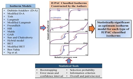
2. Adsorption Isotherm Models
2.1. Dubinin–Astakhov (D–A) Model
2.2. Modified Dubinin–Astakhov (D–A) Model
2.3. Tόth Model
2.4. Langmuir Model
2.5. Modified Langmuir Model
2.6. Freundlich Model
2.7. Hill Model
2.8. Mahle Model
2.9. Brunauer–Emmet–Teller (BET) Model
2.10. Modified BET Model
2.11. Guggenheim–Anderson–De Boer (GAB) Model
2.12. Sun and Chakraborty Model
2.13. Hybrid Model (Henry + Sips)
2.14. Ben Yahia Model
2.15. Universal Isotherm Model
3. Error Evaluation Function
3.1. Root Mean Square Deviation (RMSD)
3.2. Hybrid Fractional Error Deviation (HYBRID)
4. Statistical Tools
4.1. Information-Based Criterion for Model Selection
4.2. Bootstrap Approach
4.3. Bootstrap p-Value and Confidence Interval (CI) of Residual Sum of Squares (RSS)
4.4. Proportion Tests
4.4.1. Chi-Squared Test for Equality of Proportions
4.4.2. Pairwise Test: Multiple Comparisons
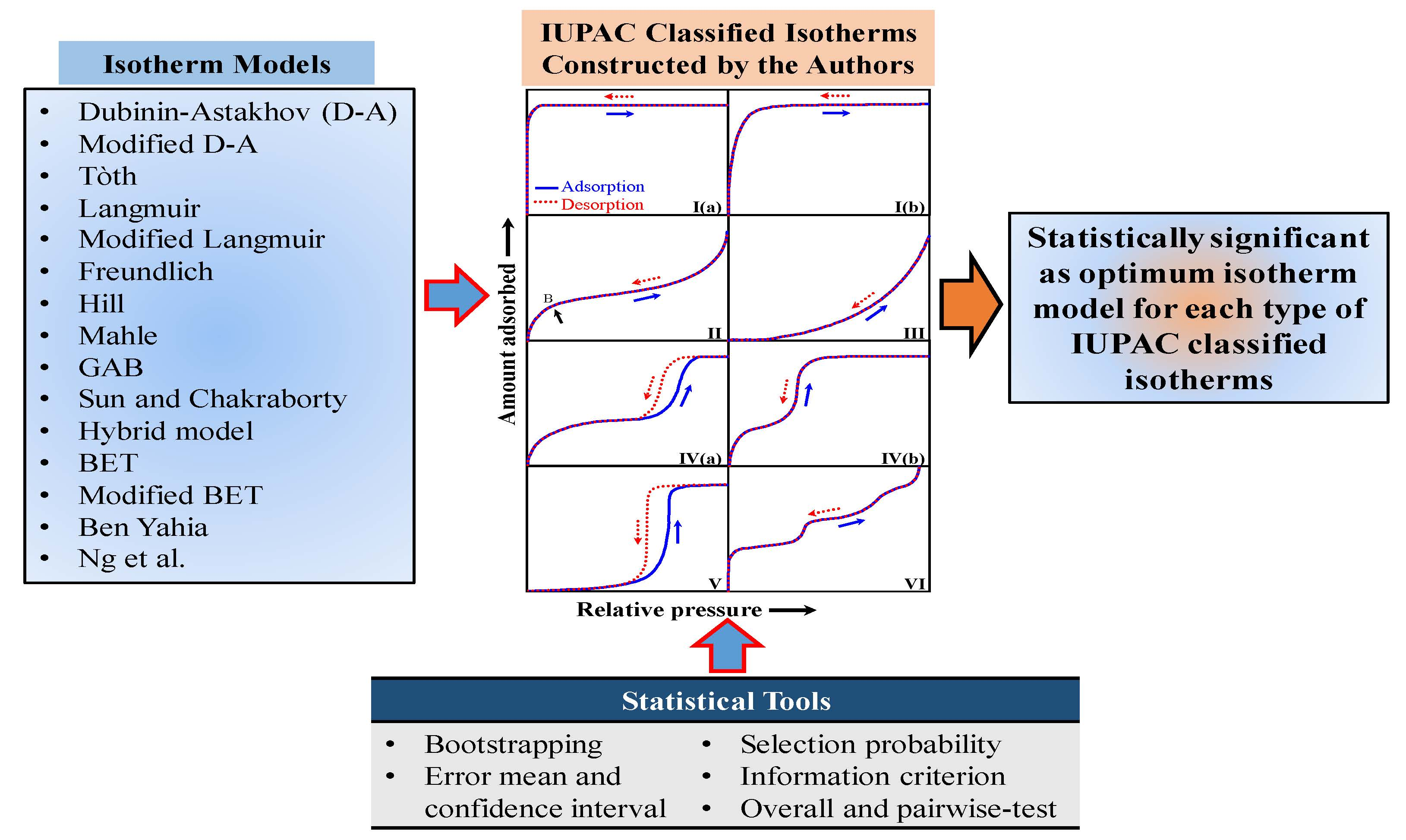
5. Results and Discussion
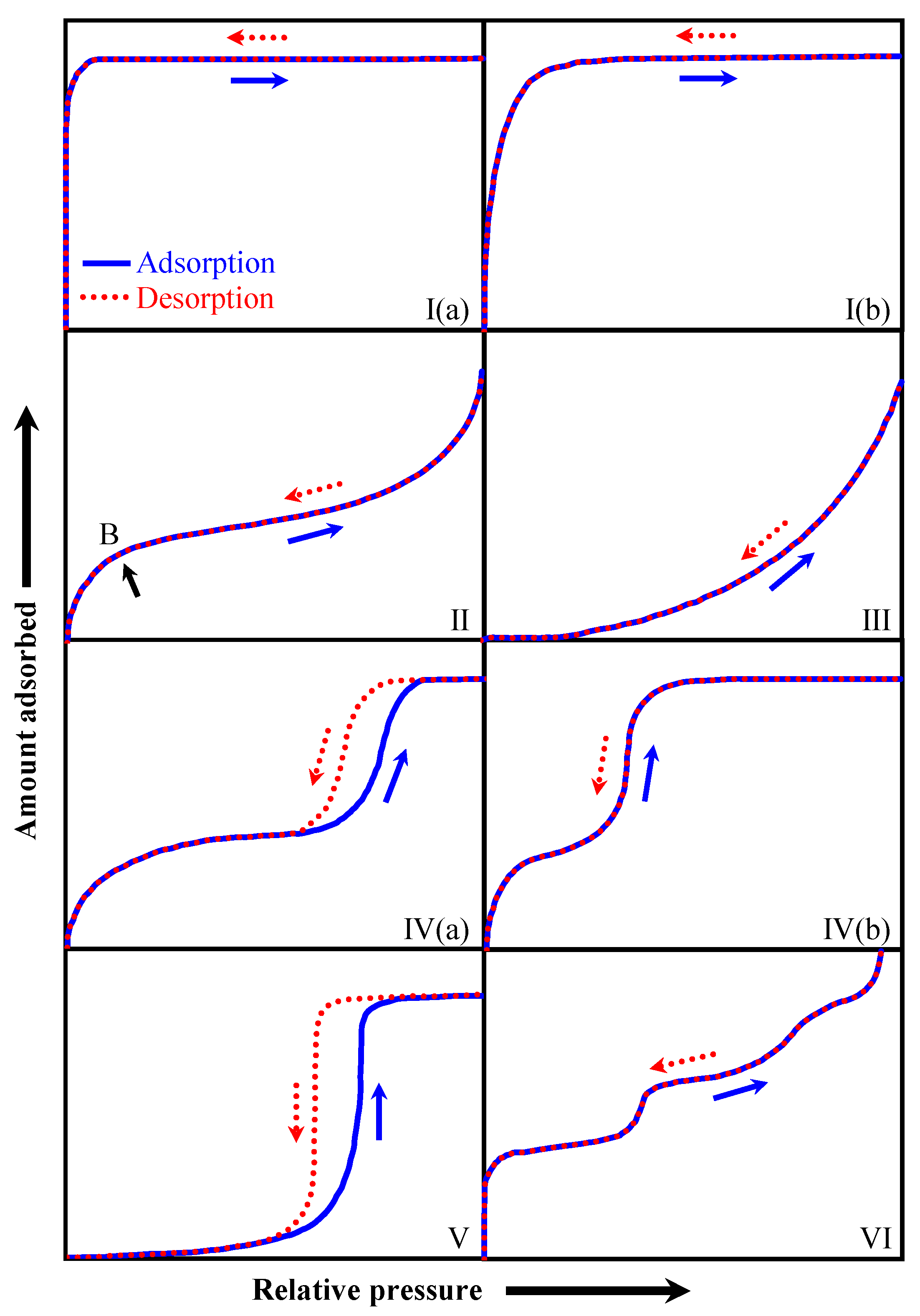
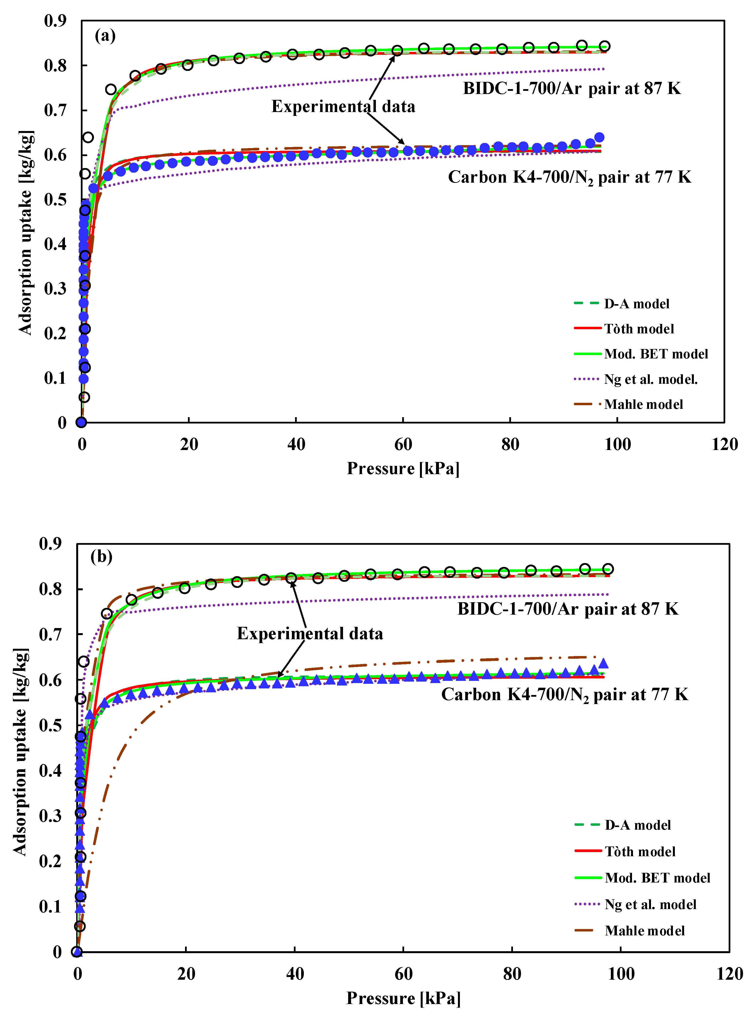
5.1. Type-I(a) Adsorption Isotherm
5.1.1. Bootstrap Error Analysis and Model Selection Using Information Criteria
5.1.2. Overall and Pairwise Proportion Tests
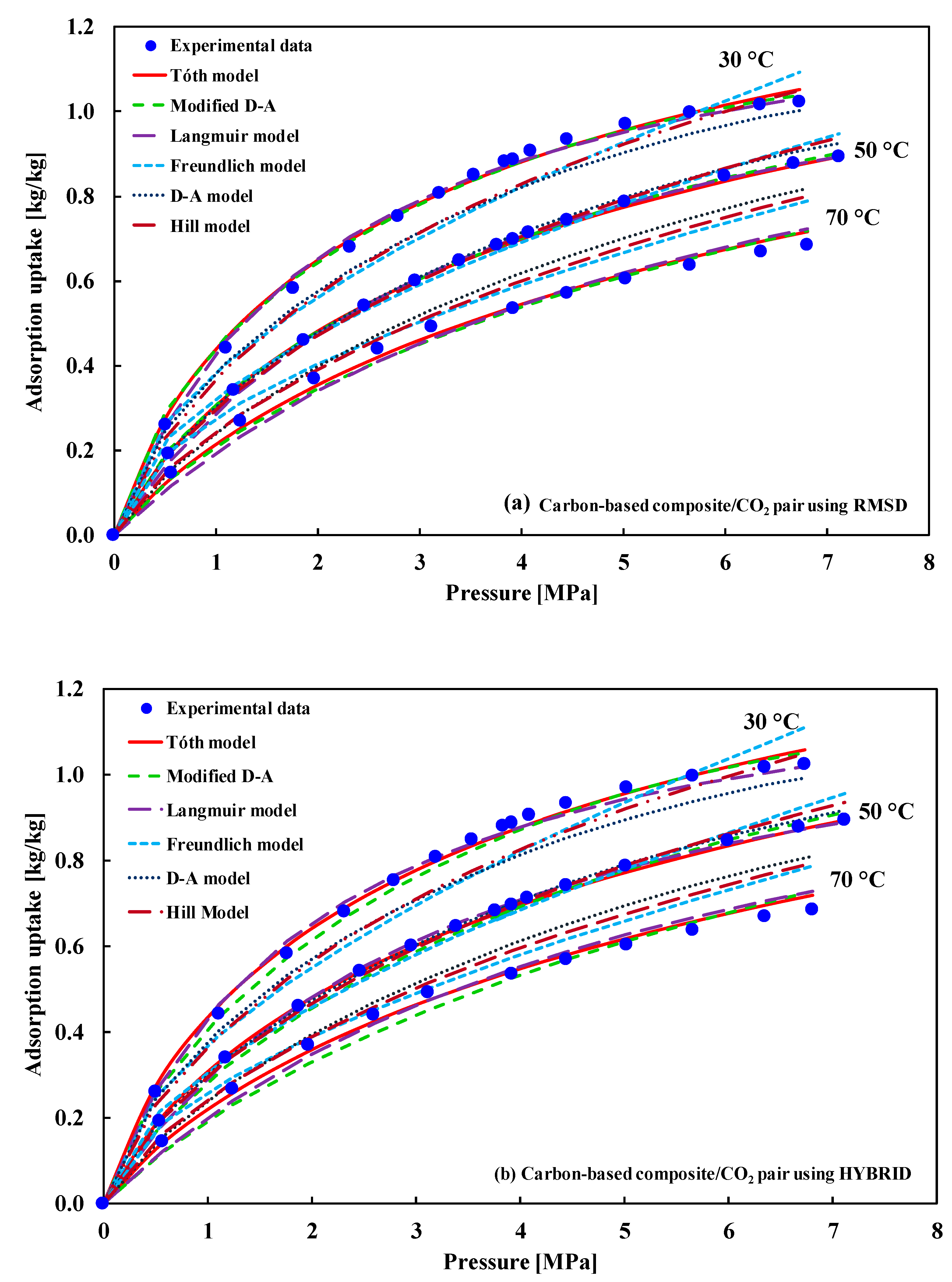
5.2. Type-I(b) Adsorption Isotherm
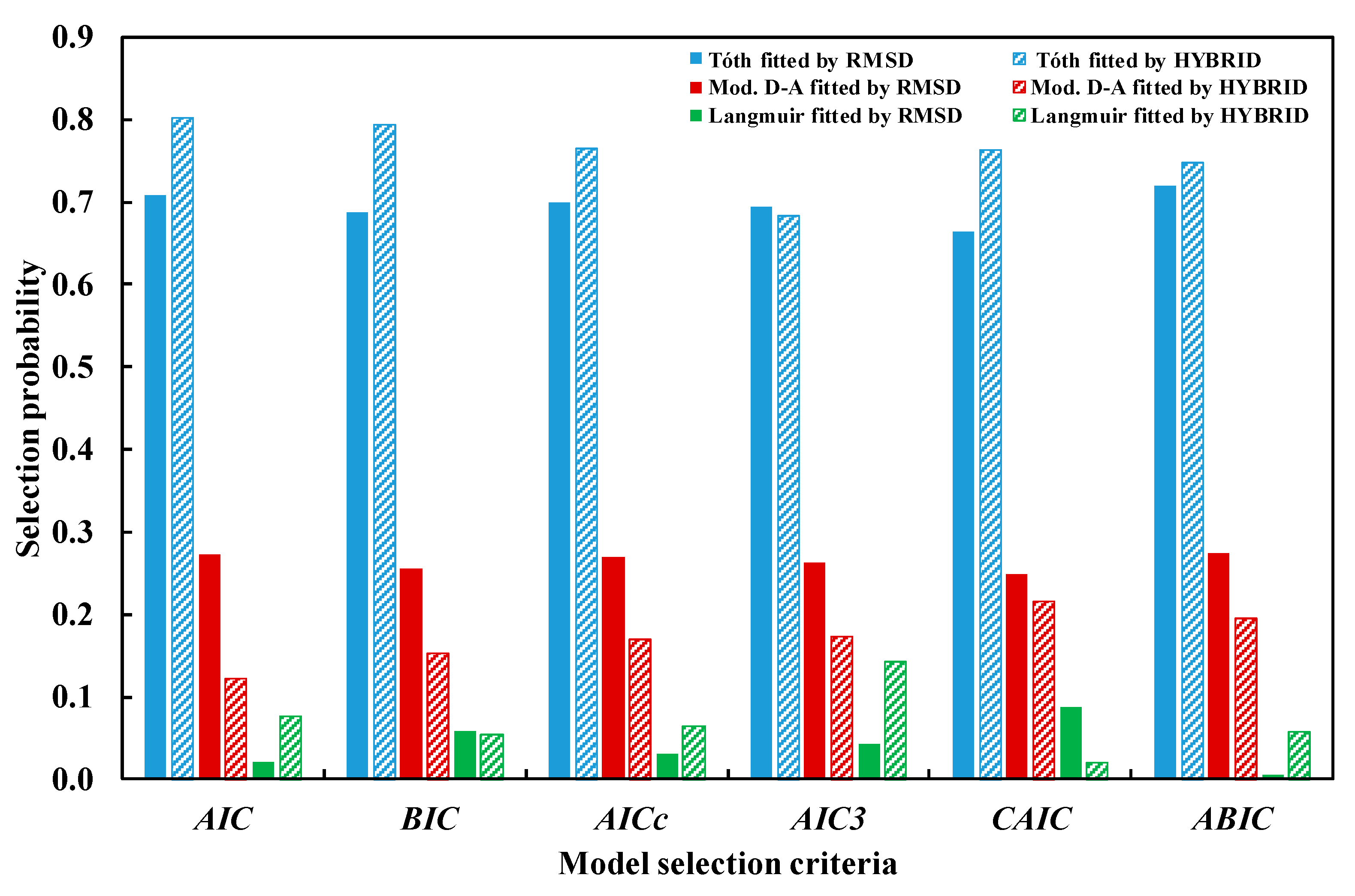
5.2.1. Bootstrap Error Analysis and Model Selection Using Information Criteria
5.2.2. Overall and Pairwise Proportion Tests
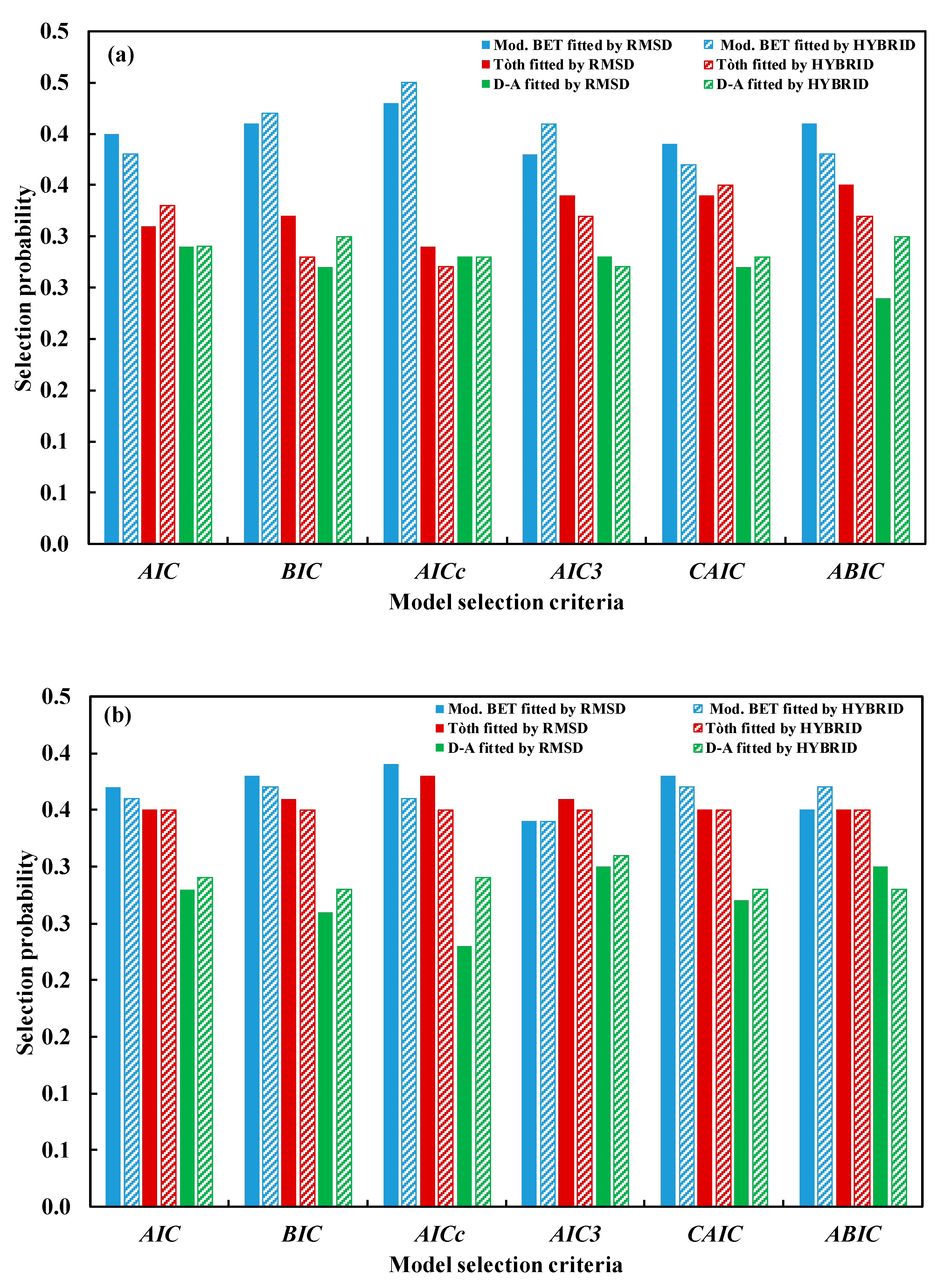
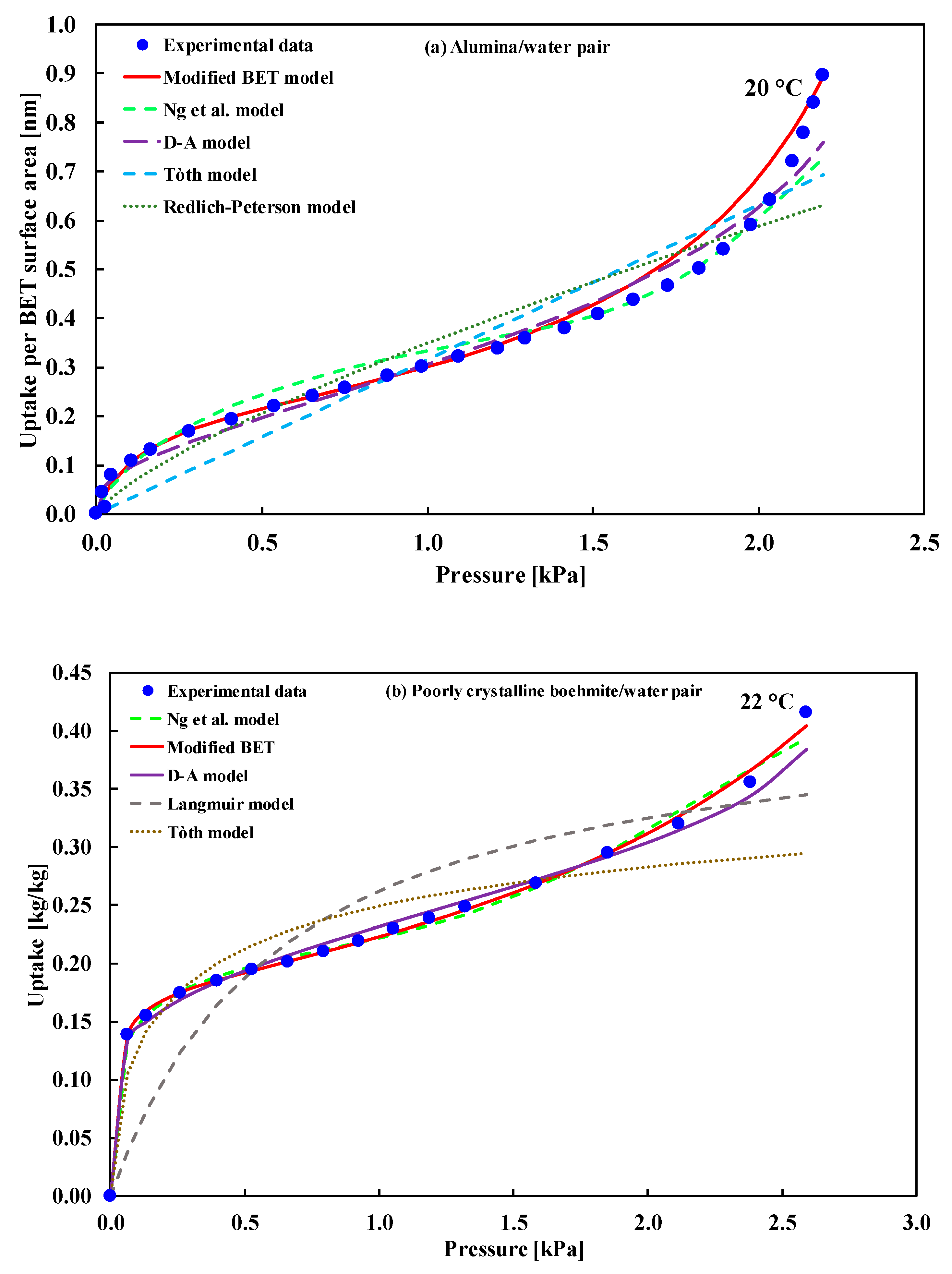
5.3. Type-II Adsorption Isotherm
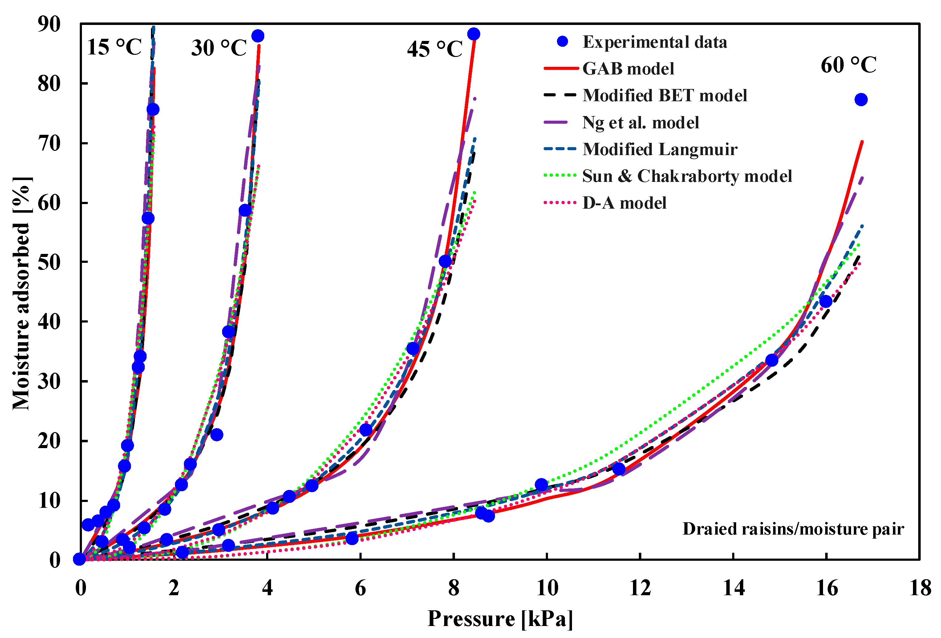
5.4. Type-III Adsorption Isotherm
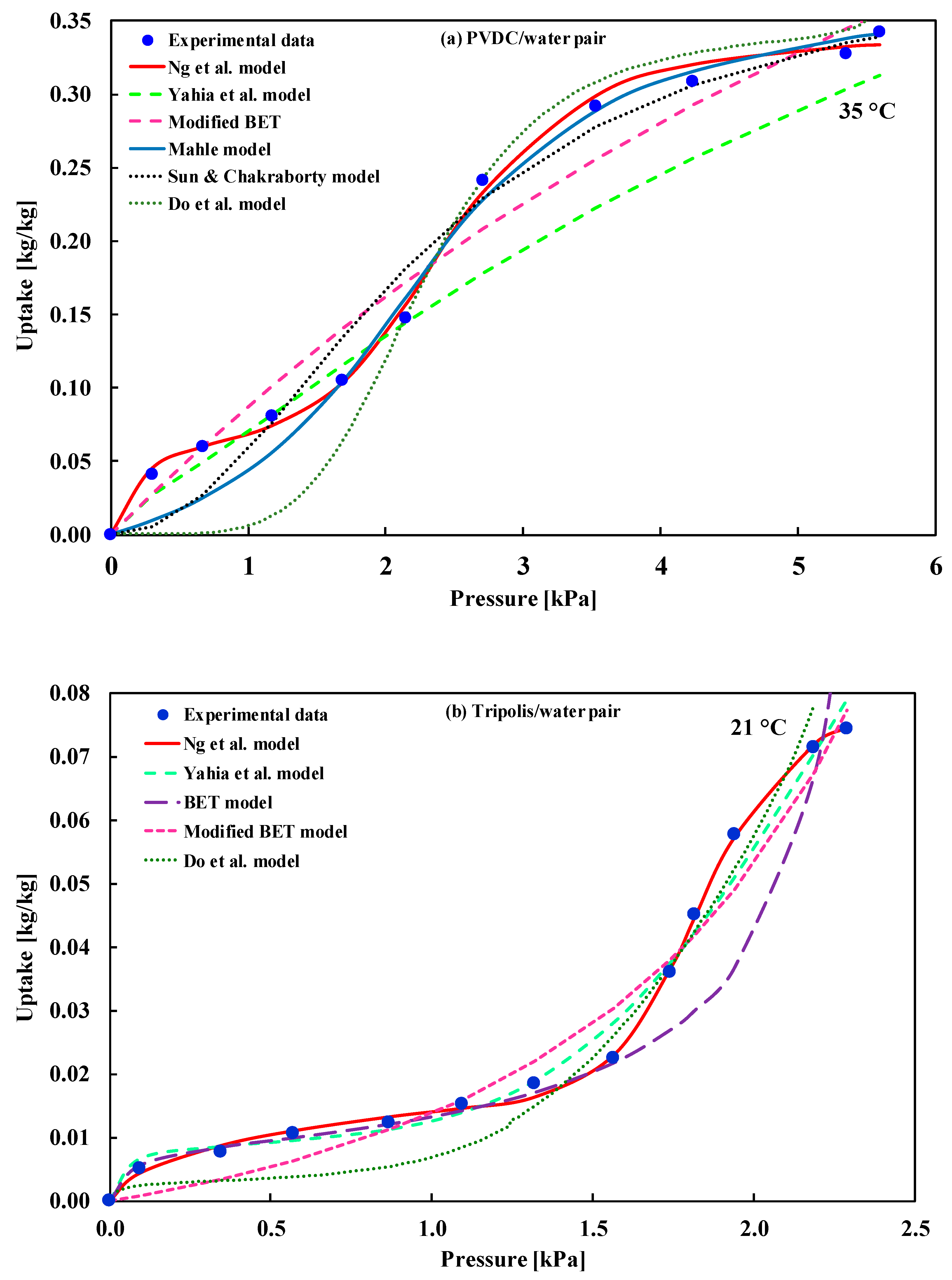
5.5. Type-IV(a) Adsorption Isotherm
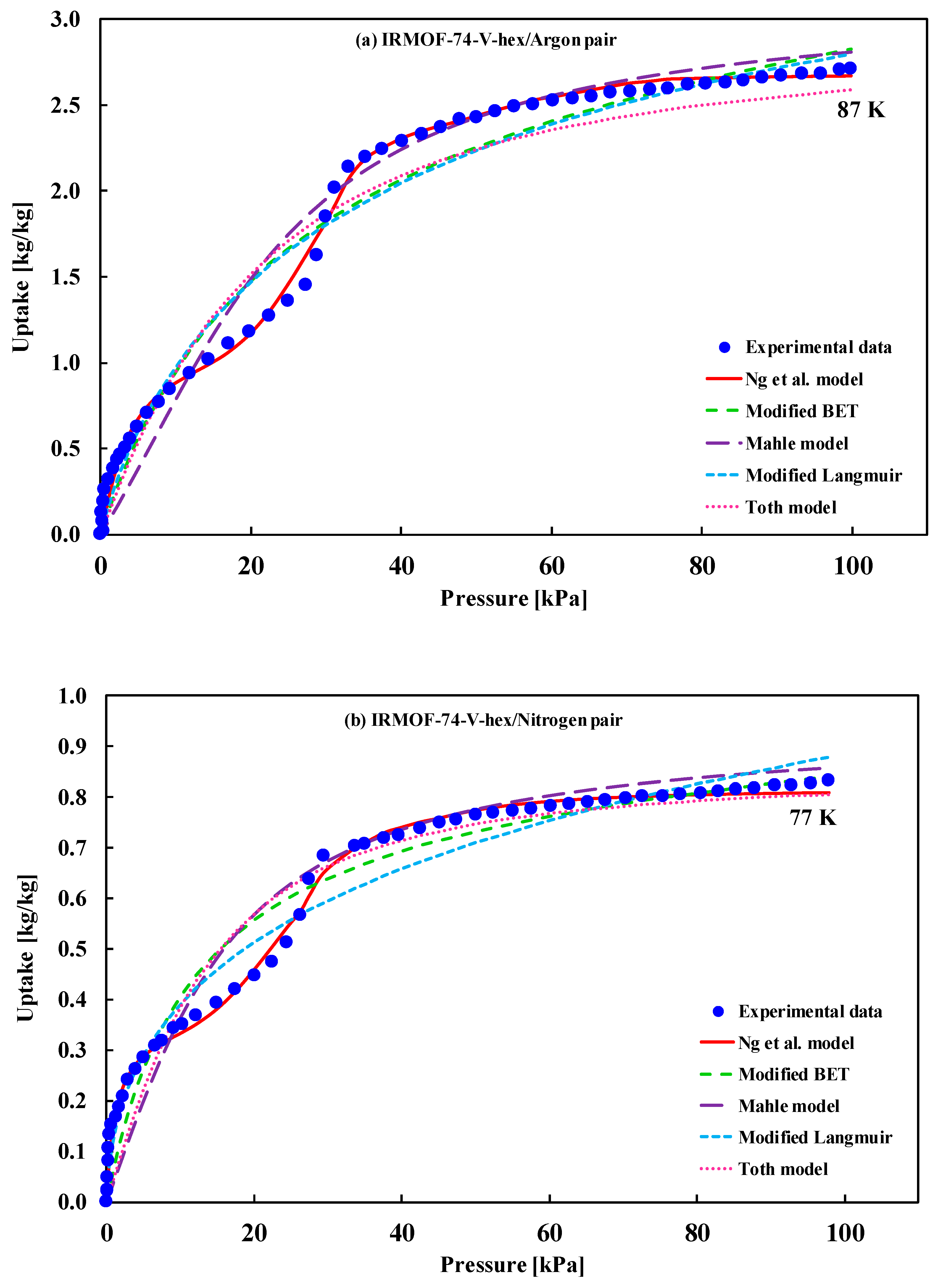
5.6. Type-IV(b) Adsorption Isotherm
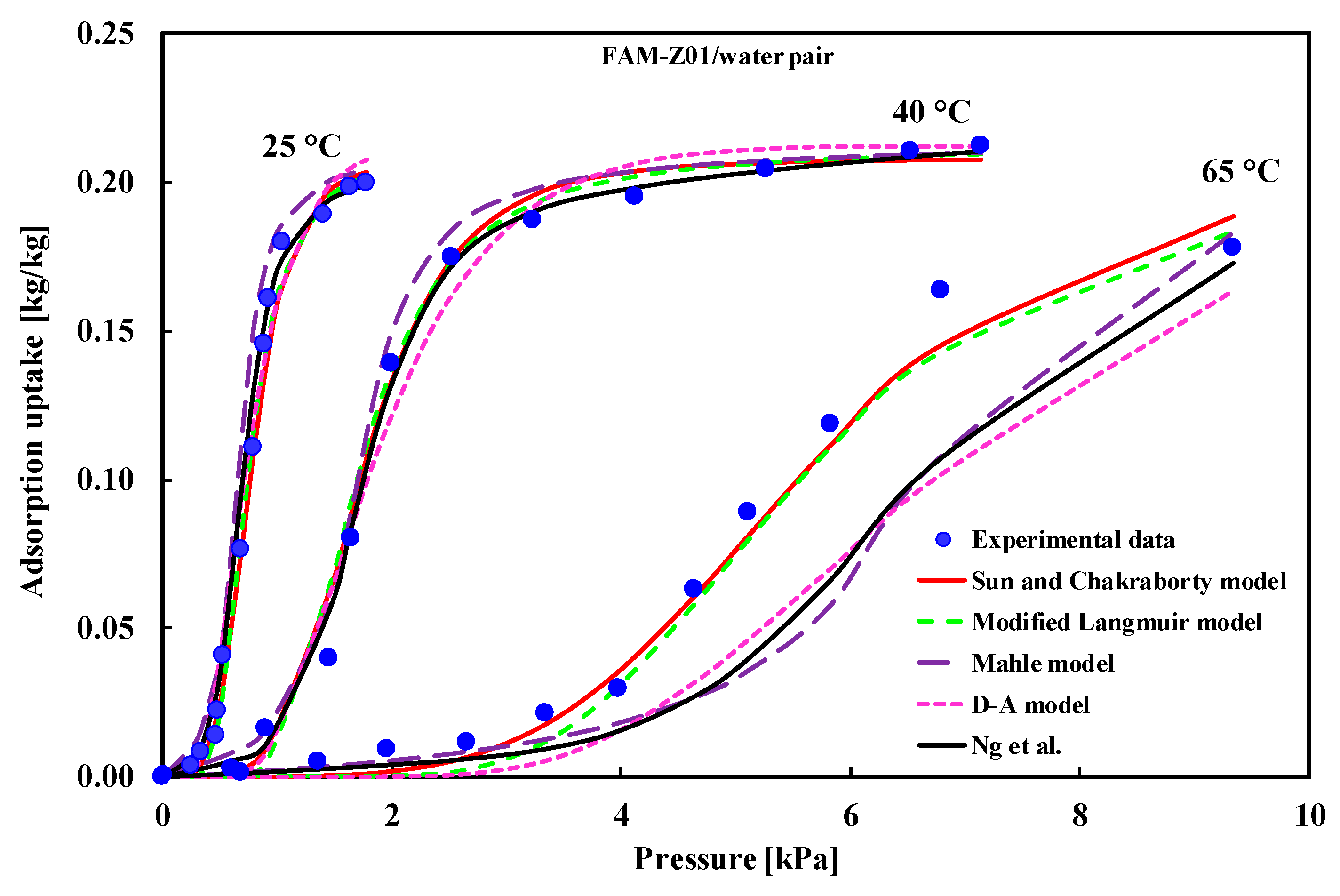
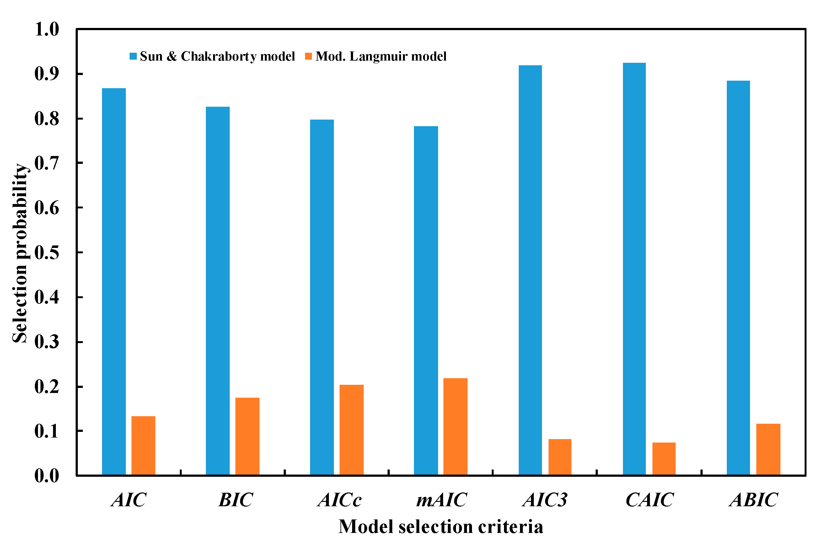
5.7. Type-V Adsorption Isotherm
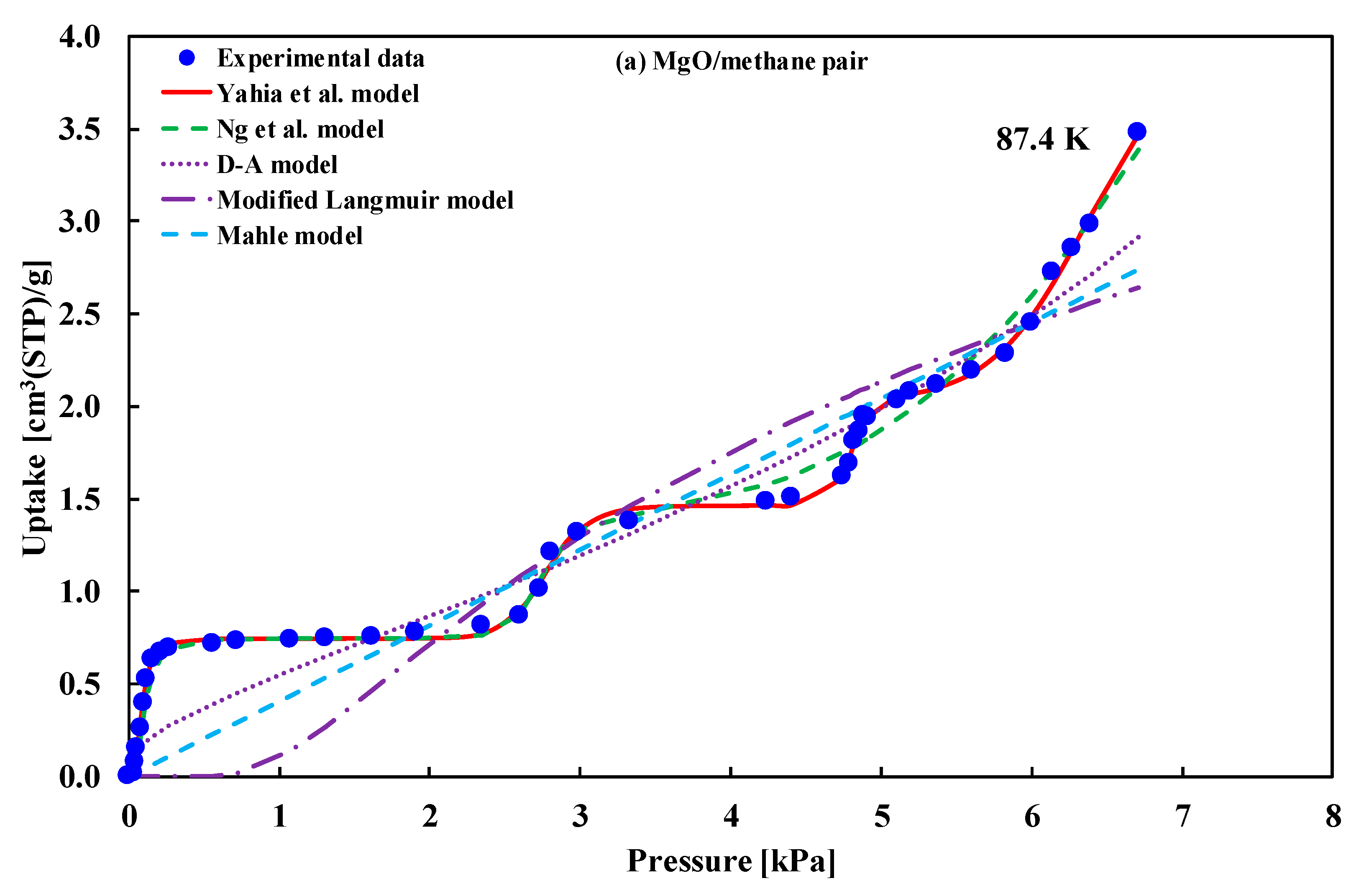
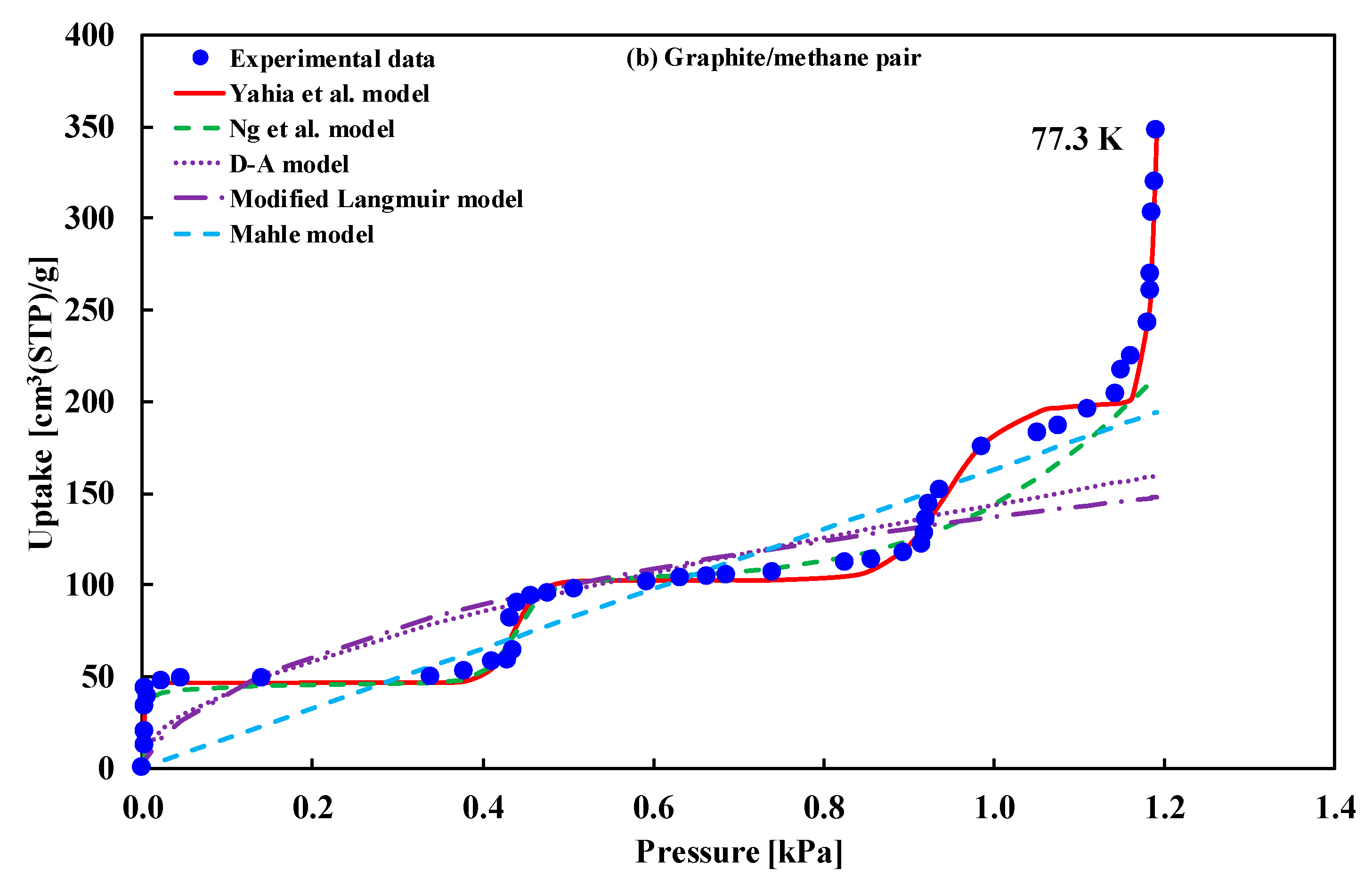
5.8. Type-VI Adsorption Isotherm
6. Conclusions
Author Contributions
Funding
Acknowledgments
Conflicts of Interest
Abbreviations
| ABIC | adjusted bayesian information criterion |
| ACF | activated carbon fiber |
| ACP | activated carbon powder |
| AHT | adsorption heat transformation |
| AIC | akaike information criterion |
| AICc | corrected akaike information criterion |
| BET | brunauer-emmet-teller |
| BIC | bayesian information criterion |
| BIDC | benzimidazole-derived carbons |
| CI | confidence interval |
| D-A | dubinin-astakhov |
| GAB | guggenheim-anderson-de boer |
| GRG | generalized reduced gradient |
| IC | information criterion |
| IRMOF | isoreticular metal-organic framework |
| IUPAC | international union of pure and applied chemistry |
| M-AC | mangrove based activated carbon |
| mAIC | modified akaike information criterion |
| MgO | magnesium oxide |
| PBA | polymer based adsorbent |
| PCB | poorly crystalline boehmite |
| PVDC | polyvinylidene chloride |
| RMSD | root-mean-square deviation |
| RSS | residual sum of squares |
| WPT | waste palm trunk |
References
- Grekova, A.; Gordeeva, L.; Sapienza, A.; Aristov, Y. Adsorption transformation of heat: The applicability in various climatic zones of the Russian federation. Appl. Sci. 2019, 9, 139. [Google Scholar] [CrossRef]
- Saha, B.B.; Koyama, S.; Kashiwagi, T.; Akisawa, A.; Ng, K.C.; Chua, H.T. Waste heat driven dual-mode, multi-stage, multi-bed regenerative adsorption system. Int. J. Refrig. 2003, 26, 749757. [Google Scholar] [CrossRef]
- Palomba, V.; Aprile, M.; Motta, M.; Vasta, S. Study of sorption systems for application on low-emission fishing vessels. Energy 2017, 134, 554–565. [Google Scholar] [CrossRef]
- Ng, K.C.; Thu, K.; Saha, B.B.; Chakraborty, A. Study on a waste heat-driven adsorption cooling cum desalination cycle. Int. J. Refrig. 2012, 35, 685–693. [Google Scholar] [CrossRef]
- Chakraborty, A.; Saha, B.B.; Aristov, Y.I. Dynamic behaviors of adsorption chiller: Effects of the silica gel grain size and layers. Energy 2014, 78, 304–312. [Google Scholar] [CrossRef]
- Pal, A.; Uddin, K.; Thu, K.; Saha, B.B. Activated carbon and graphene nanoplatelets based novel composite for performance enhancement of adsorption cooling cycle. Energy Convers. Manag. 2019, 180, 134–148. [Google Scholar] [CrossRef]
- Chalaev, D.M.; Aristov, Y.I. Assessment of the operation of a low-temperature adsorption refrigerator. Therm. Eng. 2006, 53, 240–244. [Google Scholar] [CrossRef]
- Balaras, C.A.; Grossman, G.; Henning, H.-M.; Ferreira, C.A.I.; Podesser, E.; Wang, L.; Wiemken, E. Solar air conditioning in Europe—An overview. Renew. Sustain. Energy Rev. 2007, 11, 299–314. [Google Scholar] [CrossRef]
- Saha, B.B.; El-Sharkawy, I.I.; Shahzad, M.W.; Thu, K.; Ang, L.; Ng, K.C. Fundamental and application aspects of adsorption cooling and desalination. Appl. Therm. Eng. 2016, 97, 68–76. [Google Scholar] [CrossRef]
- Jaiswal, A.K.; Mitra, S.; Dutta, P.; Srinivasan, K.; Srinivasa Murthy, S. Influence of cycle time and collector area on solar driven adsorption chillers. Sol. Energy 2016, 136, 450–459. [Google Scholar] [CrossRef]
- Solovyeva, M.V.; Gordeeva, L.G.; Aristov, Y.I. “MIL-101(Cr)–methanol” as working pair for adsorption heat transformation cycles: Adsorbent shaping, adsorption equilibrium and dynamics. Energy Convers. Manag. 2019, 182, 299–306. [Google Scholar] [CrossRef]
- Tamainot-Telto, Z.; Metcalf, S.J.; Critoph, R.E.; Zhong, Y.; Thorpe, R. Carbon-ammonia pairs for adsorption refrigeration applications: Ice making, air conditioning and heat pumping. Int. J. Refrig. 2009, 32, 1212–1229. [Google Scholar] [CrossRef]
- Sing, K.S.W. Reporting physisorption data for gas/solid systems with special reference to the determination of surface area and porosity (Recommendations 1984). Pure Appl. Chem. 1985, 57, 603–619. [Google Scholar] [CrossRef]
- Thommes, M.; Kaneko, K.; Neimark, A.V.; Olivier, J.P.; Rodriguez-Reinoso, F.; Rouquerol, J.; Sing, K.S.W. Physisorption of gases, with special reference to the evaluation of surface area and pore size distribution (IUPAC Technical Report). Pure Appl. Chem. 2015, 87, 1051–1069. [Google Scholar] [CrossRef]
- Muttakin, M.; Mitra, S.; Thu, K.; Ito, K.; Saha, B.B. Theoretical framework to evaluate minimum desorption temperature for IUPAC classified adsorption isotherms. Int. J. Heat Mass Transf. 2018, 122, 795–805. [Google Scholar] [CrossRef]
- Ng, K.C.; Burhan, M.; Shahzad, M.W.; Ismail, A. Bin A Universal Isotherm Model to Capture Adsorption Uptake and Energy Distribution of Porous Heterogeneous Surface. Sci. Rep. 2017, 7, 10634. [Google Scholar] [CrossRef]
- Saha, B.B.; Uddin, K.; Pal, A.; Thu, K. Emerging sorption pairs for heat pump applications: An overview. JMST Adv. 2019, 1, 161–180. [Google Scholar] [CrossRef]
- Hu, X.; Radosz, M.; Cychosz, K.A.; Thommes, M. CO2-filling capacity and selectivity of carbon nanopores: Synthesis, texture, and pore-size distribution from quenched-solid density functional theory (QSDFT). Environ. Sci. Technol. 2011, 45, 7068–7074. [Google Scholar] [CrossRef]
- Cychosz, K.A.; Thommes, M. Progress in the Physisorption Characterization of Nanoporous Gas Storage Materials. Engineering 2018, 4, 559–566. [Google Scholar] [CrossRef]
- El-Sharkawy, I.I.; Uddin, K.; Miyazaki, T.; Saha, B.B.; Koyama, S.; Miyawaki, J.; Yoon, S.-H.H. Adsorption of ethanol onto parent and surface treated activated carbon powders. Int. J. Heat Mass Transf. 2014, 73, 445–455. [Google Scholar] [CrossRef]
- Rahman, M.M.; Pal, A.; Uddin, K.; Thu, K.; Saha, B.B. Statistical Analysis of Optimized Isotherm Model for Maxsorb III/Ethanol and Silica Gel/Water Pairs. Evergreen 2018, 5, 1–12. [Google Scholar] [CrossRef]
- Pal, A.; El-Sharkawy, I.I.; Saha, B.B.; Jribi, S.; Miyazaki, T.; Koyama, S. Experimental investigation of CO2 adsorption onto a carbon based consolidated composite adsorbent for adsorption cooling application. Appl. Therm. Eng. 2016, 109, 304–311. [Google Scholar] [CrossRef]
- Pal, A.; Kil, H.S.; Mitra, S.; Thu, K.; Saha, B.B.; Yoon, S.H.; Miyawaki, J.; Miyazaki, T.; Koyama, S. Ethanol adsorption uptake and kinetics onto waste palm trunk and mangrove based activated carbons. Appl. Therm. Eng. 2017, 122, 389–397. [Google Scholar] [CrossRef]
- Pal, A.; Thu, K.; Mitra, S.; El-Sharkawy, I.I.; Saha, B.B.; Kil, H.S.; Yoon, S.H.; Miyawaki, J. Study on biomass derived activated carbons for adsorptive heat pump application. Int. J. Heat Mass Transf. 2017, 110, 7–19. [Google Scholar] [CrossRef]
- Wang, Y.; LeVan, M.D. Adsorption equilibrium of carbon dioxide and water vapor on zeolites 5a and 13X and silica gel: Pure components. J. Chem. Eng. Data 2009, 54, 2839–2844. [Google Scholar] [CrossRef]
- Brancato, V.; Frazzica, A.; Sapienza, A.; Gordeeva, L.; Freni, A. Ethanol adsorption onto carbonaceous and composite adsorbents for adsorptive cooling system. Energy 2015, 84, 177–185. [Google Scholar] [CrossRef]
- Berdenova, B.; Pal, A.; Muttakin, M.; Mitra, S.; Thu, K.; Saha, B.B.; Kaltayev, A. A comprehensive study to evaluate absolute uptake of carbon dioxide adsorption onto composite adsorbent. Int. J. Refrig. 2019, 100, 131–140. [Google Scholar] [CrossRef]
- Pal, A.; Shahrom, M.S.R.; Moniruzzaman, M.; Wilfred, C.D.; Mitra, S.; Thu, K.; Saha, B.B. Ionic liquid as a new binder for activated carbon based consolidated composite adsorbents. Chem. Eng. J. 2017, 326, 980–986. [Google Scholar] [CrossRef]
- Younes, M.M.; El-sharkawy, I.I.; Kabeel, A.E.; Uddin, K.; Pal, A.; Mitra, S.; Thu, K.; Saha, B.B. Synthesis and characterization of silica gel composite with polymer binders for adsorption cooling applications. Int. J. Refrig. 2019, 98, 161–170. [Google Scholar] [CrossRef]
- Sultan, M.; Miyazaki, T.; Koyama, S. Optimization of adsorption isotherm types for desiccant air-conditioning applications. Renew. Energy 2018, 121, 441–450. [Google Scholar] [CrossRef]
- Naono, H.; Hakuman, M. Analysis of adsorption isotherms of water vapor for nonporous and porous adsorbents. J. Colloid Interface Sci. 1991, 145, 405–412. [Google Scholar] [CrossRef]
- Wang, S.L.; Johnston, C.T.; Bish, D.L.; White, J.L.; Hem, S.L. Water-vapor adsorption and surface area measurement of poorly crystalline boehmite. J. Colloid Interface Sci. 2003, 260, 26–35. [Google Scholar] [CrossRef]
- Maroulis, Z.B.; Tsami, E.; Marinos-Kouris, D.; Saravacos, G.D. Application of the GAB model to the moisture sorption isotherms for dried fruits. J. Food Eng. 1988, 7, 63–78. [Google Scholar] [CrossRef]
- Do, D.D.; Do, H.D. Model for water adsorption in activated carbon. Carbon 2000, 38, 767–773. [Google Scholar] [CrossRef]
- Volkova, V.; Kiose, T.; Golubchik, K.; Rakitskaya, T.; Baumer, V. Effect of Both the Phase Composition and Modification Methods on Structural-Adsorption Parameters of Dispersed Silicas. Colloids Interfaces 2018, 3, 1. [Google Scholar]
- Cho, H.S.; Yang, J.; Gong, X.; Zhang, Y.B.; Momma, K.; Weckhuysen, B.M.; Deng, H.; Kang, J.K.; Yaghi, O.M.; Terasaki, O. Isotherms of individual pores by gas adsorption crystallography. Nat. Chem. 2019, 11, 562–570. [Google Scholar] [CrossRef]
- Kayal, S.; Baichuan, S.; Saha, B.B. Adsorption characteristics of AQSOA zeolites and water for adsorption chillers. Int. J. Heat Mass Transf. 2016, 92, 1120–1127. [Google Scholar] [CrossRef]
- Kim, Y.D.; Thu, K.; Ng, K.C. Adsorption characteristics of water vapor on ferroaluminophosphate for desalination cycle. Desalination 2014, 344, 350–356. [Google Scholar] [CrossRef]
- Teo, H.W.B.; Chakraborty, A.; Fan, W. Improved adsorption characteristics data for AQSOA types zeolites and water systems under static and dynamic conditions. Microporous Mesoporous Mater. 2017, 242, 109–117. [Google Scholar]
- Brancato, V.; Frazzica, A. Characterisation and comparative analysis of zeotype water adsorbents for heat transformation applications. Sol. Energy Mater. Sol. Cells 2018, 180, 91–102. [Google Scholar] [CrossRef]
- Yahia, M.B.; Khalfaoui, M.; Hachicha, M.A.; Lamine, A.B.; Torkia, Y.B.; Knani, S. Models for Type VI Adsorption Isotherms from a Statistical Mechanical Formulation. Adsorpt. Sci. Technol. 2013, 31, 341–357. [Google Scholar] [CrossRef]
- Rocky, K.A.; Pal, A.; Moniruzzaman, M.; Saha, B.B. Adsorption characteristics and thermodynamic property fields of polymerized ionic liquid and polyvinyl alcohol based composite/CO2 pairs. J. Mol. Liq. 2019, 294, 111555. [Google Scholar] [CrossRef]
- Astakhov, V.A.; Dubinin, M.M. Development of the concept of volume filling of micropores in the adsorption of gases and vapors by microporous adsorbents-Communication 3. Zeolites with large cavities and a substantial number of adsorption centers. Bull. Acad. Sci. USSR Div. Chem. Sci. 1971, 20, 13–16. [Google Scholar] [CrossRef]
- Do, D.D. Adsorption Analysis: Equilibria and Kinetics: (With CD Containing Computer Matlab Programs); Imperial College Press: London, UK, 1998; Volume 2, ISBN 978-1-78326-224-3. [Google Scholar]
- Amankwah, K.A.G.; Schwarz, J.A. A modified approach for estimating pseudo-vapor pressures in the application of the Dubinin-Astakhov equation. Carbon 1995, 33, 1313–1319. [Google Scholar] [CrossRef]
- Pal, A.; Uddin, K.; Rocky, K.A.; Thu, K.; Saha, B.B. CO2 adsorption onto activated carbon–graphene composite for cooling applications. Int. J. Refrig. 2019, 106, 558–569. [Google Scholar] [CrossRef]
- Ozawa, S.; Kusumi, S.E.I.I.C.H.I.R.O.; Ogino, Y. 1976-OzawaKusumiOgino-Physical adsorption of gases at high pressure. IV. An improvement of the Dubinin—Astakhov adsorption equation. J. Colloid Interface Sci. 1976, 56, 83–91. [Google Scholar] [CrossRef]
- Jribi, S.; Miyazaki, T.; Saha, B.B.; Pal, A.; Younes, M.M.; Koyama, S.; Maalej, A. Equilibrium and kinetics of CO 2 adsorption onto activated carbon. Int. J. Heat Mass Transf. 2017, 108, 1941–1946. [Google Scholar] [CrossRef]
- Liu, Z.; Zhang, Z.; Liu, X.; Wu, T.; Du, X. Supercritical CO2 Exposure-Induced Surface Property, Pore Structure, and Adsorption Capacity Alterations in Various Rank Coals. Energies 2019, 12, 3294. [Google Scholar] [CrossRef]
- Zou, J.; Rezaee, R. A prediction model for methane adsorption capacity in shale gas reservoirs. Energies 2019, 12, 280. [Google Scholar] [CrossRef]
- Wanassi, B.; Hariz, I.B.; Ghimbeu, C.M.; Vaulot, C.; Jeguirim, M. Green carbon composite-derived polymer resin and waste cotton fibers for the removal of alizarin red S dye. Energies 2017, 10, 1321. [Google Scholar] [CrossRef]
- Foo, K.Y.; Hameed, B.H. Insights into the modeling of adsorption isotherm systems. Chem. Eng. J. 2010, 156, 2–10. [Google Scholar] [CrossRef]
- Mahle, J.J. An adsorption equilibrium model for Type 5 isotherms. Carbon 2002, 40, 2753–2759. [Google Scholar] [CrossRef]
- Sun, B.; Chakraborty, A. Thermodynamic formalism of water uptakes on solid porous adsorbents for adsorption cooling applications. Appl. Phys. Lett. 2014, 104, 201901. [Google Scholar] [CrossRef]
- Hogg, R.V.; Tanis, E.A.; Zimmerman, D.L. Probability and Statistical Interference; Pearson Education, Inc.: Fort Worth, TX, USA, 2003; ISBN 9780133936544. [Google Scholar]
- Porter, J.F.; McKay, G.; Choy, K.H. The prediction of sorption from a binary mixture of acidic dyes using single- and mixed-isotherm variants of the ideal adsorbed solute theory. Chem. Eng. Sci. 1999, 54, 5863–5885. [Google Scholar] [CrossRef]
- Sclove, L.S. Application of model selection criteria to some problems in multivariate analysis. Psychometrika 1987, 52, 333–343. [Google Scholar] [CrossRef]
- Koukouvinos, C.; Mylona, K.; Skountzou, A. A variable selection method for analyzing supersaturated designs. Commun. Stat. Simul. Comput. 2011, 40, 484–496. [Google Scholar] [CrossRef][Green Version]
- Dziak, J.J.; Coffman, D.L.; Lanza, S.T.; Li, R. Sensitivity and Specificity of Information Criteria. Peer J. Prepr. 2015, 1–20. [Google Scholar] [CrossRef]
- Akaike, H. Fitting Autoregressive Models for Prediction. Ann. Inst. Stat. Math. 1969, 21, 243–247. [Google Scholar] [CrossRef]
- Bozdogan, H. Model selection and Akaike’s Information Criterion (AIC): The general theory and its analytical extensions. Psychometrika 1987, 52, 345–370. [Google Scholar] [CrossRef]
- Kamruzzaman, M.; Khudri, M.M.; Rahman, M.M. Modeling and Predicting Stock Market Returns: A Case Study on Dhaka Stock Exchange of Bangladesh. Dhaka Univ. J. Sci. 2017, 65, 97–101. [Google Scholar]
- Kullback, S.; Leibler, R.A. On Information and Sufficiency. Ann. Math. Stat. 2010, 22, 79–86. Available online: http://www.jstor (accessed on 15 November 2019). [CrossRef]
- Hurvich, C.M.; Tsai, C.-L. Regression and Time Series Model Selection in Small Samples. Biometrika 1989, 76, 297–307. [Google Scholar] [CrossRef]
- Sugiura, N. Further analysts of the data by akaike’ s information criterion and the finite corrections. Commun. Stat. Theory Methods 1978, 7, 13–26. [Google Scholar] [CrossRef]
- Burnham, K.P.; Anderson, D.R. Multimodel Inference. Sociol. Methods Res. 2004, 33, 261–304. [Google Scholar] [CrossRef]
- Anderson, D.B.K. Model Selection and Multimodel Inference; Springer: New York, NY, USA, 2002; p. 515. [Google Scholar]
- Phoa, F.K.H.; Pan, Y.H.; Xu, H. Analysis of supersaturated designs via the Dantzig selector. J. Stat. Plan. Inference 2009, 139, 2362–2372. [Google Scholar] [CrossRef]
- Schwarz, G. Estimating the Dimension of a Model. Ann. Stat. 1978, 6, 461–464. [Google Scholar] [CrossRef]
- Rissanen, J. Modeling by shortest data description. Automatica 1978, 14, 465–471. [Google Scholar] [CrossRef]
- Boekee, D.E.; Buss, H.H. Order estimation of autoregressive models. In Proceedings of the 4th Aachen Colloquium: Theory and Application of Signal Processing, Aachen, Germany, 1981; pp. 126–130. [Google Scholar]
- Efron, B.; Tibshirani, R.J. Introduction to the Bootstrap; Springer: Toronto, ON, Canada, 1993; ISBN 9780412042317. [Google Scholar]
- Joshi, M.; Kremling, A.; Seidel-Morgenstern, A. Model based statistical analysis of adsorption equilibrium data. Chem. Eng. Sci. 2006, 61, 7805–7818. [Google Scholar] [CrossRef]
- Saha, S.K.; Haque, M.E.; Islam, D.; Rahman, M.M.; Islam, M.R.; Parvin, A.; Rahman, S. Comparative study between the effect of Momordica charantia (wild and hybrid variety) on hypoglycemic and hypolipidemic activity of alloxan induced type 2 diabetic long-evans rats. J. Diabetes Mellit. 2012, 2, 133–137. [Google Scholar] [CrossRef]
- Gay, J.M.; Suzanne, J. Wetting, surface melting, and freezing of thin films of methane adsorbed on MgO(100). Am. Phys. Soc. 1990, 41, 346–351. [Google Scholar] [CrossRef]
- Bienfait, M.; Zeppenfeld, P.; Gay, J.M.; Palmari, J.P. Surface melting on the close-packed (111) face of methane thin films condensed on graphite. Surf. Sci. 1990, 226, 327–338. [Google Scholar] [CrossRef]


| Adsorption Pair | Type | Best Fitted Model | Reference |
|---|---|---|---|
| (i) Carbon K4-700/N2 at 77 K (ii) BIDC-1-700/Ar at 87 K (pore size less than 1 nm for both (i) and (ii)). | Type-I(a) | Fitted model is not available | (i) Hu et al. [18] (ii) Cychosz et al. [19] |
| (i) Maxsorb III/ethanol (ii) Silica gel/water (iii) Carbon based composite/CO2 (iv) Carbon based composite/CO2 (v) WPT-AC/ethanol (vi) M-AC/ethanol (vii) Zeolite/water at 25 °C (viii) (SRD 1352/3, FR 20, ATO and AP4-60/COCL-1200)/ N2 * (ix) Ionic liquid binder based composite/ethanol (x) Silica gel based composite/water | Type-I(b) | (i) D–A model (ii) Tόth (iii) Tόth (iv) D–A and Tόth (v) D–A and Tόth (vi) D–A and Tόth (vii) Tόth (viii) D–A (ix) D–A (x) Tόth | (i) El-Sharkawy et al. [20] (ii) Rahman et al. [21] (iii) Pal et al. [22] (iv) Berdenova et al. [23] (v) Pal et al. [24,25] (vi) Pal et al. [24,25] (vii) Wang et al. [26] (viii) Brancato et al. [27] (ix) Pal et al. [28] (x) Younes et al. [29] |
| (i) PBA/water at 25 °C (ii) Alumina/water at 20 °C (iii) PCB/water at 22 °C | Type-II | (i) GAB model (ii) BET model (iii) Not fitted | (i) Sultan et al. [30] (ii) Naono et al. [31] (iii) Wang et al. [32] |
| (i) ACP/water at 30 °C (ii) Dried fruits/moisture | Type-III | (i) D–A model (ii) GAB model | (i) Sultan et al. [30] (ii) Maroulis et al. [33] |
| (i) Oxidized carbon/water (ii) PVDC/water at 35 °C iii) Tripolis/water at 21 °C | Type-IV(a) | (i) Do et al. model (ii) Do et al. model (iii) BET model | (i) Do et al. [34] (ii) Do et al. [34] (iii) Rakitskaya et al. [35] |
| (i) IRMOF-74-V-hex/argon at 87 K (ii) IRMOF-74-V-hex/nitrogen at 77 K (pore size less than 4 nm) | Type-IV(b) | The fitted model is not available | (i) Cho et al. [36] (ii) Cho et al. [36] |
| (i) ACF/water at 30 °C (ii) Hydrophobic carbon/water (iii) AQSOA-Z01/water and AQSOA-Z02/water (iv) Ferroaluminophosphate/water (v) AQSOA zeolite/ water (vi) AlPO-18, FAPO-34, SAPO-34/water | Type-V | (i) D–A model (ii) Do et al. model (iii) D–A, modified Langmuir (iv) Hybrid model (v) D–A, modified Langmuir, Sun and Chakraborty (vi) D–A model | (i) Sultan et al. [30] (ii) Do et al. [34] (iii) Kayal et al. [37] (iv) Kim et al. [38] (v) Teo et al. [39] (vi) Brancato et al. [40] |
| (i) MgO (100)/methane (ii) Exfoliated graphite/methane | Type-VI | (i) Ng et al. model (ii) Yahia et al. model | (i) Ng et al. [16] (ii) Yahia et al. [41] |
| Model | Mean RMSD | CI of RMSD | Mean HYBRID | CI of HYBRID |
|---|---|---|---|---|
| K4-700/N2 pair | ||||
| Tόth | 0.0745 | (0.045, 0.0956) | 1.884 | (1.24, 2.152) |
| D–A | 0.0838 | (0.047, 0.0971) | 1.912 | (1.55, 2.923) |
| Mod. BET | 0.0638 | (0.050, 0.0723) | 1.871 | (1.52, 1.983) |
| Ng et al. | 0.1066 | (0.032, 0.3254) | 1.913 | (1.43, 3.851) |
| Mahle | 0.1019 | (0.042, 0.2321) | 4.146 | (3.654, 5.123) |
| BIDC-1-700/Ar pair | ||||
| Tόth | 0.1047 | (0.045, 0.126) | 3.6648 | (2.24, 4.152) |
| D–A | 0.0936 | (0.047, 0.0971) | 8.9234 | (6.55, 10.923) |
| Mod. BET | 0.0872 | (0.050, 0.0986) | 3.5624 | (2.52, 4.783) |
| Ng et al. | 0.1245 | (0.032, 0.3254) | 12.354 | (8.43, 15.851) |
| Mahle | 0.1154 | (0.042, 0.2921) | 4.8132 | (2.65, 7.123) |
| Model | Error Mean | AIC | BIC | AICc | mAIC | AIC3 | CAIC | ABIC |
|---|---|---|---|---|---|---|---|---|
| K4-700/N2 pair | ||||||||
| Using RMSD error mean | ||||||||
| Tόth | 0.0745 | -223.16 | −214.78 | −222.43 | −199.16 | −219.16 | −210.78 | −227.36 |
| D–A | 0.0838 | −218.08 | −211.79 | −217.65 | −206.08 | −215.08 | −208.79 | −221.23 |
| Mod. BET | 0.0638 | −234.48 | −228.20 | −234.06 | −222.48 | −231.48 | −225.20 | −237.64 |
| Ng et al. | 0.1066 | −195.68 | −181.02 | −193.53 | −111.68 | −188.68 | −174.02 | −203.04 |
| Mahle | 0.1019 | −204.38 | −196.00 | −203.65 | −180.38 | −200.38 | −192.00 | −208.58 |
| Using HYBRID error mean | ||||||||
| Tόth | 1.884 | −29.33 | −20.96 | −28.61 | −5.33 | −25.33 | −16.96 | −33.54 |
| D–A | 1.912 | −30.47 | −24.19 | −30.05 | −18.47 | −27.47 | −21.19 | −33.63 |
| Mod. BET | 1.871 | −31.78 | −25.49 | −31.35 | −19.78 | −28.78 | −22.49 | −34.93 |
| Ng et al. | 1.913 | −22.44 | −7.78 | −20.29 | 61.56 | −15.44 | −0.78 | −29.80 |
| Mahle | 4.146 | 17.96 | 26.34 | 18.69 | 41.96 | 21.96 | 30.34 | 13.76 |
| BIDC-1-700/Ar pair | ||||||||
| Using RMSD error mean | ||||||||
| Tόth | 0.1047 | −69.02 | −63.69 | −67.28 | −45.02 | −65.02 | −59.69 | −76.12 |
| D–A | 0.0936 | −74.15 | −70.16 | −73.15 | −62.15 | −71.15 | −67.16 | −79.48 |
| Mod. BET | 0.0872 | −76.14 | −72.14 | −75.14 | −64.14 | −73.14 | −69.14 | −81.47 |
| Ng et al. | 0.1245 | −58.17 | −48.84 | −52.57 | 25.83 | −51.17 | −41.84 | −70.60 |
| Mahle | 0.1154 | −66.29 | −60.96 | −64.55 | −42.29 | −62.29 | −56.96 | −73.40 |
| Using HYBRID error mean | ||||||||
| Tόth | 3.6648 | 30.54 | 35.86 | 32.27 | 54.54 | 34.54 | 39.86 | 23.43 |
| D–A | 8.9234 | 53.45 | 57.45 | 54.45 | 65.45 | 56.45 | 60.45 | 48.12 |
| Mod. BET | 3.5624 | 27.74 | 31.74 | 28.74 | 39.74 | 30.74 | 34.74 | 22.41 |
| Ng et al. | 12.354 | 70.56 | 79.89 | 76.16 | 154.56 | 77.56 | 86.89 | 58.12 |
| Mahle | 4.8132 | 38.17 | 43.50 | 39.91 | 62.17 | 42.17 | 47.50 | 31.06 |
| Test | AIC | BIC | AICc | mAIC | AIC3 | CAIC | ABIC |
|---|---|---|---|---|---|---|---|
| Carbon K4-700/N2 | |||||||
| Overall | 2.0 × 10⁻¹⁵ (2.3 × 10⁻¹⁴) | 2.1 × 10− (2.1 × 10⁻¹³) | 2.2 × 10⁻¹⁵ (2.0 × 10⁻¹⁴) | 2.0 × 10⁻¹³ (2.2 × 10⁻¹²) | 2.1 × 10⁻¹⁵ (2.2 × 10⁻¹³) | 2.0 × 10⁻¹⁴ (2.2 × 10⁻¹⁴) | 2.1 × 10⁻¹⁵ (2.2 × 10⁻¹³) |
| Mod. BET vs. Tόth | 2.0 × 10⁻⁴ (2.1 × 10⁻⁵) | 2.1 × 10⁻⁵ (2.0 × 10⁻⁴) | 2.2 × 10⁻³ (2.1 × 10⁻⁴) | 1.4 × 10− (1.2 × 10⁻³) | 1.8 × 10⁻⁴ (2.1 × 10⁻³) | 1.9 × 10⁻³ (2.1 × 10⁻³) | 2.1 × 10⁻⁴ (2.2 × 10⁻³) |
| Mod. BET vs. D–A | 1.5 × 10⁻⁸ (1.9 × 10⁻⁸) | 2.1 × 10⁻⁹ (2.0 × 10⁻⁷) | 1.1 × 10⁻⁸ (2.1 × 10⁻⁸) | 2.0 × 10⁻⁷ (2.0 × 10⁻⁷) | 2.0 × 10⁻⁸ (1.9 × 10⁻⁷) | 1.7 × 10⁻⁹ (2.2 × 10⁻⁹) | 2.1 × 10⁻¹¹ (1.9 × 10⁻¹²) |
| BIDC-1-700/Ar pair | |||||||
| Overall | 2.0 × 10⁻⁴ (2.3 × 10⁻³) | 2.2 × 10⁻³ (2.1 × 10⁻³) | 2.1 × 10⁻⁴ (2.3 × 10⁻³) | 2.4 × 10⁻³ (2.1 × 10⁻⁴) | 2.1 × 10⁻⁴ (2.3 × 10⁻⁵) | 2.5 × 10⁻³ (2.1 × 10⁻⁴) | 2.2 × 10⁻⁴ (2.3 × 10⁻³) |
| Mod. BET vs. Tόth | 0.0235 (0.0351) | 0.0351 (0.0421) | 0.2363 (0.5324) | 0.0425 (0.0354) | 0.0573 (0.0784) | 0.2381 (0.1465) | 0.0715 (0.0471) |
| Mod. BET vs. D–A | 1.6× 10⁻³ (1.7× 10⁻⁴) | 1.1 × 10⁻⁴ (2.4 × 10⁻³) | 1.5 × 10⁻³ (2.3 × 10⁻³) | 1.4 × 10⁻⁴ (2.2 × 10⁻³) | 2.2 × 10⁻³ (1.5 × 10⁻⁴) | 1.9 × 10⁻⁴ (2.1 × 10⁻³) | 2.2 × 10⁻³ (1.44) |
| Model | Mean RMSD | CI of RMSD | Mean HYBRID | CI of HYBRID |
|---|---|---|---|---|
| D–A | 0.05624 | (0.0457, 0.0650) | 0.4893 | (0.3432, 0.6382) |
| Mod. D–A | 0.01532 | (0.0125, 0.0179) | 0.1096 | (0.0745, 0.1438) |
| Tόth | 0.01435 | (0.0122, 0.0165) | 0.0373 | (0.0276, 0.0473) |
| Freundlich | 0.05178 | (0.0451, 0.0583) | 0.4353 | (0.3282, 0.5444) |
| Langmuir | 0.01839 | (0.0157, 0.0209) | 0.0724 | (0.0516, 0.0960) |
| Hill | 0.04871 | (0.0451, 0.0583) | 0.3816 | (0.2740, 0.4965) |
| Model | Error Mean | AIC | BIC | AICc | mAIC | AIC3 | CAIC | ABIC |
|---|---|---|---|---|---|---|---|---|
| Using HYBRID error mean | ||||||||
| D–A | 0.4893 | −56.61 | −51.70 | −55.90 | −44.61 | −53.61 | −48.70 | −61.08 |
| Mod. D–A | 0.1096 | −114.43 | −107.88 | −113.22 | −90.43 | −110.43 | −103.88 | −120.38 |
| Tόth | 0.0373 | −157.53 | −150.98 | −156.32 | −133.53 | −153.53 | −146.98 | −163.49 |
| Freundlich | 0.4353 | −63.29 | −60.01 | −62.95 | −59.29 | −61.29 | −58.01 | −66.27 |
| Langmuir | 0.0724 | −133.03 | −128.11 | −132.32 | −121.03 | −130.03 | −125.11 | −137.50 |
| Hill | 0.3815 | −66.56 | −61.65 | −65.85 | −54.56 | −63.56 | −58.65 | −71.03 |
| Using RMSD error mean | ||||||||
| D–A | 0.0562 | −143.15 | −138.24 | −142.44 | −131.15 | −140.15 | −135.24 | −147.62 |
| Mod. D–A | 0.0153 | −193.17 | −186.62 | −191.96 | −169.17 | −189.17 | −182.62 | −199.12 |
| Tóth | 0.0143 | −195.78 | −189.23 | −194.57 | −171.78 | −191.78 | −185.23 | −201.74 |
| Freundlich | 0.0517 | −148.45 | −145.18 | −148.11 | −144.45 | −146.45 | −143.18 | −151.43 |
| Langmuir | 0.0183 | −187.86 | −182.95 | −187.16 | −175.86 | −184.86 | −179.95 | −192.33 |
| Hill | 0.0487 | −148.90 | −143.99 | −148.19 | −136.90 | −145.90 | −140.99 | −153.37 |
| Test | AIC | BIC | AICc | mAIC | AIC3 | CAIC | ABIC |
|---|---|---|---|---|---|---|---|
| Overall | 2.1 × 10⁻¹⁶ (2.2 × 10⁻¹²) | 2.1 × 10⁻¹⁵ (2.2 × 10⁻¹³) | 2.1 × 10⁻¹⁶ (2.2 × 10⁻¹⁴) | 2.2 × 10⁻¹⁴ (2.2 × 10⁻¹³) | 2.2 × 10⁻¹⁶ (2.2 × 10⁻¹⁴) | 2.0 × 10⁻¹³ (2.2 × 10⁻¹⁶) | 2.2 × 10⁻¹⁶ (2.2 × 10⁻¹⁵) |
| Tόth vs. Mod. D–A | 2.0 × 10⁻¹² (2.0 × 10⁻¹⁶) | 2.0 × 10⁻¹¹ (2.0 × 10⁻¹⁶) | 2.0 × 10⁻¹¹ (2.0 × 10⁻¹⁶) | 1.0 × 10⁻¹⁰ (1.0 × 10⁻¹⁰) | 2.0 × 10⁻¹³ (2.0 × 10⁻¹⁶) | 2.1 × 10⁻¹² (2.0 × 10⁻¹⁶) | 2.0 × 10⁻¹³ (2.0 × 10⁻¹⁶) |
| Mod.D–A vs. Langmuir | 1.9 × 10⁻¹⁵ (2.0 × 10⁻¹⁶) | 2.0 × 10⁻¹⁶ (2.0 × 10⁻¹⁶) | 2.1 × 10⁻¹⁵ (2.0 × 10⁻¹⁶) | 2.0 × 10⁻¹⁶ (2.0 × 10⁻¹⁶) | 2.0 × 10⁻¹⁶ (2.0 × 10⁻¹⁶) | 2.0 × 10⁻¹⁶ (2.0 × 10⁻¹⁶) | 2.0 × 10⁻¹⁶ (2.0 × 10⁻¹⁶) |
| Alumina/Water Pair | Boehmite/Water Pair | ||||
|---|---|---|---|---|---|
| Model | Mean Error | 95% CI of Error | Model | Mean Error | 95% CI of Error |
| Mod. BET | 0.2739 | (0.1476, 0.4204) | Mod. BET | 0.0079 | (0.0028, 0.0141) |
| Ng et al. | 0.8420 | (0.3389, 1.5064) | Ng et al. | 0.0311 | (0.0121, 0.0588) |
| D–A | 1.0182 | 0.1739, 2.5075) | D–A | 0.0357 | (0.0132, 0.0743) |
| Tόth | 1.9345 | (1.2436, 2.6768) | Tόth | 0.6532 | (0.2401, 1.2636) |
| Redlich–Peterson | 1.6072 | (0.9935, 2.3879) | Langmuir | 1.4360 | (0.5127, 2.7516) |
| Model | Mean Error | AIC | BIC | AICc | mAIC | AIC3 | CAIC | ABIC |
|---|---|---|---|---|---|---|---|---|
| Adsorption of water onto alumina | ||||||||
| Mod. BET | 0.2739 | −41.32 | −37.44 | −40.28 | −29.32 | −38.32 | −34.44 | −46.76 |
| Ng et al. | 0.8420 | −3.00 | 6.07 | 2.89 | 81.00 | 4.00 | 13.07 | −15.68 |
| D–A | 1.0182 | −5.87 | −1.98 | −4.82 | 6.13 | −2.87 | 1.02 | −11.30 |
| Tόth | 1.9345 | 13.46 | 18.65 | 15.28 | 37.46 | 17.46 | 22.65 | 6.22 |
| Redlich–Peterson | 1.6072 | 8.46 | 13.64 | 10.28 | 32.46 | 12.46 | 17.64 | 1.21 |
| Adsorption of water onto poorly crystalline boehmite | ||||||||
| Mod. BET | 0.0079 | −70.43 | −68.11 | −68.43 | −58.43 | −67.43 | −65.11 | −77.30 |
| Ng et al. | 0.0311 | −40.48 | −35.07 | −26.48 | 43.52 | −33.48 | −28.07 | −56.50 |
| D–A | 0.0356 | −46.31 | −44.00 | −44.31 | −34.31 | −43.31 | −41.00 | −53.18 |
| Tόth | 0.6532 | 2.24 | 5.33 | 5.87 | 26.24 | 6.24 | 9.33 | −6.91 |
| Langmuir | 1.4359 | 12.84 | 15.16 | 14.84 | 24.84 | 15.84 | 18.16 | 5.98 |
| Model | Mean Error | 95% CI of Error | AIC | BIC | AICc | mAIC | AIC3 | CAIC | ABIC |
|---|---|---|---|---|---|---|---|---|---|
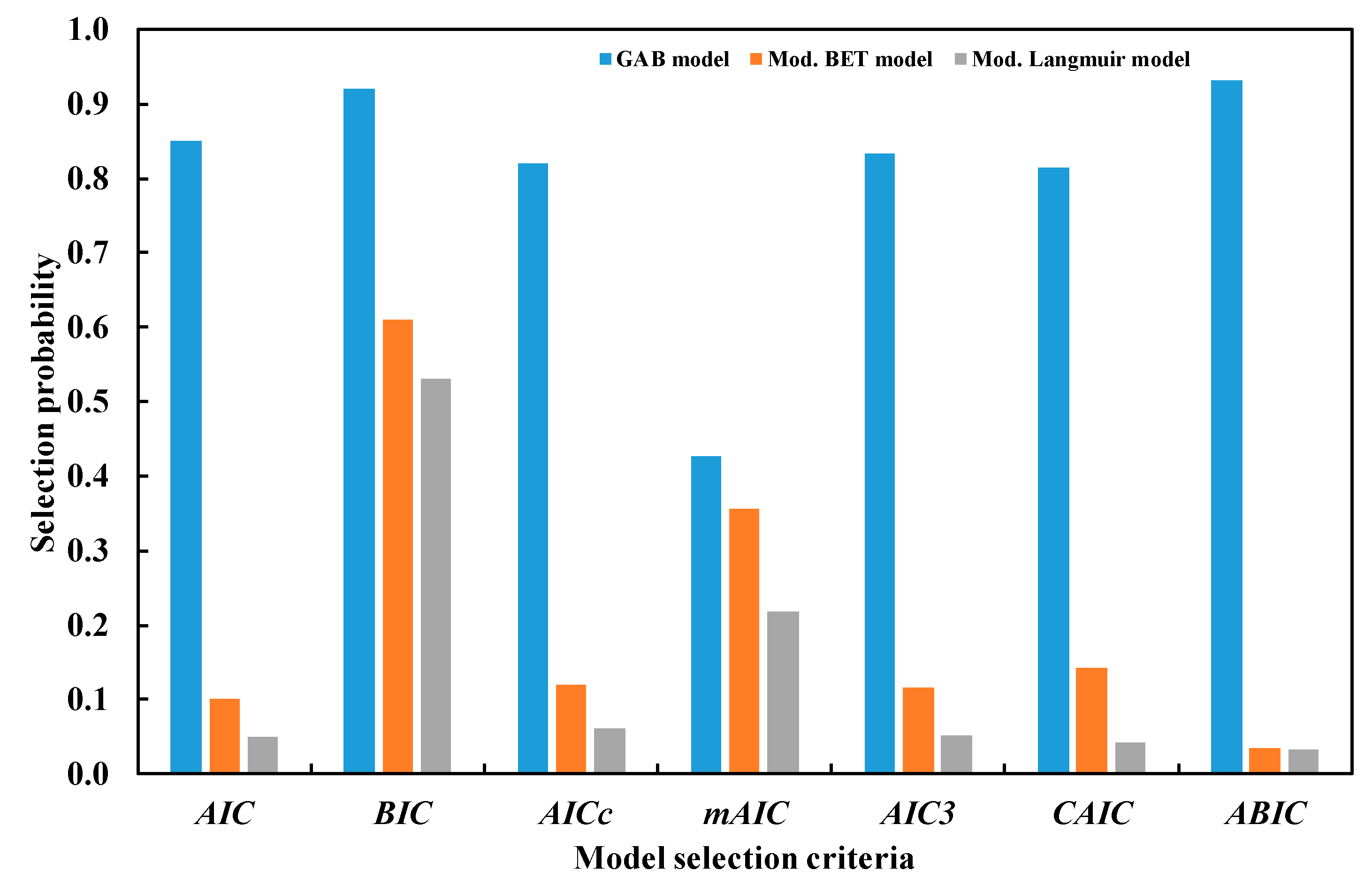
| GAB model | 0.2932 | (0.1720, 0.4280) | −73.10 | −64.66 | −71.34 | −33.10 | −68.10 | −59.66 | −80.30 |
| Mod. BET | 0.8758 | (0.3509, 1.5002) | −33.33 | −28.26 | −32.66 | −21.33 | −30.33 | −25.26 | −37.65 |
| Ng et al. | 1.0613 | (0.6907, 1.4828) | −17.64 | −5.82 | −14.14 | 66.36 | −10.64 | 1.18 | −27.73 |
| D–A | 1.2565 | (0.6192, 2.0008) | −18.89 | −13.82 | −18.22 | −6.89 | −15.89 | −10.82 | −23.21 |
| Sun and Chakraborty | 1.3858 | (0.7615, 2.0736) | −12.97 | −6.22 | −11.83 | 11.03 | −8.97 | −2.22 | −18.73 |
| Mod. Langmuir | 0.7541 | (0.3423, 1.2238) | −31.31 | −19.49 | −27.81 | 52.69 | −24.31 | −12.49 | −41.39 |
| Test | AIC | BIC | AICc | mAIC | AIC3 | CAIC | ABIC |
|---|---|---|---|---|---|---|---|
| Overall | 2.2 × 10⁻¹⁶ | 2.2 × 10⁻¹⁶ | 2.2 × 10⁻¹⁶ | 2.2 × 10⁻¹⁶ | 2.2 × 10⁻¹⁶ | 2.2 × 10⁻¹⁶ | 2.2 × 10⁻¹⁶ |
| GAB vs. Mod. BET | 2.0 × 10⁻¹⁴ | 2.0 × 10⁻¹³ | 2.0 × 10⁻¹⁴ | 2.0 × 10⁻¹² | 2.0 × 10⁻¹⁵ | 2.0 × 10⁻¹⁴ | 2.0 × 10⁻¹⁴ |
| GAB vs. Mod. Langmuir | 2.0 × 10⁻¹⁵ | 2.0 × 10⁻¹⁵ | 2.1 × 10⁻¹⁴ | 2.2 × 10⁻¹⁵ | 2.2 × 10⁻¹⁵ | 2.0 × 10⁻¹⁵ | 2.1 × 10⁻¹⁵ |
| PVDC/water | Mean Error | 95% CI of Error | Tripolis/Water | Mean Error | 95% CI of Error |
|---|---|---|---|---|---|
| Ng et al. | 0.08324 | (0.0486, 0.1210) | Ng et al. | 0.0127 | (0.0043, 0.0247) |
| Yahia et al. | 2.69468 | (1.0143, 4.8338) | Yahia et al. | 0.0903 | (0.0341, 0.1678) |
| Mod. BET | 0.51836 | (0.2596, 0.8222) | BET | 0.2576 | (0.0550, 0.5013) |
| Mahle | 0.92660 | (0.1397, 1.8578) | Mod. BET | 0.1471 | (0.0613, 0.2460) |
| Sun and Chakraborty | 1.12546 | (0.2890, 2.1980) | Do et al. | 0.4532 | (0.0043, 0.0247) |
| Model | Mean Error | AIC | BIC | AICc | mAIC | AIC3 | CAIC | ABIC |
|---|---|---|---|---|---|---|---|---|
| Adsorption of water onto PVDC | ||||||||
| Ng et al. | 0.08324 | −5.50 | 5.96 | −1.77 | 78.50 | 1.50 | 12.96 | −15.93 |
| Yahia et al. | 2.69468 | 31.27 | 44.37 | 36.24 | 143.27 | 39.27 | 52.37 | 19.36 |
| Mod BET | 0.51836 | 4.79 | 9.70 | 5.49 | 16.79 | 7.79 | 12.70 | 0.32 |
| Mahle | 0.92660 | 12.59 | 19.15 | 13.81 | 36.59 | 16.59 | 23.15 | 6.64 |
| Sun and Chakraborty | 1.12546 | 14.54 | 21.09 | 15.75 | 38.54 | 18.54 | 25.09 | 8.58 |
| Adsorption of water onto Tripolis | ||||||||
| Ng et al. | 0.0127 | −34.11 | −22.64 | −30.37 | 49.89 | −27.11 | −15.64 | −44.53 |
| Yahia et al. | 0.0903 | −8.62 | 4.48 | −3.65 | 103.38 | −0.62 | 12.48 | −20.53 |
| BET | 0.2576 | −8.03 | −4.76 | −7.69 | −4.03 | −6.03 | −2.76 | −11.01 |
| Mod BET | 0.1471 | −12.76 | −7.85 | −12.05 | −0.76 | −9.76 | −4.85 | −17.23 |
| IRMOF-74-V-hex/argon | Mean Error | 95% CI of Error | IRMOF-74-V-hex/nitrogen | Mean Error | 95% CI of Error |
|---|---|---|---|---|---|
| Ng et al. | 0.95400 | (0.8126, 0.9967) | Ng et al. | 0.18451 | (0.1124, 0.2435) |
| Mod. BET | 2.71755 | (1.9571, 3.1684) | Mod. BET | 1.19510 | (0.5642, 2.9856) |
| Mahle | 4.24836 | (3.2145, 6.2541) | Mahle | 1.18360 | (0.4265, 3.2113) |
| Mod. Langmuir | 2.68435 | (1.2563, 4.1256) | Mod. Langmuir | 0.53406 | (0.0613, 2.1560) |
| Tόth | 4.34000 | (3.5671, 5.3461) | Tόth | 1.65845 | (0.4125, 2.6571) |
| Model | Mean Error | AIC | BIC | AICc | mAIC | AIC3 | CAIC | ABIC |
|---|---|---|---|---|---|---|---|---|
| Adsorption of argon onto IRMOF-74-A-hex | ||||||||
| Ng et al. | 0.95400 | −48.49 | −37.03 | −44.76 | 35.51 | −41.49 | −30.03 | −58.92 |
| Mod. BET | 2.71755 | −1.01 | 3.90 | −0.31 | 10.99 | 1.99 | 6.90 | −5.48 |
| Mahle | 4.24836 | 24.67 | 31.22 | 25.88 | 48.67 | 28.67 | 35.22 | 18.71 |
| Mod. Langmuir | 2.68435 | 6.34 | 17.80 | 10.07 | 90.34 | 13.34 | 24.80 | −4.09 |
| Tόth | 4.34000 | 25.80 | 32.35 | 27.01 | 49.80 | 29.80 | 36.35 | 19.84 |
| Adsorption of N2 onto IRMOF-74-A-hex | ||||||||
| Ng et al. | 0.18451 | −135.57 | −124.1 | −131.84 | −51.57 | −128.5 | −117.1 | −145.9 |
| Mod. BET | 1.19510 | −44.55 | −39.64 | −43.84 | −32.55 | −41.55 | −36.64 | −49.02 |
| Mahle | 1.18360 | −19.79 | −13.24 | −18.58 | 4.21 | −15.79 | −9.24 | −25.75 |
| Mod. Langmuir | 0.53406 | −79.24 | −67.78 | −75.51 | 4.76 | −72.24 | −60.78 | −89.66 |
| Tόth | 1.65845 | −25.18 | −18.63 | −23.97 | −1.18 | −21.18 | −14.63 | −31.14 |
| Model | Mean Error | CI of HYBRID | AIC | BIC | AICc | mAIC | AIC3 | CAIC | ABIC |
|---|---|---|---|---|---|---|---|---|---|
| D–A | 0.5370 | (0.3538, 0.7506) | −43.21 | −38.46 | −42.46 | −31.21 | −40.21 | −35.46 | −47.83 |
| Mahle | 0.9121 | (0.4822, 1.4353) | −22.14 | −15.81 | −20.85 | 1.86 | −18.14 | −11.81 | −28.30 |
| modified Langmuir | 0.2172 | (0.1225, 0.3370) | −67.79 | −56.71 | −63.79 | 16.21 | −60.79 | −49.71 | −78.58 |
| GAB | 2.6254 | (1.9507, 3.3515) | 13.92 | 18.67 | 14.67 | 25.92 | 16.92 | 21.67 | 9.30 |
| Sun and Chakraborty | 0.1453 | (0.0741, 0.2364) | −88.27 | −81.94 | −86.98 | −64.27 | −84.27 | −77.94 | −94.44 |
| Test | AIC | BIC | AICc | mAIC | AIC3 | CAIC | ABIC |
|---|---|---|---|---|---|---|---|
| Overall | 2.2 × 10⁻¹⁶ | 2.2 × 10⁻¹⁶ | 2.2 × 10⁻¹⁶ | 2.2 × 10⁻¹⁶ | 2.2 × 10⁻¹⁶ | 2.2 × 10⁻¹⁶ | 2.2 × 10⁻¹⁶ |
| Sun and Chakraborty vs. Mod. Langmuir | 2.0 × 10⁻¹⁶ | 2.0 × 10⁻¹⁶ | 2.0 × 10⁻¹⁶ | 2.0 × 10⁻¹⁶ | 2.0 × 10⁻¹⁶ | 2.0 × 10⁻¹⁶ | 2.0 × 10⁻¹⁶ |
| MgO/Methane | Mean Error | 95% CI of Error | Graphite/Methane | Mean Error | 95% CI of Error |
|---|---|---|---|---|---|
| Yahia et al. | 0.1237 | (0.0699,0.1835) | Yahia et al. | 0.562948 | (0.3545,0.7757) |
| Ng et al. | 0.6007 | (0.4107,0.7994) | Ng et al. | 7.848831 | (3.4595,13.359) |
| D–A | 6.6061 | (3.4087,10.022) | D–A | 15.06557 | (9.0459,22.345) |
| Mod. Langmuir | 21.165 | (12.654,30.267) | Mod. Langmuir | 21.242790 | (12.848,30.937) |
| Mahle | 11.430 | (6.3491, 17.249) | Mahle | 12.461560 | (7.7736,17.705) |
| Model | Mean error | AIC | BIC | AICc | mAIC | AIC3 | CAIC | ABIC |
|---|---|---|---|---|---|---|---|---|
| Adsorption of methane onto MgO | ||||||||
| Yahia et al. | 0.1237 | −89.70 | −69.73 | −77.70 | 174.30 | −77.70 | −57.73 | −107.27 |
| Ng et al. | 0.6007 | −26.06 | −4.43 | −11.50 | 285.94 | −13.06 | 8.57 | −45.10 |
| D–A | 6.6061 | 47.45 | 52.44 | 48.13 | 59.45 | 50.45 | 55.44 | 43.05 |
| Mod. Langmuir | 21.1652 | 100.86 | 112.50 | 104.47 | 184.86 | 107.86 | 119.50 | 90.60 |
| Mahle | 11.4302 | 70.83 | 77.48 | 72.00 | 94.83 | 74.83 | 81.48 | 64.97 |
| Adsorption of methane onto graphite | ||||||||
| Yahia et al. | 56.29480 | 159.73 | 181.14 | 169.79 | 423.73 | 171.73 | 193.14 | 143.53 |
| Ng et al. | 784.88310 | 277.66 | 300.86 | 289.80 | 589.66 | 290.66 | 313.86 | 260.12 |
| D–A | 1506.55700 | 286.35 | 291.71 | 286.95 | 298.35 | 289.35 | 294.71 | 282.31 |
| Mod. Langmuir | 2124.27900 | 309.47 | 321.96 | 312.58 | 393.47 | 316.47 | 328.96 | 300.03 |
| Mahle | 1246.15600 | 280.00 | 287.14 | 281.03 | 304.00 | 284.00 | 291.14 | 274.61 |
© 2019 by the authors. Licensee MDPI, Basel, Switzerland. This article is an open access article distributed under the terms and conditions of the Creative Commons Attribution (CC BY) license (http://creativecommons.org/licenses/by/4.0/).
Share and Cite
Rahman, M.M.; Muttakin, M.; Pal, A.; Shafiullah, A.Z.; Saha, B.B. A Statistical Approach to Determine Optimal Models for IUPAC-Classified Adsorption Isotherms. Energies 2019, 12, 4565. https://doi.org/10.3390/en12234565
Rahman MM, Muttakin M, Pal A, Shafiullah AZ, Saha BB. A Statistical Approach to Determine Optimal Models for IUPAC-Classified Adsorption Isotherms. Energies. 2019; 12(23):4565. https://doi.org/10.3390/en12234565
Chicago/Turabian StyleRahman, Md. Matiar, Mahbubul Muttakin, Animesh Pal, Abu Zar Shafiullah, and Bidyut Baran Saha. 2019. "A Statistical Approach to Determine Optimal Models for IUPAC-Classified Adsorption Isotherms" Energies 12, no. 23: 4565. https://doi.org/10.3390/en12234565
APA StyleRahman, M. M., Muttakin, M., Pal, A., Shafiullah, A. Z., & Saha, B. B. (2019). A Statistical Approach to Determine Optimal Models for IUPAC-Classified Adsorption Isotherms. Energies, 12(23), 4565. https://doi.org/10.3390/en12234565