Robust Control Method for DC Microgrids and Energy Routers to Improve Voltage Stability in Energy Internet

Abstract

The energy internet (EI) is a wide area power network that efficiently combines new energy technology and information technology, resulting in bidirectional on-demand power transmission and rational utilization of distributed energy resources (DERs). Since the stability of local network is a prerequisite for the normal operation of the entire EI, the direct current (DC) bus voltage stabilization for each individual DC microgrid (MG) is a core issue. In this paper, the dynamics of the EI system is modeled with a continuous stochastic system, which simultaneously considers related time-varying delays and norm-bounded modeling uncertainty. Meanwhile, the voltage stabilization issue is converted into a robust $H_{\infty }$ control problem solved via a linear matrix inequality approach. To avoid the situation of over-control, constraints are set in controllers. The problem of finding a balance between voltage regulation performance and constraints for the controllers was also extensively investigated. Finally, the efficacy of the proposed methods is evaluated with numerical simulations.

1. Introduction

In the past few decades, the usage of distributed energy resources (DERs) has attracted a significant amount of attention due to their sustainability and environmental friendliness [1,2]. It is notable that the natural characteristics of power generation by DERs, e.g., wind turbine generators (WTs) and photovoltaic panels (PVs), are heavily weather-dependent and over-flexible, which has a significant impact on the accessed conventional power systems [3]. Meanwhile, the convergence of multiple energy resources is the current development trend of future energy systems [4]. For conventional power grids, being able to access renewable energy sources would create challenges in the operation of power grids with conventional power regulation modes, which is why solar power and wind power were previously regarded as ‘waste energy’. To further promote the efficiency of multi-energy conversion and utilization, the architecture of energy internet (EI) is proposed as being the future of the smart grid [5].

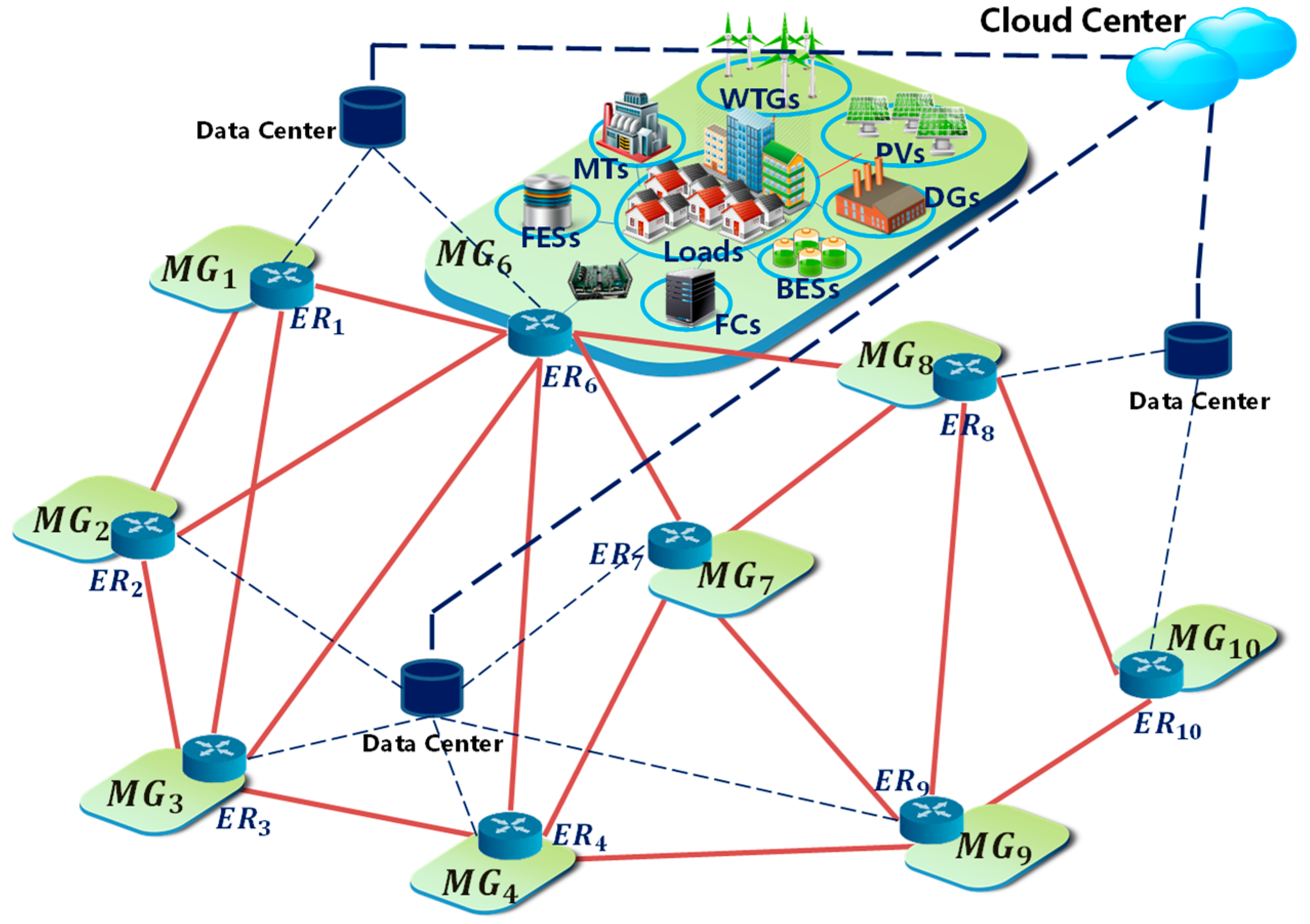
EI is a cyber-physical system inspired by the concept of the Internet, enabling the bidirectional power transmission and on-demand rational energy utilization [6]. Within the scenario of future EI, solar power, wind power and hydro power can be viewed as the main power generation sources, which can be integrated with energy storage devices and various loads. Typically, EI is composed of a utility grid and multiple microgrids (MGs) interconnected via energy routers (ERs). ERs are the core infrastructures of EI systems. The ER, also known as an electric energy router or power router, is a type of electric device that can realize multidirectional power flow and active control of the power flow. In the distribution network, acting as an intelligent interface of distributed power supply, reactive power compensation device, energy storage equipment and load, the ER can flexibly manage the dynamic power in the regional grid network and the whole distribution network on the premise of ensuring power quality. Integration with advanced information technology enables ERs to have communication and intelligent decision-making capabilities. ERs can actively manage the energy flow of the power network according to the operation status of the network and the instructions from the user and control center. The basic function of ER includes plug and play of interfaces, bidirectional transmission; real-time communications and so on. For ERs designed for a backbone network, the main difficulty lies in the technology of high voltage power electronic converters. For small and medium-sized ERs, a high manufacturing cost is the reason why it has not been popularized in the market. The current researches in both academia and industry aim to propose ERs for future energy markets. For a more detailed introduction with respect to ER, readers can consult [6,7,8] and the references therein.

As direct current (DC) MGs not only can improve the power quality and transmission capacity of an EI system but also have superior accesses to DERs, they are more widely used in real projects [9]. Due to the direct influence of power deviation on MG’s DC bus voltage, voltage regulation is usually realized by power control. In an EI scenario, the power balance of the whole system should be achieved by the individual local controllable devices in each MG through prioritizing [10]. However, when faced with extreme conditions, such as a large-scale load power change, MGs tend to be regulated by means of ER operations, which aim to transmit power energy from/to other MGs in order to achieve power supply–demand balance within the whole EI scenario [8,10].

On the other hand, there have been significant achievements in terms of voltage control in related literature, such as [11,12,13,14,15,16]. To illustrate, a local reactive power control scheme that can quickly respond to voltage deviations for preventing communication delay and noise has been previously studied [11]. In [12], the authors proposed voltage control strategies to exploit the cooperation among the agents, such that the power loss minimization objective is achieved. An adaptive control approach for DC MG systems, satisfying both accurate power sharing and voltage regulation, has been previously investigated [13]. Furthermore, a droop-like feedback control method was developed for voltage regulation in [14], enabling the application of theoretical circuits analytical techniques. In [15], with techniques introduced in [17] and the references therein, the problem of voltage regulation is investigated for an islanded MG in EI, which considers system stochasticity and parameter uncertainties.

Naturally, the random change of photovoltaic and wind power as well as the custom of using electricity would stochastically influence PV power output, WT power output and load power, respectively. In [16] and [18], the power of PVs, WTs and loads is modelled using ordinary differential equations (ODEs). As an improvement of ODEs, continuous stochastic differential equations (SDEs) driven by Brownian motions have been applied to model deviations in the power input/output of PVs, WTs and loads in [15,19,20]. In [10] and [21], the Ornstein-Uhlenbeck process was utilized for the power modelling of power fluctuations for PVs and loads.

On the other hand, there are objective measurement errors for any system parameter. When we consider the short-term dynamical properties of the power system, especially for the problem of MG voltage regulation, there is the need for an accurate power dynamical model. Thus, parameter uncertainty must be considered in the dynamical MG model. There exist a variety of approaches to describe parameter uncertainty, such as [22,23]. In this paper, we choose the norm-bounded parameter uncertainty to represent such measurement errors, with the detailed structure introduced in Section 2.

Furthermore, there exists a communication time delay within the information system of EI [6,16]. However, in the aforementioned literature [11,12,13,14,15,16] and the references therein, system stochasticity, parameter uncertainty and communication time delay have not been taken into consideration simultaneously.

In this paper, it is supposed that the considered EI scenario is disconnected with the main power grid and such an EI consists of multiple DC MGs, which are interconnected via ERs. We assume that each MG is composed of PVs, WTs, loads, micro-turbines (MTs), diesel engine generators (DGs), fuel cells (FCs), battery energy storages (BESs) and flywheel energy storages (FESs). The dynamics of the considered system are modelled as continuous differential equations. Due to the randomness of power output of PVs and WTs as well as the stochasticity in the loads, the power deviations of PVs, WTs and loads are modelled as SDEs. We model the dynamics of MTs, DGs, FCs, BESs, FESs and each MG’s DC bus voltage deviations as ODEs. Parameter uncertainties are considered in the system coefficients, which revealed measurement and modelling errors. In addition, the time delay occurring in the communication system is considered in the dynamical equations of the controllable electrical devices. After this, we formulate the voltage control issues in EI as a robust $H_{\infty }$ control problem. The linear matrix inequality (LMI) approach [17] is utilized to solve this problem. Furthermore, the problem of over-control has been concerned and extensively studied. The efficacy of the proposed controller is presented in the numerical simulation.

The main contributions and highlights of this paper are outlined as follows.

(1) The assumption that the EI scenario is functioning without access to main power grid makes the control problem more challenging compared to that with access to the utility grid. Each DC MG is analyzed in detail, with the dynamics of the equipment in MGs (including PVs, WTs, loads, MTs, DGs, FCs, BESs, FESs, ERs) being analyzed. The considered EI dynamical system is complex and authentic, which is reflected in the following three aspects. First, corresponding to the fusion of energy and information in EI, the communication time delay is taken into consideration when formulating the dynamical equations of ERs. Second, when investigating the transient power dynamics in MGs, system modelling errors are accounted. Norm-bounded time-varying parameter uncertainty is used to represent such errors. Third, the stochastic nature of solar power, wind power and loads are fully considered and their power dynamical equations are modelled with SDEs. The voltage regulation issue based on this particular system where communication time delay, system parameter uncertainty and system stochasticity are considered simultaneously has not been considered before within the scope of EI.

(2) We emphasize that our contribution is on modelling and formulating the engineering problem in EI into control issues that we can solve. It is challenging to determine how to transform our considered physical problem in an EI scenario into a control problem itself. The practical voltage regulation problem is converted into a robust $H_{\infty }$ control problem in the time domain. The LMI approach is utilized to solve such a control problem sufficiently in order to achieve both robust stabilization against system internal uncertainty and $H_{\infty }$ performance against external disturbance input.

(3) Based on the sufficient solutions to the robust $H_{\infty }$ voltage regulation issue, an additional constraint regarding the size of controllers was considered, such that the potential over-control for distributed power generators would be effectively avoided. Furthermore, the problem of finding a balance between the voltage regulation performance and the constraints for the controllers has been extensively studied, which has not been considered before. Comparable numerical simulations are performed, demonstrating the effectiveness of the proposed control approach.

The rest of the paper is organized as follows. Section 2 introduces the ER system modelling. Problem formulation and solutions are given in Section 3. In Section 4, numerical examples are illustrated. Section 5 concludes the paper.

2. System Description and Dynamical Modelling

In this section, the system modelling for the considered EI scenario is established.

2.1. EI System Architecture

A typical scenario of the considered EI is given in Figure 1. It is assumed that there are a total of $n$ MGs and $n$ ERs in the considered EI system. The power transmission in the EI system is achieved via the ER network. The structure of the ER network can be described using the terminologies in graph theory. ERs can be seen as the vertices of a graph and the transmission lines between ERs in the ER network can be viewed as the edges in the graph. With the set $V$ defined as $V=\{1,2,\dots ,n\},$ MGs and ERs are numbered as $M{G}_i$ and $E{R}_i$, $i\in V$, respectively.

2.2. System Modelling of Each MG Component

In real-world EI systems, a variety of power generation, energy storage and consumption devices can be installed in MGs. For example, some MGs may have both PVs and WTs installed, while only distributed PVs and MTs are installed for some other MGs. For practical considerations, a certain type of MG system consisting of the most common power devices is considered in this paper. Each MG is supposed to include PVs, WTs, MTs, FCs, DGs, BESs, FESs and loads. In this sense, this type of model could be applicable for various EI scenarios. The power dynamics for these components are introduced below.

2.2.1. Modelling for Power Dynamics of PVs, WTs and Loads

For the $i$th MG, considering the system parameter uncertainty, we use a continuous-time stochastic system to describe the power deviation of PVs, WTs and loads. In this paper, the scalar Wiener processes $w_{PV}^i(t)$, $w_{WT}^i(t)$ and $w_{load}^i(t)$ are utilized to represent the stochasticity in $\Delta P_{PV}^i(t)$, $\Delta P_{WT}^i(t)$ and $\Delta P_{load}^i(t)$, respectively. Based on the models introduced in [15], the power dynamics of $\Delta P_{PV}^i$, $\Delta P_{WT}^i$, $\Delta P_{load}^i$ are expressed as follows:

$$\begin{array}{c}\begin{array}{c}d\Delta P_{\mathcal{M}}^i(t)=\frac{1}{T_{\mathcal{M}}^i}\left[-(1+\Delta a_{\mathcal{M}}^i(t))\Delta P_{\mathcal{M}}^i(t)+v_{\mathcal{M}}^i(t)\right]dt+e_{\mathcal{M}}^i\Delta P_{\mathcal{M}}^i(t)d{w}_{\mathcal{M}}^i(t),\end{array}\end{array}$$

(1)

where $\mathcal{M}\in \{PV,WT,load\}$; $v_{PV}^i(t)$, $v_{WT}^i(t)$ and $v_{load}^i(t)$ are modelled as disturbance inputs with respect to $\Delta P_{PV}^i$,$\Delta P_{WT}^i$ and $\Delta P_{load}^i$. The terms $\Delta a_{PV}^i(t)$, $\Delta a_{WT}^i(t)$ and $\Delta a_{load}^i(t)$ in (1) are bounded time-varying system parameter uncertainties. The time constants $T_{PV}^i$, $T_{WT}^i$, $T_{load}^i$ and system coefficients $e_{PV}^i$, $e_{WT}^i$, $e_{load}^i$ can be obtained with parameter estimation methods.

2.2.2. Power Dynamics of MTs, DGs and FCs

Due to the integration of DERs, which could lead to large power deviation in MG systems, the voltage stability in MGs would become more fragile. In future EI systems, MGs will have a higher penetration rate for renewable energy sources. Thus, it is crucial to ensure the power supply–demand balance in all MG systems. Generally, MTs, DGs and FCs are highly controllable electric devices in common MG systems. By adjusting the output power of these generators, the voltage fluctuations caused by local loads and DERs could be effectively alleviated. Similar to the output power deviation of MTs, FCs and DGs given in [10,15,16], we defined the following equation:

$$\begin{array}{c}\begin{array}{c}d\Delta P_{\mathcal{N}}^i(t)=\frac{1}{T_{\mathcal{N}}^i}\left[-(1+\Delta a_{\mathcal{N}}^i(t))\Delta P_{\mathcal{N}}^i(t)+(1+\Delta b_{\mathcal{N}}^i(t))u_{\mathcal{N}}^i(t)\right]dt,\\ \end{array}\end{array}$$

(2)

where $\mathcal{N}\in \{MT,DG,FC\}$; time constants $T_{MT}^i$, $T_{DG}^i$, $T_{FC}^i$ indicating the response speed of generators could be obtained based on real-world data; terms $\Delta a_{MT}^i(t)$, $\Delta b_{MT}^i(t)$, $\Delta a_{DG}^i(t)$, $\Delta b_{DG}^i(t)$, $\Delta a_{FC}^i(t)$ and $\Delta b_{FC}^i(t)$ are bounded time-varying parameter uncertainties.

2.2.3. Power Dynamics of BESs and FESs

Storage systems are essential pieces of equipment for the normal operation of MG systems. Compared with the controllable power generation devices, such as MTs, DGs and FCs, the energy storage devices have shorter response times [16,20,24]. Thus, BESs and FESs are more widely applied to absorb the power deviation in MG systems.

However, due to the limitations in current energy storage technology, some of the energy storage devices are still relatively expensive [20]. Thus, inappropriate control schemes for BESs and FESs may lead to an increase in the operation costs. For better performance and efficiency, different operation schemes for energy storage systems have been proposed, such as the one proposed in [25]. Most of these works focus on designing control schemes within the energy storage devices themselves, which means that energy storage devices are controlled internally. This is different to the situation in this present paper as no controllers are set in BESs and FESs.

With the similar linearization techniques introduced in [15,18,20], the dynamics of power deviations of BESs and FESs in $M{G}_i$ are given as follows:

$$d\Delta P_{\mathcal{S}}^i(t)=-\frac{1}{T_{\mathcal{S}}^i}\left[(1+\Delta a_{\mathcal{S}}^i(t))\Delta P_{\mathcal{S}}^i(t)+(1+\Delta o_{\mathcal{S}}^i(t))\Delta V^i(t)\right]dt,$$

(3)

where $\mathcal{S}\in \{BES,FES\}$; and $\Delta a_{BES}^i(t)$, $\Delta o_{BES}^i(t)$, $\Delta a_{FES}^i(t)$ and $\Delta o_{FES}^i(t)$ are bounded time-varying parameter uncertainties.

2.2.4. Power Dynamics of ERs

In this paper, ERs are mainly applied for energy exchange among MGs. The functionality of ERs allows the administrator to control the energy flows in the EI system more actively [6,10]. Each MG is assumed to have a connection with an ER, which is interconnected with other ERs. ERs can either function independently or cooperate with other ERs. The energy flow can be transmitted from $M{G}_i$ to $M{G}_j$ via $E{R}_i$ and $E{R}_j$ within the ER network. For any $i<j, i,j=1,2,\dots ,n$, the power transmitted from $E{R}_i$ to $E{R}_j$ at time $t$ is denoted as $P_{ER}^{ij}(t)$. The notation $P_{ER}^{ij}(t)$ with the superscripts satisfying $i\ge j$ will not be used throughout this paper.

The default direction of these power flows could be arbitrarily set and their signs would indicate the actual transmission directions. For example, we are able to set the default power transmission direction between $M{G}_i$ and $M{G}_j$ as from $M{G}_i$ to $M{G}_j$. In this sense, $P_{ER}^{ij}(t)>0$ means that the power is sent from $M{G}_i$ and accepted by $M{G}_j$. Reversely, with $P_{ER}^{ij}(t)<0$, the power flow should start at $M{G}_j$ and end at $M{G}_i$. Based on the default directions, the influences of ERs on the power imbalance in MGs should be calculated accordingly, which would be reflected in (6) and (7).

In the considered EI scenario, the control schemes for ERs and MGs are usually generated by a regional control center in order to achieve better efficiency and flexibility. Delays in transmission lines and communication systems may affect the power flows in the ER network [26,27]. Meanwhile, the power flow in a transmission line might be affected by the engineering environment and ERs at both ends, which is considered as the disturbance for the power dynamics. In this paper, the dynamical power flow $P_{ER}^{ij}(t)$ is approximated as a linear differential equation with control and disturbance inputs, as described in (4). For $i<j,$ $i,j\in V$, we have:

$$\begin{array}{ll}d\Delta P_{ER}^{i,j}(t)& =\frac{1}{T_{ER}^{i,j}}[-(1+\Delta a_{ER}^{i,j}(t))\Delta P_{ER}^{i,j}(t)+v_{ER}^{i,j}(t)\\ & +(a_d{}_{ER}^{i,j}+\Delta a_d{}_{ER}^{i,j}(t))\Delta P_{ER}^{i,j}(t-\tau (t))\\ & +(1+\Delta b_{ER}^{i,j}(t))u_{ER}^{i,j}(t)]dt,\end{array}$$

(4)

where $a_d{}_{ER}^{i,j}$ is a coefficient related to the impacts of the aforementioned delays; and $\Delta a_{ER}^{i,j}(t)$, $\Delta a_d{}_{ER}^{i,j}(t)$ and $\Delta b_{ER}^{i,j}(t)$ are bounded time-varying parameter uncertainties. The notation $u_{ER}^{i,j}(t)$ refers to the controller for the energy transmission between $E{R}_i$ and $E{R}_j$. In (4), the term $\Delta P_{ER}^{i,j}(t-\tau (t))$ reflects the impact of delays in the EI system, where $\tau (t)$ is a time-varying function satisfying $\begin{array}{c}0<\tau (t)\le \mu <\infty ,\end{array}$ and $\dot{\tau (t)}\le h<1.$

2.2.5. Power Dynamics of DC Bus Voltage Deviation

Considering the $i$th MG, we denote the voltage deviation on the power bus of $M{G}_i$ as $\Delta V^i(t)$. According to [28], the voltage on the power bus is influenced by the external power from ERs and the internal power deviation in $M{G}_i$. Thus, the dynamic of $\Delta V^i(t)$ can be formulated as:

$$\begin{array}{c}\begin{array}{c}d\Delta V^i(t)=\frac{1}{T_V^i}\left[(1+\Delta a_V^i(t))(\Delta P_{in}^i(t)-\Delta P_m^i(t))\right]dt,\end{array}\end{array}$$

(5)

where $\Delta a_V^i(t)$ is the bounded time-varying parameter uncertainty; $\Delta P_m^i(t)$ is the power deviation inside $M{G}_i$ defined in (6); and $\Delta P_{in}^i(t)$ is the power input for $M{G}_i$ that comes from $E{R}_i$.

$$\begin{array}{ll}\Delta P_m^i(t)& =\Delta P_l^i(t)-\Delta P_{PV}^i(t)-\Delta P_W^i(t)-\Delta P_{BES}^i(t)\\ & -\Delta P_{DG}^i(t)-\Delta P_{FC}^i(t)-\Delta P_{MT}^i(t)-\Delta P_{FES}^i(t).\end{array}$$

(6)

Based on the adjacency matrix $R$ of the ER network, $\Delta P_{in}^i(t)$ can be expressed as:

$$\begin{array}{c}\Delta P_{in}^i(t)={\displaystyle {\displaystyle \sum }_{j\in V}}{r}_{j,i}{P}_{ER}^{j,i}(t),\end{array}$$

(7)

where $r_{i,j}$ is the element of $R$, indicating the connectivity from $E{R}_i$ to $E{R}_j$.

3. Problem Formulation and Solution

In this section, the voltage regulation problem for the considered EI system is formulated as a robust stochastic control issue. To avoid drastic voltage deviation in MGs, the desired controllers in MTs, DGs, FCs and ERs are sufficiently solved using the robust $H_{\infty }$ control method. Since the obtained sufficient solutions might be too strong, it is possible that the situation of over-control regarding MTs, DGs, FCs and ERs might occur. Thus, some extra constraints for the controllers are proposed in this section in order to successfully avoid the situation of over-control.

3.1. The Mathematical Formulation of EI Dynamical System

Next, the EI system power dynamics is represented with a unified dynamical system, which is introduced as follows. For simplicity, we assume that $w_{PV}^i(t)=w_W^i(t)=w_l^i(t)=w(t), i=1,2,\dots ,n$, which would not lead to significant changes to the considered problem. The similar assumptions are applied in many works, such as [15].

For the $i$th MG, the system state is denoted as the vector $x^i(t)\in {ℝ}^9$, which is defined in (8):

$$\begin{array}{ll}{x}^i(t)\triangleq & [\begin{array}{ccccc}\Delta P_{PV}^i(t)& \Delta P_{WT}^i(t)& \Delta P_{load}^i(t)& \Delta P_{MT}^i(t)& \Delta P_{DG}^i(t)\end{array}\\ & \begin{array}{cccc}\Delta P_{FC}^i(t)& \Delta P_{BES}^i(t)& \Delta P_{FES}^i(t)& \Delta V^i(t)\end{array}]\prime .\end{array}$$

(8)

Similarly, for $M{G}_i$, the disturbance input vector $v^i(t)\in {ℝ}^3$ and control input vector $u^i(t)\in {ℝ}^3$ are denoted as $v^i(t)={\left[\begin{array}{ccc}{v}_{\phi }^i(t)& v_{wind}^i(t)& v_{load}^i(t)\end{array}\right]}^{\prime }\mathrm{and}$ $u^i(t)={\left[\begin{array}{ccc}{u}_{MT}^i(t)& u_{DG}^i(t)& u_{FC}^i(t)\end{array}\right]}^{\prime },$ respectively.

Based on the adjacency matrix $R$, the connections between ERs can be described with two tuples. Suppose that there are a total of $m$ transmission lines in the EI system, we denote the set of the two tuples as $L=\left\{(i,j)\right|i<j, r_{i,j}=1,i,j=1,2,\dots ,n\}.$ We denote the elements in $L$ as $l_1,$ $l_2,$ $\dots ,$ $l_m$, such that the state vector $x^{ER}(t)\in {ℝ}^m$, control input vector $u^{ER}(t)\in {ℝ}^m$ and disturbance input vector $v^{ER}(t)\in {ℝ}^m$ for ERs can be denoted as:

$$\begin{array}{l}{x}^{ER}(t)={\left[\begin{array}{ccccc}\Delta P_{ER}^{l_1}(t)& \cdots & \Delta P_{ER}^{l_i}(t)& \cdots & \Delta P_{ER}^{l_m}(t)\end{array}\right]}^{\prime },\\ u^{ER}(t)={\left[\begin{array}{ccccc}{u}_{ER}^{l_1}(t)& \cdots & u_{ER}^{l_i}(t)& \cdots & u_{ER}^{l_m}(t)\end{array}\right]}^{\prime },\\ v^{ER}(t)={\left[\begin{array}{ccccc}{v}_{ER}^{l_1}(k)& \cdots & v_{ER}^{l_i}(k)& \cdots & v_{ER}^{l_m}(t)\end{array}\right]}^{\prime },\end{array}$$

(9)

respectively. In this sense, we are able to denote the EI system state variable $x(t)\in {ℝ}^{9n+m}$, control input $u(t)\in {ℝ}^{3n+m}$ and disturbance input $v(t)\in {ℝ}^{3n+m}$ of the entire EI system as:

$$\begin{array}{l}x(t)={\left[\begin{array}{cccc}{x}^1{(t)}^{\prime }& \cdots & x^n{(t)}^{\prime }& x^{ER}{(t)}^{\prime }\end{array}\right]}^{\prime },\\ u(t)={\left[\begin{array}{cccc}{u}^1{(t)}^{\prime }& \cdots & u^n{(t)}^{\prime }& u^{ER}{(t)}^{\prime }\end{array}\right]}^{\prime },\\ v(t)={\left[\begin{array}{cccc}{v}^1{(t)}^{\prime }& \cdots & v^n{(t)}^{\prime }& v^{ER}{(t)}^{\prime }\end{array}\right]}^{\prime }.\end{array}$$

(10)

At time $t$, the voltage deviations $z(t)\in {ℝ}^n$ within $n$ MGs in EI are denoted as $z(t)={\left[\begin{array}{ccccc}\Delta V^1(t)& \cdots & \Delta V^i(t)& \cdots & \Delta V^n\end{array}(t)\right]}^{\prime }.$ As the dynamical equations in (1)–(5) are expressed in linear forms, the EI dynamical system can be rewritten into the following explicit form:

$$\{\begin{array}{l}dx(t)=[A(t)x(t)+A_d(t)x(t-\tau (t))+Dv(t)\\ +B(t)u(t)]dt+Ex(t)dw(t),\\ z(t)=Cx(t),\\ x(t)=\varphi (t), -\mu \le t\le 0,\end{array}$$

(11)

where $\varphi (t), -\mu \le t\le 0$ is the initial state. The matrix coefficients in (11) are obtained by:

$$\begin{array}{c}\begin{array}{c}A(t)=A+\Delta A(t),\\ A_d(t)=A_d+\Delta A_d(t),\\ B(t)=B+\Delta B(t),\end{array}\end{array}$$

(12)

with appropriate dimensions. It is assumed that the bounded time-varying uncertainty matrices in (12) satisfies:

$$\begin{array}{c}\begin{array}{c}\left[\begin{array}{ccc}\Delta A(t)& \Delta A_d(t)& \Delta B(t)\end{array}\right]=MF(t)\left[\begin{array}{ccc}{N}_a& N_{ad}& N_b\end{array}\right],\end{array}\end{array}$$

(13)

where $M$, $N_a$, $N_{ad}$ and $N_b$ are real constant matrices while $F(·)$ is an arbitrary time-varying matrix function satisfying:

$$\begin{array}{c}F{(t)}^{\prime }F(t)\le I, t\in {ℝ}^{+}\end{array}$$

(14)

It is notable that the above structure for parameter uncertainties has been used in many works in the field of power systems, such as [15]. Hence, the dynamic system for the considered EI scenario has been explicitly obtained.

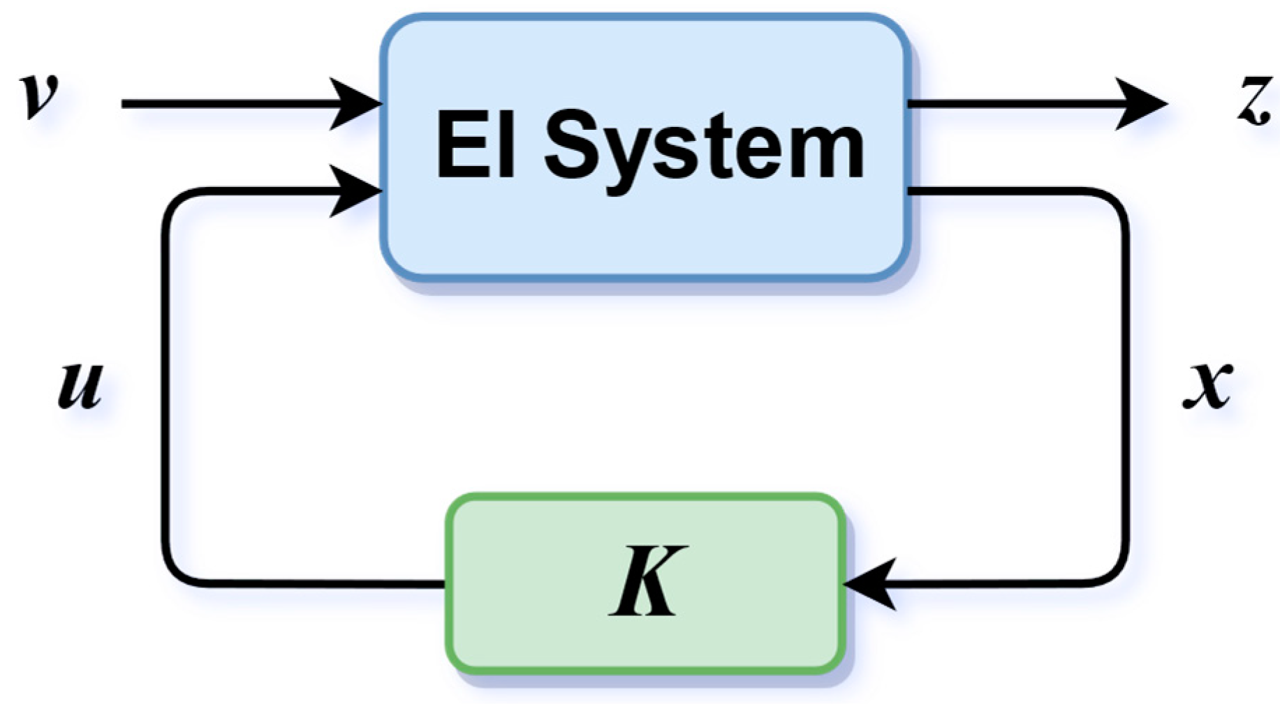
Based on the system modeling given above, a general $H_{\infty }$ control configuration for the voltage regulation problem considered in this paper is shown in Figure 2. The main target of the remainder of this paper is to develop a type of state feedback controller $u=Kx$, such that the controlled output $z$, i.e., the voltage deviations, could be properly restricted in order to remove any influence from the unmodeled disturbance input $v$.

3.2. Robust $H_{\infty }$ Performance

For the considered EI system, the so-called robust $H_{\infty }$ performance particularly refers to the good regulation of the voltage in each MG with respect to two properties: 1) EI system’s internal parameter uncertainty; and 2) external disturbance input from solar irradiation, wind power change, change of electricity usage and disturbing power transmission from other interconnected ERs. Mathematically, we provide a definition of robustly stable (or equivalently, robust stability) for the EI system (11) as follows.

Definition 1:

For dynamical EI system (11), the controlled system with disturbance input$v(t)=0$is said to be robustly stable if for all bounded time-varying parameter uncertainties$\Delta A(t)$,$\Delta A_d(t)$,$\Delta B(t)$in forms of (13),$\underset{t\to \infty }{lim}\mathbb{E}{||x(t)||}_2^2=0$holds. This property is called robust stability. The notation${||\cdot ||}_2$refers to the Euclidean norm.

In addition to the property of robust stability against EI system’s internal parameter uncertainty, the impact of the disturbance input $v(k)$ on voltage deviation should be restricted within certain level, which corresponds to the robust $H_{\infty }$ performance in the control theory. The robust $H_{\infty }$ performance for the investigated EI system is defined in Definition 2.

Definition 2:

For dynamical EI system (11), with a controller$u(x,t)$under a disturbance attenuation level$\gamma >0$, if the controlled EI dynamical system (11) is robustly stable under Definition 1 for all time-varying parameter uncertainties$\Delta A(t)$,$\Delta A_d(t)$,$\Delta B(t)$,$\Delta E(t)$in forms of (11) and if${||z(t)||}_{E_2}\le \gamma {||v(t)||}_{E_2}$holds for all nonzero$v(k)$, where${||z(t)||}_{E_2}={(\mathbb{E}\{{{\displaystyle \int }}_0^{\infty }z{(t)}^{\prime }z(t) dt\})}^{1/2},$the robust$H_{\infty }$performance for the considered EI system is said to be achieved.

The definitions of robust stability and robust $H_{\infty }$ performance introduced above originate from the robust $H_{\infty }$ control theory in the time domain, such as [29]. Following this, the robust $H_{\infty }$ control theory can be applied to obtain the desired controllers. A theorem below is provided to solve our voltage regulation problem.

Theorem 1:

System (11) is robustly stabilized by the linear state-feedback controller$u(x,t)=Y{X}^{-1}x(t)$under the given disturbance attenuation factor$\gamma$if there exist symmetric matrices$X>0$,$S>0$, matrix$Y$and a scalar$\epsilon >0$, such that the LMI in (15) holds:

$$\Gamma <0,$$

(15)

where$\Gamma$is defined in (16),$\mathsf{\Omega }$in$\Gamma$is given in (17).

$$\begin{array}{c}\Gamma \triangleq \left[\begin{array}{c}\begin{array}{cccccc}\mathsf{\Omega }& A_{d}X& D& X{N}_a^{\prime }+Y^{\prime }{N}_b^{\prime }& X{E}^{\prime }& X{C}^{\prime }\\ X{A}_d^{\prime }& -(1-h)S& 0& X{N}_{ad}^{\prime }& 0& 0\\ D^{\prime }& 0& -{\gamma }^{2}I& 0& 0& 0\\ N_{a}X+N_{b}Y& N_{ad}X& 0& -\epsilon I& 0& 0\\ EX& 0& 0& 0& -X& 0\\ CX& 0& 0& 0& 0& -I\end{array}\end{array}\right],\end{array}$$

(16)

$$\mathsf{\Omega }=AX+X{A}^{\prime }+BY+Y^{\prime }{B}^{\prime }+{\epsilon }_{1}M{M}^{\prime }+S.$$

(17)

The EI dynamical system (11) is a special form of the system equation analyzed in [29]. Our obtained theorem can be viewed as a special form of the results in [29]. Thus, the proof is omitted.

The controller obtained from Theorem 1 can be successfully applied to the real-world EI system with guaranteed performance and robustness property. From Definition 2, we can determine that the performance of voltage regulation in the EI system is directly related to the disturbance attenuation level $\gamma$. The controller obtained with a smaller disturbance attenuation level ensures better regulation effect against the disturbances in the EI system.

3.3. Constraints for the Controllers

In [29], it is pointed out that the obtained robust $H_{\infty }$ controllers are sufficient solutions rather than both necessary and sufficient ones, which means that the controller might be excessively strong when a satisfactory robust $H_{\infty }$ performance is achieved. In real engineering practice, voltage stabilization is the main concern in some cases. In order to achieve better power quality, strong controllers are necessary. In some other cases, the magnitudes of the feedback gains should be restricted to avoid the situation of over-control, which might potentially damage the controllable electrical devices.

Thus, in addition to the robust $H_{\infty }$ controllers obtained in Theorem 1, it is necessary to set some constraints in the controllers. Meanwhile, finding a balance between the voltage regulation performance and the constraints for the controllers is still an open problem for the studied system (11), which is investigated below.

Generally, we can manually set the value of disturbance attenuation level $\gamma$ in some applications. The controllers obtained from any feasible solution to (15) can satisfy normal operation requirements in EI systems. However, we would occasionally like to find a controller with the smallest $\gamma$, such that the impacts on DC bus voltages from the disturbance inputs of the EI system can be minimized. This could be achieved by solving the problem in (18):

$$\begin{array}{c}\begin{array}{cc}\min & {\gamma }^2,\\ s.t.& \begin{array}{c}\mathsf{\Gamma }<0\end{array}.\end{array}\end{array}$$

(18)

Supposing the solution to (18) is $X^{(0)},Y^{(0)},S^{(0)},{\epsilon }^{(0)},{\gamma }^{(0)}$, the controller that corresponds to ${\gamma }^{(0)}$ is obtained with $u^{(0)}(x,t)=Y^{(0)}{X}^{(0)}{}^{-1}x(t).$ With $u^{(0)}(x,t)$, the voltage in the EI system (11) should be more stable than that under Theorem 1.

However, a smaller disturbance attenuation level usually suggests larger magnitude of the controller’s feedback gain, which might not be appropriate in real EI scenarios. A feedback controller with large feedback gain might lead to violent adjustments for the distributed generators, which would lead to potential damages. To avoid the situation of over-control, the magnitude of feedback gain needs to be restricted. With Schur complement lemma, it is apparent that:

$$\begin{array}{c}\left[\begin{array}{cc}Q& I\\ I& X\end{array}\right]\ge 0\iff Q-X^{-1}\ge 0,\end{array}$$

(19)

where $Q$ is a symmetric matrix. After this, we have ${||Q||}_p\ge {||X^{-1}||}_p,$ where ${||\cdot ||}_p$ ($1\le p\le \infty$) stands for the $p$-norm. As that the feedback gain $K$ obtained from Theorem 1 satisfies $K=Y{X}^{-1}$, ${||K||}_p^2\le \frac{1}{2}({||X^{-1}||}_p^2+{||Y||}_p^2)$ is established. By minimizing the upper bound for the feedback gain $K$, the intensity of the obtained controller would be consequently restricted, which would reduce the requirement of the proposed controller in practical applications.

Thus, with the idea to minimize $\gamma$ and the LMIs in (15) and (19), we are able to construct a new convex optimization problem as follows:

$$\begin{array}{l}\begin{array}{cc}\min & \eta {\gamma }^2+{||Q||}_p^2+{||Y||}_p^2,\end{array}\\ \mathrm{subject}\mathrm{to}\\ \mathsf{\Gamma }<0,\\ \left[\begin{array}{cc}Q& I\\ I& X\end{array}\right]\ge 0.\end{array}$$

(20)

where $\eta$ is a positive scalar and $p$ is a scalar satisfying $p\ge 1$.

Here, we denote the controller corresponding to the solution to (20) as $u^{(1)}(x,t)$. The solutions to problem (18) and (20) can be obtained with the convex optimization toolbox CVX [30].

4. Numerical Simulation

In this section, the numerical simulations of system (11) is presented to show the efficacy and feasibility of the methods proposed in this paper.

For illustrative purposes, an EI system (without access to utility grid) with four MGs and four ERs is investigated in the following simulation. The considered MGs and ERs are denoted as $M{G}_1$, $M{G}_2$, $M{G}_3$, $M{G}_4$, $E{R}_1$, $E{R}_2$, $E{R}_3$ and $E{R}_4$, respectively.

Let us define the element $\mathcal{A}(i,j)$ of matrix $\mathcal{A}$ as the connectivity between $M{G}_i$ and $M{G}_j$. In this sense, when $M{G}_i$ is connected with $M{G}_j$ via ERs, $\mathcal{A}(i,j)=1$ and $\mathcal{A}(i,j)=0$ otherwise.

The adjacency matrix for the considered EI system is shown as follows:

$$\begin{array}{c}\mathcal{A}=\left[\begin{array}{cccc}0& 1& 1& 1\\ 1& 0& 1& 0\\ 1& 1& 0& 0\\ 1& 0& 0& 1\end{array}\right].\end{array}$$

(21)

Some typical values of time constants and other system parameters in (11) are provided in

Table 1. Typical parameters for devices in energy internet (EI) system.

Parameter	Value	Parameter	Value	Parameter	Value
$T_{PV}$	1.9	$T_W$	1.8	$T_l$	1.6
$e_{PV}$	0.52	$e_W$	0.4	$e_l$	0.6
$T_{MT}$	0.3	$T_{DG}$	0.4	$T_{FC}$	0.5
$T_{BES}$	0.1	$T_{FES}$	0.14	$T_V$	1.2
$T_{ER}$	0.3	$a_{d_{ER}}$	0.05	-	-

. Readers may refer to [15,16,18] for typical MG system parameters. During the simulation, EI system parameters are randomly generated using the product of corresponding parameters in Table 1 and a random variable, which follows the uniform distribution in $\left[0.9,1.1\right]$. To illustrate, the time constants for PVs in these four MGs are 1.9 times the four identically individually distributed random variables within $\left[0.9,1.1\right]$. The time period for simulation is set as $t\in \left[0,10\right]$ (time unit second omitted). The infinity-norm of the parameter uncertainty $\Delta A(t)$, $\Delta A_d(t)$ and $\Delta B(t)$ in system (11) is assumed to be less than 0.05. For the time delay $\tau (t)$ in (11), the constant $h$ is assigned as 0.3. For problem (20), $\eta$ is set to be 10,000. The 2-norm is used to calculate the induced norm for matrices $Q$ and $Y$. In this sense, we have $p=2$.

Based on the dynamical models introduced in Section 2 and the parameters described above, we are able to obtain the parameter matrices in system (11). Both of the solutions to problems (18) and (20) are obtained with the CVX toolbox [29] in MATLAB (R2018b, MathWorks Inc., Natick, MA, USA) environment.

In order to achieve notation simplicity, let us denote the desired controllers solved by problems (18) and (20) as $u^0$ and $u^1$, respectively. When solving problems (18) and (20), the dimensions of the obtained matrices $X$, $Y$ are rather large, which are inconvenient to be explicitly presented in this paper. To show the differences between the solutions to problems (18) and (20), some of the solutions are given in

Table 2. Comparison of solutions for proposed controllers.

Pivotal Parameters	${\mathit{u}}^0$	${\mathit{u}}^1$
$\mathsf{\gamma }$	0.0248	0.133168
$\epsilon$	161.074566	4.940192
${||{YX}^{-1}||}_2$	1743.919809	27.047299

.

In order to show the efficacy of the proposed controllers more intuitively, a detailed analysis is provided as follows.

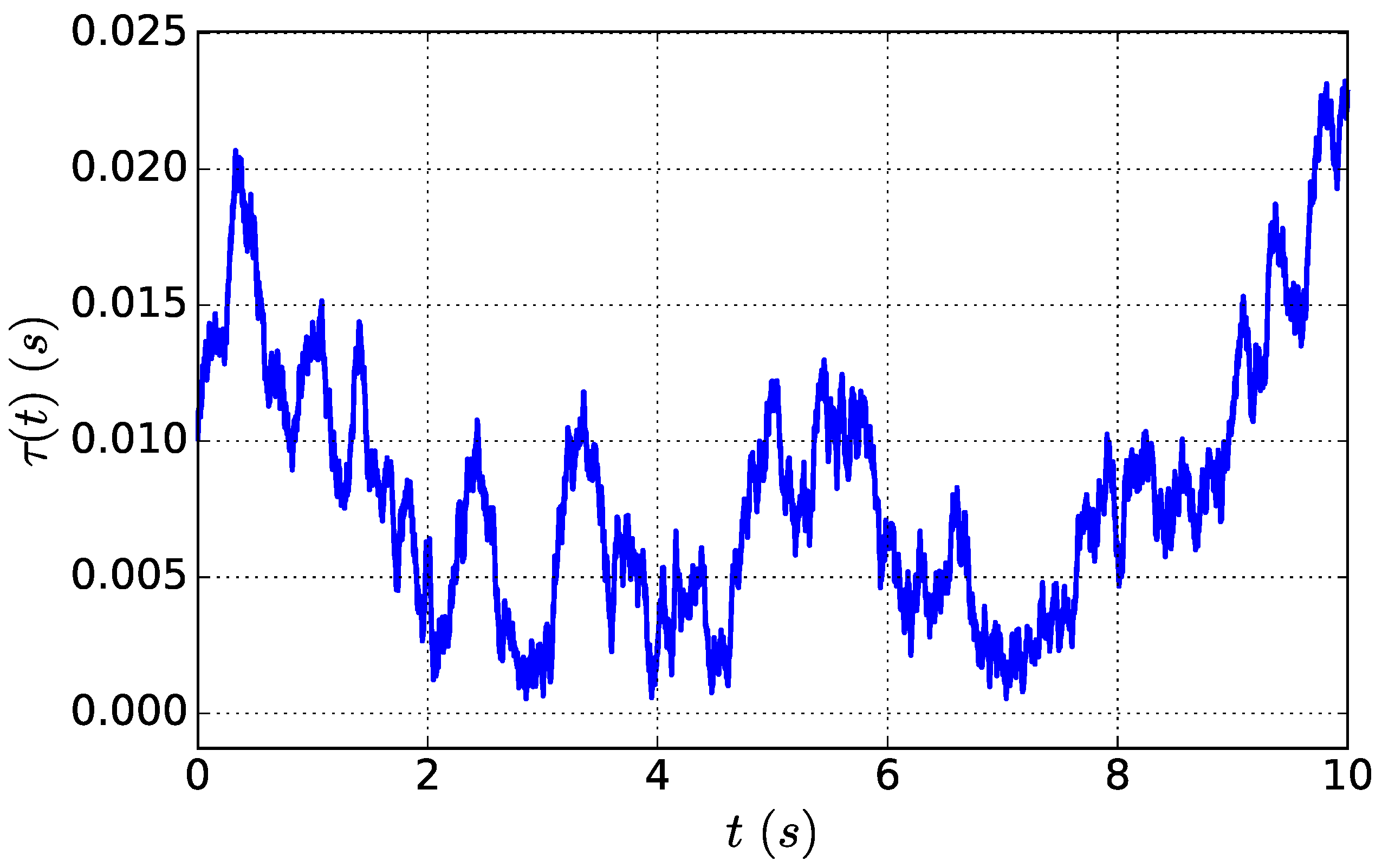
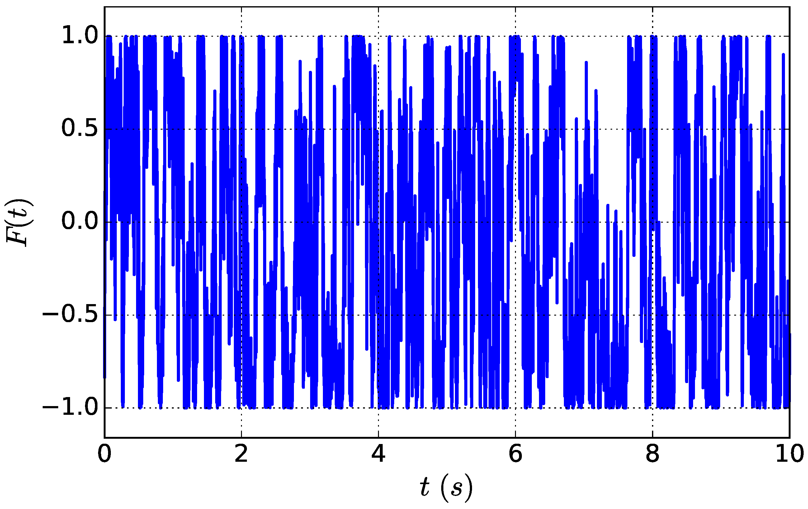
The time delay $\tau (t)$ and the factor $F(t)$ for parameter uncertainties during the simulation period are plotted in Figure 3 and Figure 4, respectively. Basically, the time delay is randomly generated based on the constraints $\begin{array}{c}0<\tau (t)\le \mu <\infty ,\end{array}$ $\dot{\tau (t)}\le h<1.$ For the sake of simplicity, the factor $F(t)$ is generated as a random variable located in $\left[-1,1\right]$.

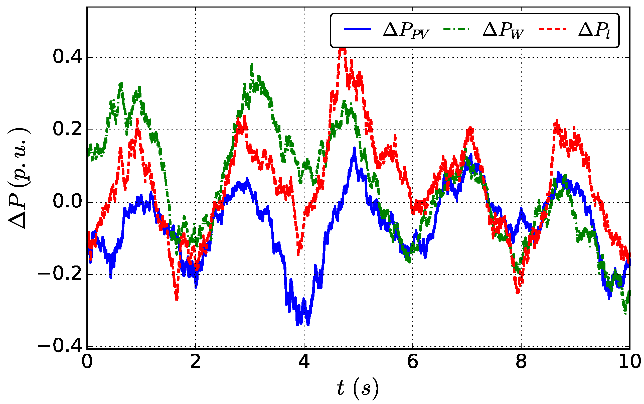
For illustrative purposes, we plot the power deviations of PVs, WTs and loads in $M{G}_1$ in Figure 5. It is clear that the stochastic power characteristics of PVs, WTs and loads are properly approximated.

Based on the curve of time delay $\tau (t)$, factor for parameter uncertainties $F(t)$ and dynamics of PVs, WTs and loads, we are able to evaluate the effectiveness of the controllers obtained from problems (18) and (20) as follows.

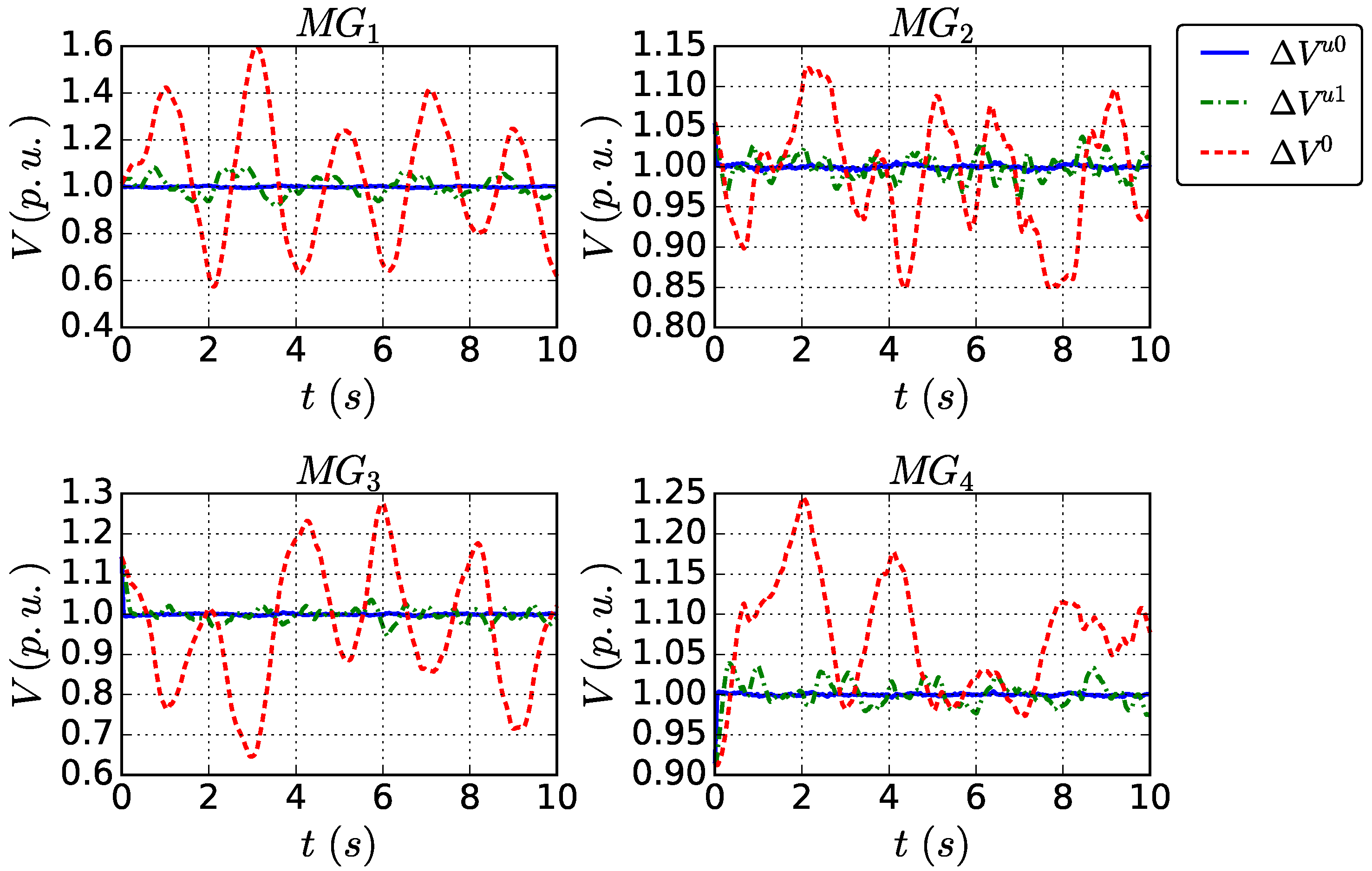
The voltage deviations in four MGs are illustrated in Figure 6. The dashed red curves in Figure 6 refer to the dynamics of voltage deviations when there is no controller applied to the EI system. The dynamics of voltage deviations in the four MGs under $u^0$ and $u^1$ are illustrated with solid blue lines and dashed–dotted green lines, respectively. As stated above, BESs and FESs in MGs are treated as uncontrollable devices. The power deviation in MGs can be absorbed by BESs and FESs. Thus, even if no controller is applied, the voltage deviations in MGs can still be restricted to lie within a relatively small level. However, with the cooperation of generators and ERs, better voltage regulation can be achieved.

In Figure 6, it is obvious that when there is no controller applied, the voltage deviations in MGs are relatively larger. We can also find that both $u^0$ and $u^1$ can effectively achieve the voltage stabilization target. The voltage is further stabilized under $u^0$, which is consistent with the values for disturbance attenuation $\mathsf{\gamma }$ in Table 2. Actually, the disturbance attenuation factor corresponding to $u^0$ is the smallest one that can be achieved with the proposed method. Thus, the stability achieved by $u^0$ is no doubt most excellent.

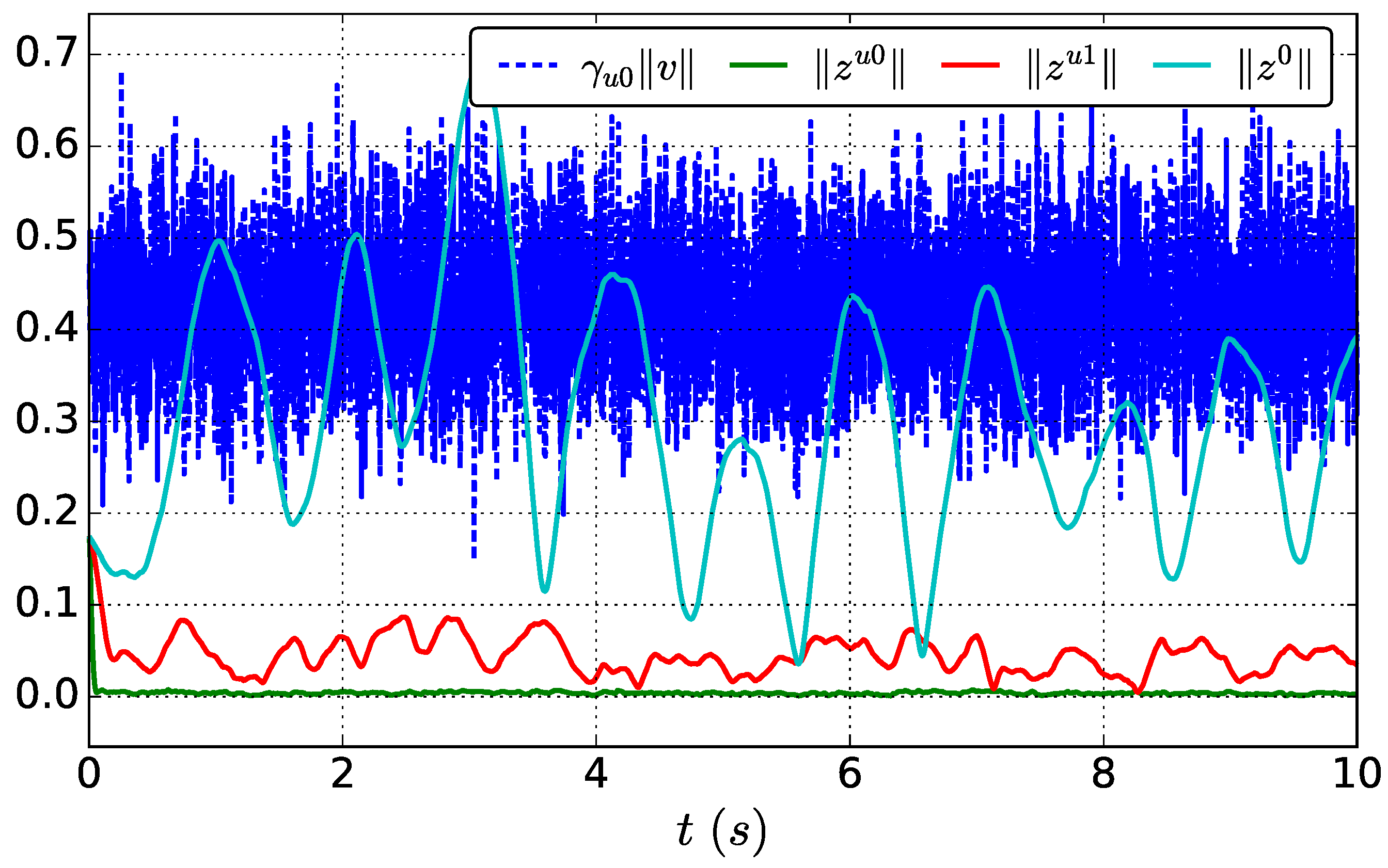
To show the controlled $H_{\infty }$ performance, the quantitative comparison for the norms of $H_{\infty }$ bound ${\gamma }_{u0}||v||$ and observed state $z$ are presented in Figure 7.

In Figure 7, the factor ${\gamma }_{u0}=0.0248$ corresponds to controller $u^0$; $z^0$ is the observation result when there is no control input for system (11); and $z^{u0}$ and $z^{u1}$ refer to the observations of the system (11) when the controllers $u^0$ and $u^1$ are applied, respectively. According to Figure 7, $||z^{u0}||$ and $||z^{u1}||$ are clearly smaller than ${\gamma }_{u0}||v||$, while $||z^0||$ varies in a relative larger range. It is clear that for given disturbance attenuation levels, the studied EI system is robustly stabilized by $u^0$ and $u^1$, respectively. We can find that the deviations of voltage magnitudes exceed the desired upper bound ${\gamma }_{u0}||v||$ at around 3 s. However, the controller $u_1$ with a medium feedback gain effectively maintained the voltage deviations within a small range. Further, the controller $u_0$ with the strongest stabilization ability provides a perfect result as the voltage deviations are nearly zero throughout the simulation period. Based on the results in Figure 7, the controller $u^0$ has much better $H_{\infty }$ performance than $u^1$. However, in order to achieve such excellent $H_{\infty }$ performance against the stochastic disturbances in the considered EI system, the controllable generators, such as MTs and DGs, would be overused, which makes the controller inapplicable in most practical scenarios. Thus, when there is no strict requirement for the voltage stabilization, the controller obtained from problem (15) would provide a satisfactory solution for the EI system management.

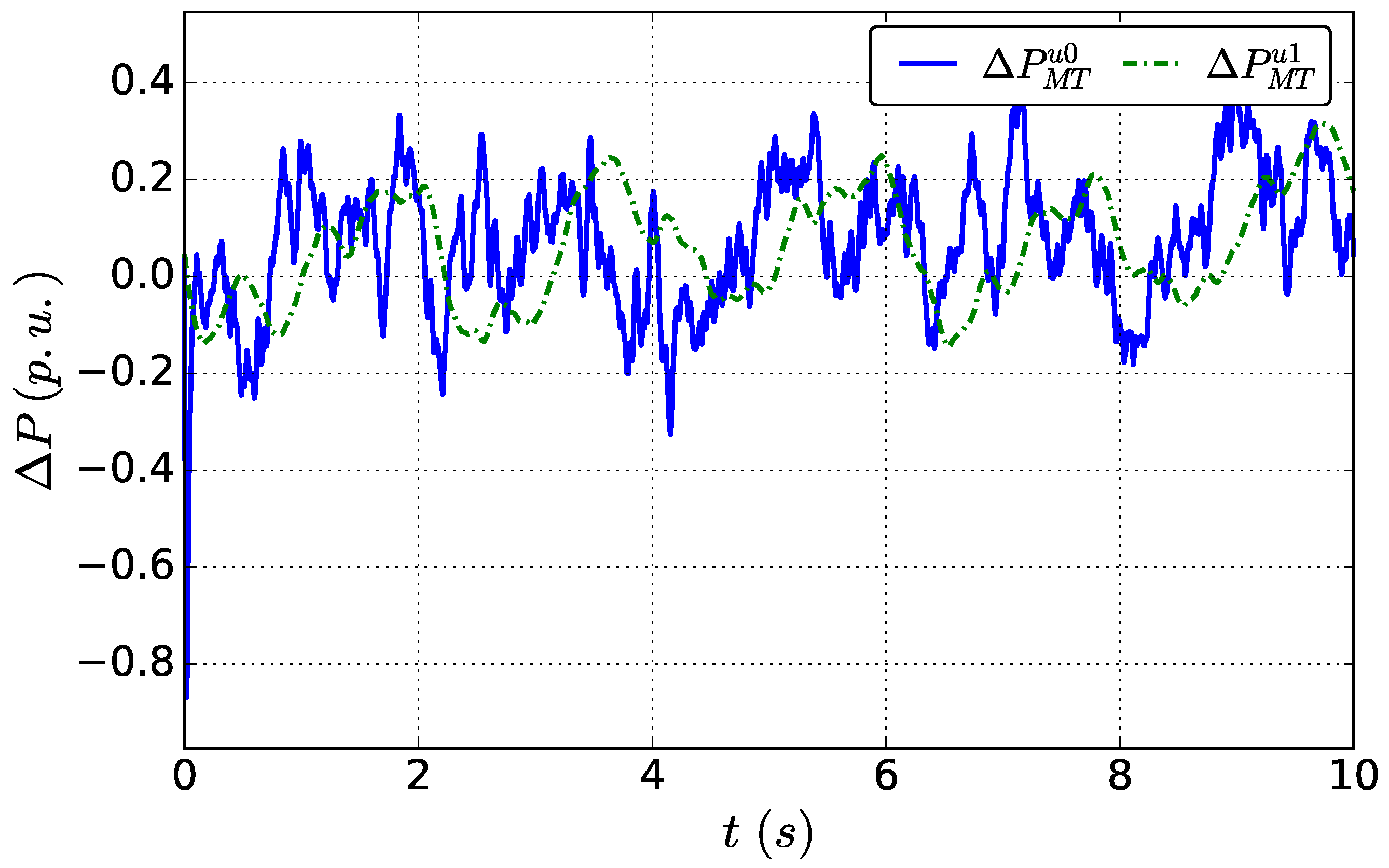
Based on the analysis above, both $u^0$ and $u^1$ have an outstanding effect on the voltage regulation. It is clear that with a smaller disturbance attenuation level $\gamma$, $u^0$ has a better performance. Meanwhile, from Table 2, we found that the feedback gain in $u^0$ is greater. Larger feedback gain usually suggests faster response speed. However, in practical systems, generators, such as MTs, DGs and FCs, sometimes might not be able to accept control signals from $u^0$ as they have large values. In many scenarios, a controller with proper feedback gain would be preferred. To show the differences between the characteristics of the generators under the controllers $u^0$ and $u^1$, the power dynamics of MTs in $M{G}_1$ are given in Figure 8.

From the power dynamic curves in Figure 8, we found that when $u^0$ is applied to the EI system, the generators are able to respond to the voltage deviations faster. Thus, there is vast rapid fluctuations in the curves of MT power output corresponding to $u^0$. On the other hand, when the controller $u^1$ is employed, the output power deviations of generators are more moderate. Thus, we can conclude that controller $u^1$ would be more suitable when the generators are not able to cope with the fast variation of control signals.

In this section, the effectiveness of the proposed control approaches is evaluated with numerical simulations. The performances of the proposed controllers are analyzed. Based on the comparison results, $u^0$ can be utilized in the scenarios with high voltage stability requirements, while it is more suitable to apply $u^1$ in normal EI scenarios.

5. Conclusions

In summary, we transform an industrial EI system into a class of continuous linear SDEs. Both time-varying delays and parameter uncertainties are taken into account. The voltage stabilization issue is formulated as a stochastic robust $H_{\infty }$ control problem and is sufficiently solved. Furthermore, to avoid the potential over-control situations, we conducted an extensive analysis that is focused on designing constraints for the controllers. Simulation results shows the effectiveness of our proposed method.

In this paper, the LMI approach has been adopted to solve a robust $H_{\infty }$ control problem. It appears that the integral quadratic constraint or the Riccati equation based approach could also solve this problem efficiently, such as [31,32]. All these methods would achieve similar stabilization targets. However, due to their different assumptions, the proposed LMI based method would be applicable in some circumstances while the other ones would not and vice versa. Therefore, in practical applications, these methods should be utilized accordingly based on the specific scenarios.

It is important to note that the studied dynamical systems are linear, which is relatively conservative. In fact, all systems in real engineering practice are nonlinear and the technique of linearization itself requires extensive approximations, which creates modelling errors. Furthermore, the centralized state feedback controller requires the access to all system states, which is difficult to achieve in many practical systems. In the future, instead of explicitly establishing dynamical models for the EI system, model-free approaches, such as deep reinforcement learning methods [33], shall be implemented to improve the scalability of conventional centralized control approaches.