Power-mileage-based Algorithm for the Optimization of Distribution Network Structures via Adding Transmission Lines

Abstract

In remote areas, large power stations are often installed to supply local loads due to the difficulties of power transmission. However, with the development of renewable energies and poverty alleviation programs, many renewable energy stations have been installed in such areas. This large amount of surplus and fluctuating energy causes a poor voltage quality, and this problem is difficult to solve with traditional methods. Adding transmission lines can be a feasible solution, but the related research is limited. To provide a guideline for this solution, a network optimization algorithm is proposed in this paper. In the process, a sub-grid that is far from the national grid with an imbalanced power supply and demand is connected to the national grid directly to improve the power quality. First, the linear performance index power mileage is defined to facilitate the calculation and help denote the voltage quality. Then, an iterative algorithm is formed to perform the network optimization and automatically choose the number of clusters. A case study of an actual power grid in Chongqing, China, and an IEEE 123-bus case are used to verify our algorithm. The results show there is a great improvement in the voltage profile.

1. Introduction

Nowadays, power grids face many challenges. New technology enables the grid integration of different renewable energy sources (RESs), which has led to bi-direction power flow and voltage overshoot [1]. The injection of intermittent power into the traditional distribution network has resulted in many problems, and new approaches, including ones that address the allocation strategy, control system, and power grid structure, are needed [2]. Optimization-based power dispatch and battery energy storage systems (BSSs) are frequently used to overcome the poor power quality caused by RESs. However, such approaches may not be efficient in the areas where the output of discrete generators (DGs) cannot be greatly changed and the surplus power generated by the RESs is large. Under such conditions, the optimization of power grid structure can be a promising choice due to its relatively low cost, high flexibility, and efficiency.

Research related to the structure of the power grid can be divided into two types according to the problem being solved. Algorithms for network reconfiguration have been proposed to solve the bi-direction power flow and reduce the power loss in networks [3,4,5,6,7,8,9]. In this approach, a network with loops is designed and switches are used to reconfigure the network so that different radial network is obtained in the running process to re-direct the power flow. The aim of a network reconfiguration is to reduce the total power losses and different optimization algorithms that are applied, including the Particle Swarm Optimization (PSO), Invasive Weeds Optimization (IWO), and Cuckoo Search Algorithm (CSA) [3,4,5]. To address the issue of power losses, the network survivability index was introduced as a measurement of the redundancy, and the Ant Colony Algorithm (ACA) was used to optimize the survivability index and power losses [6]. To achieve a better convergence property, the Big Bang-Big Crunch (BB-BC) [7] algorithm was used, and a mutation step was added to the Big Crunch process. The optimal power losses can be obtained with the modified BB-BC algorithm [8]. In one study [9], a distributed approach was proposed to reconfigure the network based on open shortest path first (OSPF) routing protocol. In that research, the physical architecture was proposed, and the Dijkstra Algorithm was used to obtain the optimal radial configuration.

Algorithms for the network partition were proposed to solve the computational complexity caused by the expansion of the network [10,11,12,13,14,15,16,17]. A large network is partitioned into several clusters in which the supply and demand is balanced, cohesiveness is high, and inter-connection is low so that the control strategy can be applied to each cluster in parallel. Network partitioning requires a distance matrix indicating the dependency of any two nodes. Commonly the differential of the voltage as a function of the power was used as the distance matrix, and the traditional k-means algorithm was applied to achieve the clusters [10]. In one study [11], the usage of the spectral clustering in a power grid was analyzed, and several weight matrixes were proposed and compared. With the normalized Laplacian matrix and its eigenvalues, the first k eigenvectors were chosen to perform the k-means analysis. Similarly, spectral analysis has been applied to address this issue [12], where both the active and reactive matrixes were considered. Instead of using k-means, the Self-Organizing Map (SOM) algorithm was used so that the number of clusters could be learned from the data. A modified community detection algorithm was used to optimize the network partition. An unbiased performance index was proposed with the knowledge of structure and power supply condition in each cluster to determine the quality of the algorithm so that auto-termination of the algorithm was ensured [13]. The sensitivity matrix was used as the distance matrix and different cluster algorithms were compared using four different performance indexes; it was found that intelligence algorithms were superior to classical clustering algorithms [14].

Both the network reconfiguration and network partition help improve the power quality of the modern power grid. However, they need a well predesigned network, which is unrealistic in most rural areas. In underdeveloped areas far from the city center, it is difficult to supply enough energy from the transmission lines, resulting in the exploitation of local resources, such as hydro energy, to compensate for the load demand. However, with the development of renewable energy generators and photovoltaic (PV) poverty alleviation programs, particularly in China, a large number of RESs have been installed in such places, leading to surplus power energy. Such surplus energy is mainly provided by the large hydro station at the end of the grid, which may lead to poor power quality and a voltage overshoot. It is challenging to solve these problems because mainly runoff hydropower stations are installed in such remote areas, and the citizens are not willing to shut down their PVs. To solve the unbalanced power energy at the end of grid, a practical method that has been employed in many places in China is to add transmission lines. By doing so, a power grid is divided into several separated radial grids which are separately connected to a national grid so that the surplus energy can be directly transmitted to the national grid without causing any voltage overshoot. However, research on how to separate a particular network is limited, and the practical operation is based on subjective judgment. Instead of dividing a grid into several inter-connected clusters in the network partition, this problem requires the separation of the unbalanced part of the grid. This paper proposes a power-mileage-based network optimization algorithm to provide a guideline for how to add transmission lines. The main contributions of our work have been illustrated in the following:

(1)

To save the time consumed by calculation, a performance index which denotes voltage profile is deduced and used. It has a linear relationship with the input power condition so that it can be calculated with linear algebra easily.

(2)

A network optimization algorithm is proposed to guide how to divide a power grid and achieve the optimal voltage condition. The algorithms automatically decide the number of clusters and when to stop the iteration.

The rest of the paper is organized as follows. The problem is formulated in Section 2. In Section 3, related concepts, including the power mileage value, are introduced and a simple algorithm to calculate the mileage matrix is also presented. Section 4 elucidates the power-mileage-based algorithm, and two cases are used to illustrate the algorithm’s effectiveness. Section 5 provides another case study, and Section 6 gives our conclusions.

2. Problem Formulation

In rural areas which are far from the city center, there are always some local hydro power stations to provide the local power consumption. However, with the exploitation of RESs and the photovoltaic poverty alleviation program (PPAP), on a large number of windfarms, PVs were installed. Such RESs are often installed locally and the surplus energy provided by the hydro stations could only be transmitted to the national grid, resulting in the voltage overshoot and poor power quality. It is difficult to solve these problems with traditional methods, such as a battery energy storage system (BESS), hydrogen storage system [18] and network reconfiguration, largely because the surplus energy is of the order of 100 MW·h and the structure of the network is already defined. Thus, adding transmission lines can be a promising approach because once an ending large hydro station directly connects to the national grid, the power quality of the grid increases significantly. However, such an intuitive judgment cannot be used as a guideline for real life practice, and a mathematical model is needed to help decide the number of added lines and where to add transmission lines.

Unlike traditional network clustering, which aims to find the best partition of the network with the highest inter-cluster cohesiveness and loosest intra-cluster coupling, network optimization separates the sub-grid, which is far from the national grid and unbalanced in regard to the energy supply and demand. Suppose a grid is divided into $G_1$ and $G_2$, and $G_1$ is the relatively balanced grid originally connected to the national grid. Before the separation, a large amount of power from unbalanced $G_2$ should be transmitted to $G_1$, leading to the voltage overshoot in the ending node of $G_1$. Once an effective separation is made, the power flow through $G_1$ decreases significantly, and a better power quality is achieved. In the meanwhile, the voltage of the first node in $G_2$ will be exactly 1 p.u., instead of the much worse condition before the separation, which also improves the power quality in $G_2$. As a result, an effective separation should offer an improvement of the power quality for all of the sub-grids. The following model of network optimization can be formulated using the above discussion. Suppose that the level of the power quality of a grid $G$ can be quantified with $qua\left(G\right)$, where a smaller value means a better quality, and graph $G$ is separated into $n$ graphs. The following model can be formulated:

$$\begin{gathered} \min f=\max \{qua(G_1),qua(G_2),\cdot \cdot \cdot \cdot \cdot \cdot qua(G_n)\} \\ {G}_1\cup G_2\cup G_3\cup \cdot \cdot \cdot \cdot \cdot \cdot G_n=G \\ \underset{i\ne j}{\forall }{G}_i\cap G_j=\varnothing \end{gathered}$$

(1)

Because only the connected graph without loops is considered, its sub-graph is also a connected graph without loops, which ensures the basic property of a grid. The second and third equations are mutually exclusive and exhaustive of all of the separations; the first equation ensures the power quality of all of the sub-grids to achieve the best conditions. During the flow, a metric power mileage was deduced to quantify the quality of a power grid, and then an algorithm was proposed to perform the separation.

3. Preliminary Work

The graph theory [19] was used to represent a grid. A power grid can be seen as a radial graph where the loads and generators in one position make up the node. The transmission line between two nodes is the branch. The node number is sorted by preorder traversal and the branch order equals the larger one of the two neighboring node numbers. The national grid is node 0 and is not counted. Throughout the whole manuscript, the terms grid, network, and graph have the same meaning and will be used interchangeably.

The definition and calculation of the power mileage are given below.

3.1. Nomenclatures

The terms will be used in the paper will be listed in

Table 1. Nomenclatures of the paper.

Symbol	Explanation
G	it denotes a graph
PMp	active power mileage
PMQ	reactive power mileage
PM	total power mileage
P	power consumption matrix for the whole power grid
M	mileage matrix which denotes structure and the length of lines in a power grid
W	The edge weight matrix of a graph

for a better illustration in the algorithm part.

3.2. Power Mileage

To determine the power quality of a power grid, many different performance indexes have been proposed [20,21,22,23]. In the adding lines problem, we needed a metric to indicate the voltage profile. Because our algorithm will iterate many times, a linear index with input is a reasonable choice. We defined the performance index and power mileage from the voltage drop equation.

The definition of power mileage was deduced from the following:

$$\Delta U_i=\frac{P_i\times R_i+Q_i\times X_i}{U_0}$$

(2)

where $\Delta U_i$ is the voltage drop in a branch, $U_o$ is the normal voltage, $P_i$ and $Q_i$ are the active and reactive power flow through the branch, and $R_i$ and $X_i$ are the resistance and reactance of the line.

For a distribution network in a microgrid, the material and per kilometer’s parameters for the main line typically keep constant due to its relatively small size. To simplify the equation further, the resistance and reactance can be replaced by the resistance and reactance per kilometer (${\rho }_p$ and ${\rho }_Q$) multiplied by the length of a branch ($l_i$) so that the voltage drop between node $n$ and node 0 can be written as

$$\Delta U={\displaystyle \sum _{i=1}^n\Delta U_i}=\frac{{\rho }_p}{U_0}{\displaystyle \sum _{i=1}^n{P}_i\times l_i}+\frac{{\rho }_Q}{U_0}{\displaystyle \sum _{i=1}^n{Q}_i\times l_i}$$

(3)

where branch $i$ is in the path from node 0 to node $n$.

Even if the resistance and reactance per kilometer are not constant in same networks, we can choose one as the base value and then modify the length of other branches to achieve the simplification in Equation (3).

In a particular transmission line, the voltage drop in node $n$ is a linear combination of ${{\displaystyle \sum }}_{i=1}^n{P}_i\cdot l_i$ and ${{\displaystyle \sum }}_{i=1}^n{Q}_i\cdot l_i$ so we called them the active power mileage and reactive power mileage. We calculated the active and reactive power mileage of the whole grid ($P{M}_P$ and $P{M}_Q$) with the method proposed in Section 3.3. Then, the performance index power mileage $PM$ was defined:

$$PM=\tau \times P{M}_P+(1-\tau )\times P{M}_Q$$

(4)

where τ is the weight denotes the relationship between resistance and reactance.

As shown in the formulas, the power mileage has a linear relationship with the power condition so that it can be calculated with matrix. This formula indicates the voltage profile of a power grid and it can be used to optimize.

3.3. Calculation of Power Mileage

We first introduced a mileage matrix ${\left[M\right]}_{n\ast n}$, which describes the structure of the power grid to help the calculation. $n$ is the number of nodes and $M_{ij}$ equals the length of branch $i$ if branch $i$ is part of the path from node 0 to node $j$. Otherwise, $M_{ij}$ is 0.

Column $j$ of ${\left[M\right]}_{n\ast n}$ is the route that arrives at node $j$ from node 0 and the row $i$ of ${\left[M\right]}_{n\ast n}$ means the nodes whose power will transmit through branch $i$. If the power demand of each node is multiplied by the row of the mileage matrix, we can obtain the power mileage in each branch.

Suppose we have an active power condition matrix ${\left[P\right]}_{n\ast t}$, where its element $P_{ij}$ is the power needed in node $i$ at time $j$. As a result, the total active power mileage can be calculated with the following formula (5). In the formula, the row $i$ of ${\left[M\right]}_{n\ast n}$ means the nodes whose power will transmit through branch $i$ (otherwise it will be 0) and the column of ${\left[P\right]}_{n\ast t}$ means the power needed, thus the element $P{M}_{ij}$ of ${\left[PM\right]}_{n\ast n}$ means the active power mileage through branch $i$ at time $\mathrm{j}$.

$$P{M}_P={\displaystyle \sum _{i,j}\left|{[M]}_{n\ast n}\times {\left[P\right]}_{n\ast t}\right|}$$

(5)

The reactive power mileage can be obtained in exactly same way.

3.4. Algorithm to Calculate Mileage Matrix

For the calculation of the mileage matrix ${\left[M\right]}_{n\ast n}$, we needed to decide whether a branch lies in the path between two nodes, which is a time-consuming process. A simple algorithm is discussed here for calculating the mileage matrix from the edge weight matrix of a graph.

Suppose that ${\left[W\right]}_{\left(n+1\right)\ast \left(n+1\right)}$ is the edge weight matrix, and its element $W_{ij}\left(i,j\in \left\{0,1,2\dots n\right\}\right)$ is the length of the branch between node $i$ and node $j$ if it exists. Otherwise, $W_{ij}$ is 0. The pseudocode for algorithm is shown in Algorithm 1.

The effectiveness of this algorithm is briefly explained here. Because this graph is a connected graph without a loop, there exists only one route from node 0 to any node. If $W_{ij}$ is not 0 (line 4), there is a branch $j$ connecting node $i$ and node $j$. The route to node $j$ can be separated into the route to node $i$ plus the branch $j$, and also the route to the node is a column of the mileage matrix, so line 5 and line 6 can be performed to construct a mileage matrix.

Algorithm 1: Calculation of the mileage matrix

Input: edge weight matrix W Output: mileage matrix M n = number of columns in W fori = 1:n  for j = 1:n   $\mathbf{if} W_{ij}!=0$    $M(:,j) = M(:,i)$     $M_{jj}={\mathrm{W}}_{jj}$    endfor  endfor endfor

4. Power-mileage-based Network Optimization

The main task of network optimization is to separate the sub-graph that is far from the national grid and whose power is imbalanced. As we illustrated in Section 2, this means the optimal overall voltage profile, or, minimum power mileage. So, the object of the network optimization algorithms is to find the specific separation of a grid $G$ satisfy:

$$\begin{gathered} \min f=\max \{PM(G_1),PM(G_2),\cdot \cdot \cdot \cdot \cdot \cdot PM(G_n)\} \\ {G}_1\cup G_2\cup G_3\cup \cdot \cdot \cdot \cdot \cdot \cdot G_n=G \\ \underset{i\ne j}{\forall }{G}_i\cap G_j=\varnothing \end{gathered}$$

(6)

where $\mathrm{PM}\left(G_i\right)$ means the total power mileage of $G_i$.

To implement such an idea, an iterative power-mileage-based method is proposed. In each turn, the algorithm only divides the grid into two sub-grids, and thus it works greedily in each turn to find the best separation which satisfies Equation (6) (which is discussed in Section 4.1). In the process of network optimization, there were two issues that needed to be considered: how to choose the best partition and when to stop the iteration. We used an effective indicator in our algorithm, which is explained in Section 4.2.

4.1. Network Optimization Algorithm

The scheme of the algorithm is shown as follows.

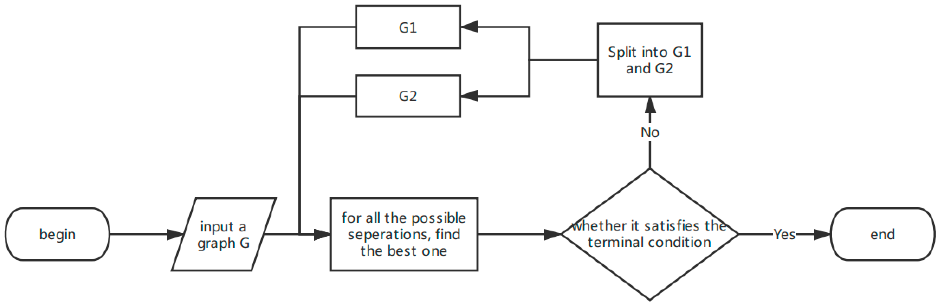
Step 1: For a given graph $G$, each possible candidate for the partition is examined and the best partition is chosen. In this process, $G_1$, $G_2$ and their power mileage $P{M}_1$, $P{M}_2$ are obtained.

Step 2: Check whether the best partition satisfies the terminal condition. If so, graph $G$ is returned. If not, repeat Steps 1 and 2 in graphs $G_1$ and $G_2$ separately.

With the iterative operation and terminal condition, the algorithm can automatically choose the number of clusters and stops when the terminal condition is satisfied. Also, in each iteration, the objective function in Equation (6) is achieved, thus the algorithm greedily finds the optimal separation of the whole grid.

The aim of this algorithm is to separate the sub-graph, which is imbalanced in power and far from the national grid. If the best partition in Step 1 does not satisfy these two purposes, the algorithm should stop. We wanted the power mileage per branch in $G_1$ to be larger than that in $G_2$ so that the imbalance in power is satisfied. We also did not want the voltage profile in the sub-graph to be worse than the original one, so $\max \left\{P{M}_1,P{M}_2\right\}$. should be smaller than $\frac{PM}{2}$. In addition, the number of clusters should not be too large, and the sub-graph should not be too small. In other words, we did not want the algorithm to iterate too many times. As a result, a punishment was added to the second terminal condition. The terminal conditions are not satisfied when both of the following formulas are met.

$$\frac{P{M}_1}{\#(G_1)}<\frac{P{M}_2}{\#(G_2)}$$

(7)

$$\underset{\forall candidates}{\min }\{\max \{P{M}_1,P{M}_2\}<\frac{PM}{2}\times ratio$$

(8)

where $\#\left\{G\right\}$ means the number of nodes in $G$ and $ratio$ means the length of the sub-graph over the length of the original graph.

Equation (7) ensures the imbalance property of the separated graph and Equation (8) ensures the quality of the separation. The existence of $ratio$ punishes the algorithm for splitting the graph too many times. In each iteration, $ratio$ is the length of the graph to be partitioned over the length of the original graph, which is a constant. $ratio$ equals 1 for the first iteration and keeps decreasing in the running process, leading to a heavier punishment.

The flow chart of the algorithm is shown in Figure 1.

4.2. Effectiveness of Terminal Condition

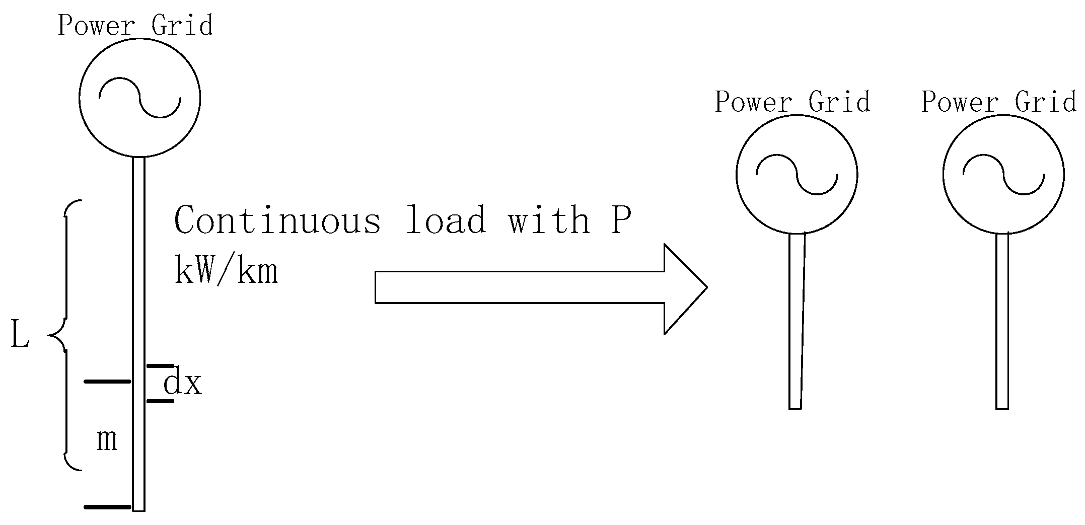
In this part, two cases are used to explain the effectiveness of Equations (7) and (8). For easy calculation, instead of using a discrete load like that found in real life, we used the continuous load, which is distributed evenly in the line. The punishment shown in Equation (6) is not discussed here.

First, a transmission line with evenly distributed loads is discussed (Figure 2). Figure 2 is a model of a traditional distribution network, and it should not be partitioned by our algorithms because the separated grid is exactly the same as the original one. Once a partition is made, the iteration will continue until the end. If we cut the grid at the point that is $m$ km from the end point, the resulting power mileage is calculated as shown in

Table 2. Power mileage for the continuous load case.

	$\mathit{P}\mathit{M}$	$\mathit{P}{\mathit{M}}_1$$\mathbf{or} \mathit{P}{\mathit{M}}_2$	Division
$G_1$	$\frac{P}{2}$	$\frac{P}{2}{(1-m)}^2$	$\frac{m}{1-m}$
$G_2$		$\frac{P}{2}{m}^2$
Sum	$\frac{P}{2}$	$\frac{P}{2}(1-2m(1-m))$

L is set as 1 km. Division is the average power mileage of the second graph over that of the first one. If it is larger than 1, Equation (5) is satisfied.

.

From the power mileage calculation, we can see that when $m=\frac{L}{2}$, the summation of $P{M}_1$ and $P{M}_2$ reaches the minimum and both $P{M}_1$ and $P{M}_2$ equal $\frac{PM}{2}$. As we discussed earlier, the graph should not be separated by our algorithm, so this is the reason why we set the terminal condition as Equation (7). When we cut the graph at $m=\frac{L}{2}$, two parts of the graph are exactly same, so that $G_2$ is not more imbalanced than $G_1$; thus, the division is 1. The above outcome proves the utility of Equation (6).

A network that needs to be partitioned is discussed here. Unlike a pure load system, a large distributed generator (DG) was installed at the end of the grid. The power of the DG was exactly the total load, as shown in Figure 3.

When we cut the line at the same position as the first case, the result in

Table 3. Power mileage for the continuous load case with DG.

	$\mathit{P}\mathit{M}$	$\mathit{P}{\mathit{M}}_1$$\mathbf{or} \mathit{P}{\mathit{M}}_2$	Division
$G_1$	$\frac{P}{2}$	$\frac{P}{2}{(1-m)}^2$	$1+\frac{1}{1-m}$
$G_2$		$Pm(1-\frac{m}{2})$
Sum	$\frac{P}{2}$	$\frac{P}{2}$

L is set as 1 km. Division is the average power mileage of the second graph over that of the first one. If it is larger than 1, Equation (5) is satisfied.

can be achieved.

The summation of $P{M}_1$ and $P{M}_2$ does not change because the absolute value of the power flow through the sub-graph is exactly the same as that of the original one. The only difference is that the flow in the first sub-graph is in the opposite direction compared with that of the original grid. In this graph, our algorithm will cut the line at the point $m=0.293L$ where both $P{M}_1$ and $P{M}_2$ equal $\frac{PM}{2}$. This result is much more reasonable because the power flow through the line in the second sub-graph is much larger, so to reach a better global voltage improvement, the cut point should be closer to the DG. Also, the division is always larger than 1, which means the existence of the DG leads to the imbalance of the second sub-graph.

5. Case Study

To verify the utility of our network optimization algorithm, two case studies were used. The first case study is a 17-node grid in Chongqing, China, and the second one is a classical IEEE case with 123 nodes. The 17-node case was separated using the data for one year and the 123-node case used data at a single time point.

5.1. Study of a real case

A real power grid in Chongqing, China, was used to verify our algorithm. It is a system with 17 nodes and has a total nominal load $1.08 \mathrm{MW}+j0.324 \mathrm{MVar}$. Figure 4 shows the topology of the case with the node number, and

Table 4. Cable parameters.

Type	Length (km)	Resistance (Ω/km)	Inductance (L/km)
Cable 1	1.70	0.435	0.107/314
Cable 2	1.00	0.622	0.113/314
Cable 3	0.05	1.359	0.082/314

shows the information about the cables (cable1 means the cable between two nodes, cable2 means the cable between a node and a transformer and cable3 means the cable between the transformer and the load or generator). To fully consider the change of solar energy and hydro energy in one year, 12 time points were chosen to represent the 12 months of a year.

Two large hydro stations are located in node 11 and node 17, with a total nominal power of $1.2 \mathrm{MW}+j0.59 \mathrm{MVar}$. This is enough power for them to supply all of the load in this area of the country during the high-water season, which is mainly in summer. However, to help the development of this area of the country, PPAP installed 8 PV power stations in the last year, which can generate a total power of $0.502 \mathrm{MW}$. These new installations led to a large amount of surplus energy in the summer. In addition, a large amount of energy is needed in the winter due to the lack of RE and the heavy load. The data over the past year show that the surplus of energy reached nearly $50 \mathrm{MWh}$ in May, with a deficit of $85 \mathrm{MWh}$ in February. Figure 5 shows the power flow through node 0.

To verify the efficient of the power mileage, first the voltage for the ending node (node 17) for 12 months of the real case is calculated by the power mileage and matpower, which uses the Newton-Raphson method. In the deduction of power mileage, approximation is used in the dominator (replace the node voltage with rated voltage), and in the voltage drop equation (use the simplified equation, where only the vertical component is considered). Though in the discussion we illustrate that the influence is small, a test is done on it. The result is shown in Figure 6 and can be seen that two lines are nearly overlapped, which proves the utility of power mileage for its linearity.

We calculated that the total active power mileage $P{M}_p$ is 64845 kW·km and the total reactive power mileage $P{M}_Q$ is 27864 kVar·km. To perform the network optimization algorithm, we chose $\tau$ as 0.8, which denotes the relative magnitude of resistance and reactance. The result of the first iteration is presented in

Table 5. Result of first iteration for the power grid in Chongqing.

Branch		2	3	4	5	6	7	8	9
$PM$	$G_1$	0.3	2.2	2.1	3.0	36.8	36.4	37.4	39.7
	$G_1$	53.6	49.6	45.3	41.2	13.5	12.1	10.2	8.0
Division		10.81	3.05	4.69	4.30	0.67	0.80	0.88	0.94
Maximal		53.6	49.6	45.3	41.2	36.8	36.4	37.4	39.7
Ratio		0.93	0.86	0.79	0.72	0.64	0.63	0.65	0.69
Branch		10	11	12	13	14	15	16	17
$PM$	$G_1$	44.3	42.0	22.1	23.4	23.7	27.0	40.9	46.1
	$G_1$	5.6	2.5	23.5	20.2	16.8	13.5	10.0	5.2
Division		0.95	0.96	1.95	2.07	2.31	2.33	1.83	1.82
Maximal		44.3	42.0	23.5	23.4	23.7	27.0	40.9	46.1
Ratio		0.77	0.73	0.40	0.41	0.41	0.47	0.71	0.80

Division is the average power mileage of the second graph over that of the first one. If it is larger than 1, Equation (5) is satisfied. Ratio is the maximal power mileage value for 2 subgraphs over the original graph’s power mileage. The unit of the power mileage in the table is MW·km or MVar·km.

. In the table, the branch number indicates where the separation is performed. For convenience, we assumed that grid $G_2$ was connected to the national grid from the cutting point.

From the table, we know that cutting the grid at the branch near the smaller hydro station (node 11) is not a good idea because the difference between the supply and demand of power in the sub-graph is not very large, leading to little voltage quality improvement. Only when we cut the grid at branches 12, 13, 14, and 15 could the requirement of Equation (7) be satisfied, and all of them satisfy Equation (6). Separating the grid at branch 13 and adding transmission lines at node 13 were the best choices because we obtained the largest improvement of voltage quality in both sub-graphs. Due to the punishment in Equation (6) and the small scale of the grid, the algorithm stopped at the second iteration, and the final result is shown in Figure 7.

To verify the improvement in the voltage quality, we ran the case study in MATPOWER® for all 12 time points. We chose the two end nodes where the two hydro stations were to show the voltage change after the network optimization. The results are shown in Figure 8.

Figure 8 shows a great improvement in the voltage condition occurs in both node 11 and node 17. In the original power grid, the voltage at node 17 in May transcended the upper limit for the saving operation, which did not occur in the new network. The voltage dip in the winter was greatly alleviated. The large amount of surplus energy made the problem very difficult to solve. Energy at a magnitude of $100 \mathrm{MWh}$ needed to be absorbed, which is a very challenging problem. However, with the help of our network optimization algorithm, the addition of a signal transmission line greatly improved the voltage profile of the grid.

5.2. IEEE 123-bus Case

The classical IEEE 123-bus system was used to verify our algorithm [24,25,26]. We modified the case from a 3-phase unbalanced system to a balanced system and added 6 RESs to the grid [4]. Unlike the case in Chongqing, which had 12 time points that denote 12 months in a year, this case had data only for a single time point. With so many nodes and different lengths of transmission line between each two nodes, this case’ situation is much more complicated. The topology of the case is shown in Figure 9, and the position and the nominal power of the 7 added power stations is shown in

Table 6. Positions and rated power of added generators.

Node	P (kW)	Q (kVar)
32	640	320
38	1610	805
45	1520	760
72	180	0
102	80	0
109	920	560
112	2020	910

.

When $\tau$ equals 0.8464, the network optimization algorithm runs in the 123-bus case. The algorithm also iterates three times, and the power mileage changes from 50.4 to 21.5, where the second value is the maximum power mileage of the sub-graphs and the unit is MW·km or MVar·km. The resulting power grid is shown in Figure 10.

As we assumed, the sub-graphs with large hydro stations were separated from the main grid, and the resulting voltage profile for each node is shown in Figure 11. The voltage quality is much better than the original power grid in every node, and new grids were able to operate in the saving voltage range.

6. Conclusions

In this paper, the problem of adding transmission lines is first discussed. Unlike a well-designed power grid in a big city, power grids in remote areas always include large power stations that supply the demand of local loads. However, with the development of REs and national poverty alleviation programs, these areas usually have a large number of RESs. Without good planning, voltage overshoot and bad voltage quality become the norm. It is difficult to use traditional methods to overcome such problems due to the large amount of energy being managed. However, adding transmission lines is a promising method. In our study, a network optimization algorithm is proposed to present a guideline for adding transmission lines. In this process, the sub-graph that is far from the national grid and imbalanced between the power supply and demand is separated and connected to the national grid directly. To measure the quality of a network partition and facilitate the calculation, the power mileage value is deduced from the voltage drop equation. It has a linear relationship with the power flow and can indicate the voltage quality of a power grid. Then, an iterative algorithm is proposed to perform the network optimization. The algorithm can automatically choose the number of sub-graphs, and the effectiveness of the terminal conditions were verified by several case studies. We evaluated the algorithm using a real grid with 17 nodes and the IEEE 123-bus grid. Our results show a great improvement in the voltage profile for both cases and proves the utility of the power mileage value.