Decentralized Optimal Control of a Microgrid with Solar PV, BESS and Thermostatically Controlled Loads

Abstract

Constructing microgrids with renewable energy systems could be one feasible solution to increase the penetration of renewable energy. With proper control of the battery energy storage system (BESS) and thermostatically controlled loads (TCLs) in such microgrids, the variable and intermittent energy can be smoothed and utilized without the interference of the main power grid. In this paper, a decentralized control strategy for a microgrid consisting of a distributed generator (DG), a battery energy storage system, a solar photovoltaic (PV) system and thermostatically controlled loads is proposed. The control objective is to maintain the desired temperature in local buildings at a minimum cost. Decentralized control algorithm involving variable structure controller and dynamic programming is used to determine suitable control inputs of the distributed generator and the battery energy storage system. The model predictive control approach is utilized for long-term operation with predicted data on solar power and outdoor temperature updated at each control step.

1. Introduction

The inherent variability and intermittency of renewable power could be the major issue to hinder its penetration. One feasible solution is to construct more microgrids integrated with battery energy storage systems (BESSs) and renewable energy systems (RESs), which allows the renewable energy to be smoothed and used locally without interfering with the utility power grid [1]. With the help of predicted renewable energy, electricity price, and load demand, proper control of BESS at different time intervals could minimize the overall energy cost. There has been some research taken under this scheme. The paper [1] proposed an energy trading strategy for a microgrid. They considered different electricity prices from six RESs at different dispatching intervals to determine the actions of a BESS to meet the power demand at a minimum cost. An energy management strategy for a microgrid community is introduced in [2], which consists of multiple microgrids integrated and regulated with a community energy management system. The authors utilize day-ahead forecasting data to plan the desired controls for all units in those microgrids, including output power of distributed generators, charging/discharging power of BESSs and power exchanged between them. An energy scheduling model of microgrids with renewable generations and BESSs is proposed in [3], in which the storage system is considered as the spinning reserve to smooth the power fluctuations due to the intermittent renewable generators, and the authors utilized chance-constrained programming to solve the stochastic optimization problem efficiently. A bi-level energy scheduling strategy for microgrids with battery swapping stations of electric vehicles is introduced in [4], in which the net costs of the microgrid is minimized in the upper-level, and the profits of the battery swapping stations are maximized based on real-time pricing.

Thermostatically controlled loads (TCLs), such as air conditioners, heaters, and ventilation systems, are some of the most widely used electrical appliances [5]. In microgrids with intermittent energy, they could provide the required ancillary services for renewable generation balancing, which could be more flexible than conventional generators that are often constrained by their capabilities [6]. Furthermore, in energy markets with demand response programs, due to the inherent flexibility of TCLs, they are well-suited for consumers to adjust energy usage in response to electricity prices or incentive payments [7].

In this paper, we focus on the control of TCLs in the microgrid environment. The primary objective is to maintain the desired temperature at residential buildings in a cost-effective manner. These TCLs are powered by a distributed generator (DG) and a solar power system, and a BESS is used to regulate the actual power dispatched to them. We consider an islanded microgrid environment, and there will be no power exchanged from the microgrid to the unity grid. As a result, over periods without solar energy, the TCL units will be supplied only by the generator and the BESS, so there will be a non-zero minimum output requirement for the generator to avoid start-up or shut-down cost. In addition, as the residential TCLs are generally constructed in a large quantity with relatively small capacity in practice, it can be complicated and inefficient for the microgrid operator to control each TCL directly. Therefore, the aggregation model of distributed TCLs is used in many studies [8,9,10].

Authors of [8] propose a two-stage optimization model for a group of TCLs to smooth the power fluctuation resulting from PV systems in distribution networks. In the first stage, the regulation capability of TCL groups is determined from the aggregation of user inputs including the change in the temperature set points and maximum allowed temperature, which is then used to calculate the required regulation power to smooth the net exchange power fluctuation at a minimum cost. In the second stage, the regulation task is decomposed to each TCL group. A short-term operation model of the microgrid with high penetration of solar power and TCLs is introduced in [9], which schedules the distributed generator, BESS and TCLs in the microgrid based on solar power forecasting. The receding horizon optimization technique is utilized to alleviate the effects of forecasting errors. The use of aggregated TCLs in the wholesale electricity market is discussed in [10], and an aggregator determines the volume of electricity exchanged with the market in the next day based on renewable generation and load forecast. The objective is to maintain the suitable water temperature for prosumers at a minimum energy cost, and a model predicted control optimization is applied intraday to minimize the imbalance between the forecast data and the actual measurements.

Most of these studies can be perceived as the multi-objective control problem, with temperature control from TCLs being one primary target. Others can be the overall optimization in different environments such as microgrid and deregulated energy market. Since predicted data on renewable power, electricity price and load demand are used in their algorithms, one of the main challenges in these studies can be the errors in forecasting. To address this, the receding horizon approach is utilized in most studies [8,9,10,11,12,13,14,15], as uncertainties can be reduced to a relatively low level with constantly updated forecasting data. Nevertheless, this approach has a strict requirement for the computation time as the set of results over a forecasting horizon should be solved before the first control step over the horizon expires. In practice, delays due to forecasting techniques, data communications, and response time in power electronics can further degrade the performance of the algorithm.

In this paper, we propose a novel decentralized algorithm for optimal control of microgrids with high solar power penetrations and TCLs. We aim to solve our problem in one stage optimization. With the aggregation of TCLs, only the outdoor temperature is required to calculate the power demand, which reduces the computation time spent on the TCL model. As other units in the microgrid, such as renewable energy system, BESS, and distributed load, have cost models related to their control signals and states, the objective function of the optimization problem can be an additive cost over the forecasting horizon. Therefore, we formulate the problem in a cost-to-go equation, or the dynamic programming type equation to solve the sets of controls for both BESS and DG based on forecasting data over each horizon. As the model predictive control approach is applied, only the first component of both sets will be used as the actual inputs to the system in the current stage, and the algorithm will repeat in the next step with updated system states and predicted data. A critical feature of our approach is that TLCs are controlled in a totally decentralized fashion and only the indoor temperature in the corresponding area is needed to control each TCL. Moreover, control of the distributed generation unit and charge/discharge of the BESS does not require any information on the current indoor temperatures.

The remainder of the paper is structured as follows. Section 2 introduces the overall optimization problem. The control system and the cost model of each unit in the microgrid are described in Section 3. The proposed decentralized variable structure/dynamic programming control algorithm and the simulation results are introduced in Section 4 and Section 5, respectively. The last section concludes the paper.

2. Problem Statement

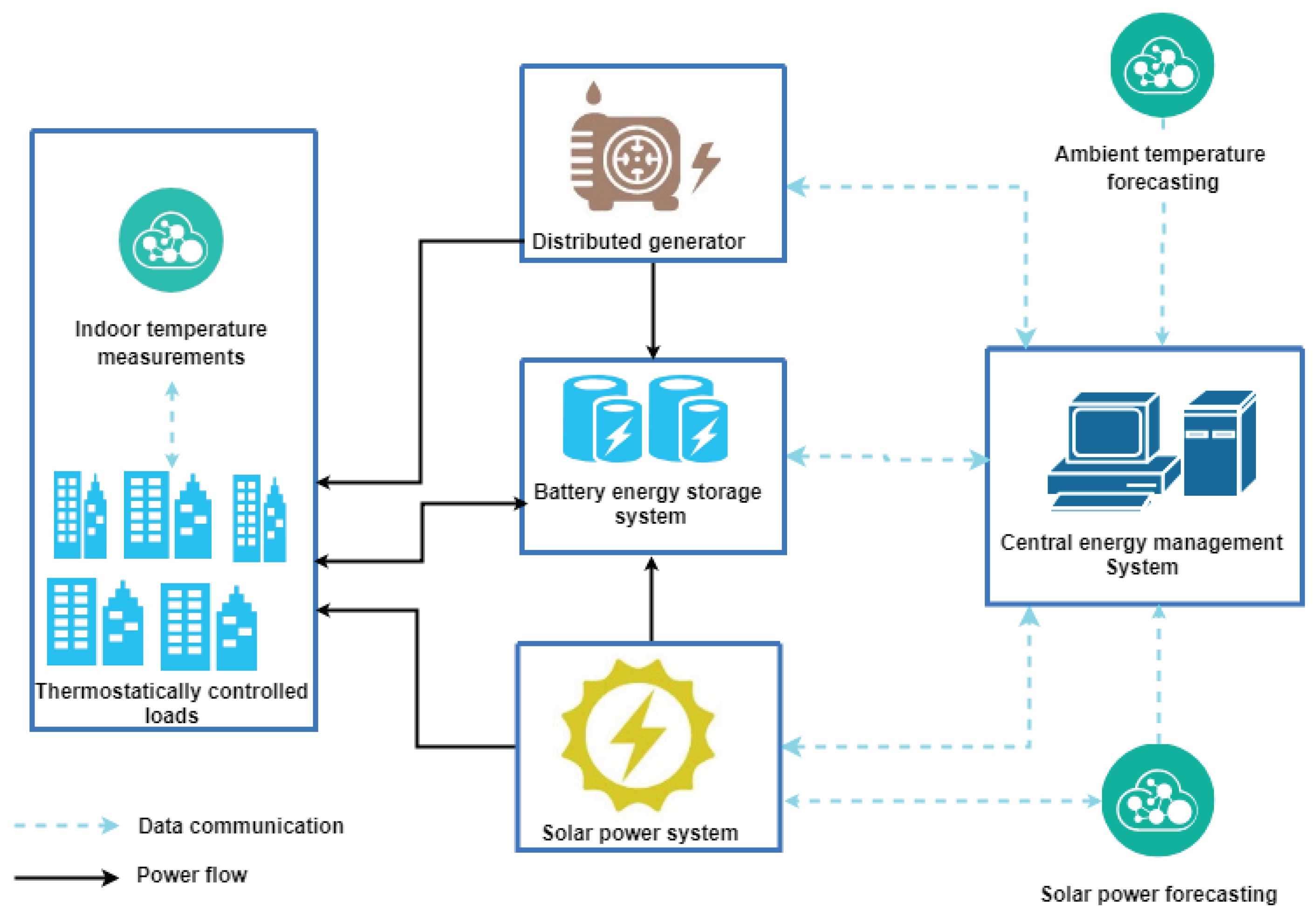
We consider a microgrid consists of a distributed generator (DG), a battery energy storage system (BESS), a solar power generation unit, and a group of thermostatically controlled loads (TCLs). An islanded microgrid environment is considered, and the TCLs are supplied by the solar power system, DG and BESS without power exchanged from the microgrid to the unity grid. The main objective is to minimize the overall cost required to keep the desired building temperature. The configuration of the microgrid is presented in Figure 1.

A decentralized control scheme is used, in which the central energy management system would receive predicted data on solar power and outdoor temperature over a forecasting horizon, and the control inputs for the DG, BESS, and TCLs over the period are then solved based on the predicted data. The DG and the BESS have cost models related to their output power and charging/discharging power, which are controlled following the predicted solar power to meet the power demand from TCLs. In the corresponding areas of TCLs, the indoor temperature is controlled to slide along the setpoint. In addition, the receding horizon approach is utilized for long-term operation, with predicted data updated at each control step.

Since the objective is to minimize the overall energy cost, the additive costs from both DG and BESS over each forecasting horizon is used as the objective function. Based on predicted solar power and outdoor temperature, a dynamic programming (DP) algorithm is used to solve two sets of optimal controls for both DG and BESS, which are the output power of DG and the charging/discharging power of BESS respectively. As the receding horizon approach is used, only the first component of both sets will be used as actual inputs to the system at the current stage, and the algorithm will repeat in the next control step with updated system states and predicted data.

3. System Model

The control system model of the microgrid is introduced in this section.

3.1. Distributed Generator

The cost of the generator used in the microgrid is described by the following function:

$$C_G\left(P_G\left(t\right)\right)=a{P}_G{\left(t\right)}^2+b{P}_G\left(t\right)+c$$

(1)

where $P_G\left(t\right)$ is the power output of DG at time $t;a,b,$ and c are generation cost coefficients of DG. We consider our system as a discrete-time system with the sampling rate $\delta >0$, So the function $P_G\left(t\right)$ is supposed to be piecewise constant with constant values over periods $[k\delta ,(k+1\left)\delta \right)$. Hence, the cost of generation over time interval $[k\delta ,(k+1\left)\delta \right)$ is

$$\sum _{k=k_0}^{N-1}a{P}_G{\left(k\delta \right)}^2+b{P}_G\left(k\delta \right)+c$$

(2)

In addition, the power output of DG should always satisfy the constraints:

$$P_G^{min}\le P_G\left(t\right)\le P_G^{max}$$

(3)

with some given constants $0<P_G^{min}\le P_G^{max}$.

3.2. Battery Energy Storage System

We refer to the battery model introduced in [9], and the dynamics of BESS used in this study is described by the following equation:

$$x\left((k+1)\delta \right)=x\left(k\delta \right)-P_B\left(k\delta \right)\Delta t+d|P_B\left(k\delta \right)\Delta t|,$$

(4)

where $x(·)$ represents the available energy stored in BESS, $\Delta t$ is the factor used to convert power to energy based on the actual time of each control step, $P_B(·)$ is the charging/discharging power of the BESS, $d>0$ is the charging/discharging loss factors of the BESS. Based on the model, $P_B(·)>0$ indicates the discharging action and $P_B(·)<0$ indicates the charging action of BESS.

Based on the cost model introduced in [16], the operational cost of BESS over the time interval $[k\delta ,(k+1\left)\delta \right)$ is modelled as:

$$\sum _{k=k_0}^{N-1}{\gamma }_1|P_B\left(k\delta \right)\Delta t|+{\gamma }_{2}x\left(k\delta \right),$$

(5)

where ${\gamma }_1>0$ and ${\gamma }_2>0$ are some given constants calculated based on the battery life degradation [16]. In addition, the following constraints should be satisfied:

$$P_B^{min}\le P_B\left(t\right)\le P_B^{max}$$

(6)

$$x^{min}\le x\left(t\right)\le x^{max},$$

(7)

where $0<x^{min}<x^{max}$ are the upper and lower limits of the BESS energy state.

3.3. Solar Power Generation Unit

As the receding horizon approach is applied, it is assumed that prior to every control horizon, a predictive estimate $P_s\left(t\right)$ of the power output from the PV system can be made over periods $[k\delta ,(k+1\left)\delta \right)$, which is supposed to be piecewise constant with constant values. In addition, the maximum power that can be supplied from the solar power system is $P_s^{max}$. Since the receding horizon approach is used, some fast forecasting methods would be required to produce accurate results over a relatively short period, such as the techniques introduced in [17,18,19].

3.4. Thermostatically Controlled Loads

The microgrid also contains n thermostatically controlled loads, labelled by $i=1,2,\dots ,n$. Based on previous research [6,8,9], we use the following continuous time equation to describe their dynamics:

$$\dot{T_i^{in}}\left(t\right)={\alpha }_i(T^{out}\left(t\right)-T_i^{in}\left(t\right)-{\beta }_i{s}_i\left(t\right)P_i)$$

(8)

where $T^{out}\left(t\right)$ is the outside temperature at time t, $T_i^{in}\left(t\right)$ is the indoor temperature of the TCL i at time t. $P_i$ is the rated power of the TCL i, $s_i\left(t\right)$ is the ON/OFF state of the TCL i at time t (0-OFF, 1-ON), ${\alpha }_i>0$, ${\beta }_i>0$ are given constants based on Equation (8) in [9]. One of the control goals is to keep the indoor temperature in a comfortable range:

$$D_1\le T_i^{in}\left(t\right)\le D_2,\forall t,i,$$

(9)

where $D_1<D_2$ are given constants. Moreover, we assume that

$$T^{out}\left(t\right)\ge D_2,\forall t,$$

(10)

Furthermore, all initial indoor temperatures satisfy

$$T_i^{in}\left(0\right)\ge D_2,\forall t,$$

(11)

It is also assumed that we have a predictive estimate ${\widehat{T}}^{out}\left(t\right)$ of the outside temperature $T^{out}\left(t\right)$, the function ${\widehat{T}}^{out}\left(t\right)$ is piecewise constant with constant values over periods $[k\delta ,(k+1\left)\delta \right)$. Therefore, the total TCL unit power consumption over the time interval $[k_0\delta ,(N-1)\delta )$ is defined as:

$$\sum _{i=1}^n(P_i{\int }_{k_0\delta }^{(N-1)\delta }{s}_i\left(t\right)dt)$$

(12)

4. Optimization Problem

The system control inputs include the DG power output $P_G\left(k\delta \right)$, the charging/discharging power of the BESS $P_B\left(k\delta \right)$, and the switching functions $s_i\left(t\right)$ of the TCLs. In addition, the additive costs from both DG and BESS can be considered as the output of the system.

Among these inputs, the switching function $s_i\left(t\right)$ varies based on the measurement of the indoor temperature $T_i^{in}\left(t\right)$ only. The control variable $P_G\left(k\delta \right)$ and $P_B\left(k\delta \right)$ are selected based on measurements of $x\left(k\delta \right)$, predictive estimates ${\widehat{T}}^{out}\left(t\right)$ and $P_s\left(k\delta \right)$ of the outside temperature and the power output from the PV system respectively. Therefore, the following constraints between generated and consumed power should hold:

$$\sum _{i=1}^n{P}_i{s}_i\left(t\right)\le P_G\left(t\right)+P_s\left(t\right)+P_B\left(t\right)\le ϵ\sum _{i=1}^n{P}_i{s}_i\left(t\right),$$

(13)

where $ϵ>1$ is a constant describing the maximum tolerance level of the overall power on the microgrid. As stated in Section 3.1, there is a non-zero minimum output requirement for the DG, so there will be cases where part of the generated solar power is curtailed to satisfy this constraint. In practice, this excessive power can be balanced with other storage units or local loads in the microgrid, whereas we consider it as a part of the cost function to penalize unprofitable charging/discharging decisions in the optimization problem.

To state the problem, we combine the cost functions (2) and (5) into one cost function:

$$\begin{array}{c}\hfill \sum _{k=k_0}^{N-1}a{P}_G{\left(k\delta \right)}^2+b{P}_G\left(k\delta \right)+c+{\gamma }_1|P_B\left(k\delta \right)\Delta t|+{\gamma }_{2}x\left(k\delta \right)+C_{cur}\left(k\delta \right)P_{cur}\left(k\delta \right)\end{array}$$

(14)

The term $C_{cur}\left(k\delta \right)P_{cur}\left(k\delta \right)$ represents the cost of the excessive power curtailed to meet the constraint (13), where $P_{cur}$ is the amount of power curtailed, and $C_{cur}$ is the corresponding electricity price. Based on the system model defined, there are two scenarios in which this cost will be incurred, mainly due to the storage space and the maximum charging speed, which are:

• The sum of solar power and the minimum power output of DG are higher than the power demand from TCLs, while the energy stored in the BESS is close to the upper limit, which cannot accommodate the excessive energy.
• The sum of solar power and the minimum power output of DG are much higher than the power demand from TCLs, and the actual power on the microgrid is limited by the maximum charging speed of BESS, which cannot meet the constraint (13).

Let $d_{max}^c$ denote the maximum power that can be charged to the BESS within a control step, $P_G^{min}$ denote the minimum output of DG, and $P_{tcl}\left(K\right)$ denote the power demand from TCLs at control step K. For the above two conditions occurred at the step K, the amount of power curtailed will be:

$$\begin{array}{c}{P}_{cur}\left(K\right)=P_G^{min}+P_s\left(K\right)-ϵP_{tcl}\left(K\right)\\ P_{cur}\left(K\right)=P_G^{min}+P_s\left(K\right)-d_{max}^c\end{array}$$

(15)

Furthermore, we assume that the maximum output from DG $P_G^{max}$ will always be higher than the power demand from TCLs.

Problem Statement: Then, the constrained optimal control problem is stated as follows: find control inputs $s_i\left(t\right)$, $P_G\left(k\delta \right)$ and $P_B\left(k\delta \right)$ such that the constraints (3), (6), (7), (9), (10) and (11) hold and the minimum of (12) is achieved. Moreover, over all such control inputs, we find the control inputs such that the minimum of the cost (14) is achieved. This problem can be perceived as the double optimization control problem, which can be solved as follows:

Introducing the following switching rule for $s_i\left(t\right)$:

$$\begin{array}{c}{s}_i\left(t\right)=0\mathrm{if}{T}_i^{in}\left(t\right)<D_2\\ s_i\left(t\right)=1\mathrm{if}{T}_i^{in}\left(t\right)\ge D_2\end{array}$$

(16)

It is clear that for some large enough $k_0$, the controller (17) will keep the variables $T_i^{in}$ at the level $D_2$ which is the maximum comfortable temperature. Hence, this controller will deliver the minimum of the cost (12) for large enough $k_0$. Now to find the control input that delivers the minimum of the cost (14), for all $k=k_0,k_0+1,\cdots ,N$, $x\in [P_B^{min},P_B^{max}]$, introduce the Lyapunov-Bellman equation $V(k\delta ,x)$ as follows:

$$\begin{array}{cc}\hfill V(N\delta ,x):=& 0\forall x\in [P_B^{min},P_B^{max}]\hfill \end{array}$$

(17)

$$\begin{array}{cc}\hfill V(k\delta ,x):=& V((k+1)\delta ,x)+\underset{P_G,P_B\in {\mathsf{\Omega }}_k}{min}(a{P}_G{\left(k\delta \right)}^2+b{P}_G\left(k\delta \right)+c+{\gamma }_1\left|P_B\left(k\delta \right)\right|\hfill \\ \hfill & +{\gamma }_{2}x\left(k\delta \right)+C_{cur}\left(k\delta \right)P_{cur}\left(k\delta \right))\hfill \end{array}$$

(18)

where ${\mathsf{\Omega }}_k$ is the set of $(P_G,P_B)$ such that $P_G\in [P_G^{min},P_G^{max}],P_B\in [P_G^{min},P_G^{max}]$ and

$$\begin{array}{c}\hfill P_G+P_B\ge -\widehat{P_s}\left(k\delta \right)+\sum _{i=1}^n({\displaystyle \frac{{\widehat{T}}^{out}\left(k\delta \right)-D_2}{{\beta }_i}})\end{array}$$

(19)

$$\begin{array}{c}\hfill P_G+P_B\le -\widehat{P_s}\left(k\delta \right)+ϵ\sum _{i=1}^n({\displaystyle \frac{{\widehat{T}}^{out}\left(k\delta \right)-D_2}{{\beta }_i}})\end{array}$$

(20)

Moreover, the optimal value $P_G\left(k\delta \right)$ and $P_B\left(k\delta \right)$ are the values $(P_G,P_B)$ for which the minimum in (18) is achieved.

It follows from the Bellman optimality principle (dynamic programming principle), see, e.g., [20], that the controller defined by (17) and (18) delivers the minimum of the cost (14). Hence, we have derived the following statement.

Proposition 1:

There exists an integer K such that for all $K<k_0<N$, the control inputs defined by (16)–(18) is the solution to the double optimization control problem over the time interval $[k_0,N\delta ]$.

Remark :

The controller (16) is a variable structure controller. The optimal control input corresponding to the sliding mode requires infinitely fast switching. In practice, ON-OFF switching in TCLs cannot be too fast, which results in some difference between the optimal and actual values of the control variables. Equations (17) and (18) are standard dynamic programming type equations. Since $x,P_G,P_B$ are scalar variables, these equations are computationally easy.

Model Predictive Control (MPC): We apply the model predictive control approach as follows. Let an integer $N_0>0$ be our MPC horizon. For any $k_0\ge 0$, $N:=k_0+N_0$ and any $x_0\in [x^{min},x^{max}]$, we find the optimal control inputs which deliver the minimum in the double optimization control problem and use the standard MPC scheme.

It should be pointed out that the proposed controller (16)–(18) is decentralized. In (16), the controller for each TCL requires only information on the indoor temperature in the corresponding area (room, building). The controller (17) and (18) does not require any information on indoor temperatures and TCLs’ controllers. Moreover, the proposed control algorithm is easily scalable. The dynamic programming part algorithm stays the same as the number of TCL units increases. The variable structure control part of the algorithm is fully decentralized so as the number of TCL units increases, the time required by the algorithm stays the same.

5. Simulation

5.1. Set Up

The proposed strategy is tested with computer simulation, and the process of algorithm is described with the flow chart on Figure 2 with parameters of BESS, DG, and TCLs used in the simulation summarized in

Table 1. System parameters.

DG	$P_G^{min}$	$P_G^{min}$	a	b	c
	50 kW	500 kW	0.01	0.1	0
BESS	$P_B^{min}$	$P_B^{max}$	${\gamma }_1$	${\gamma }_2$	$C_{cur}$
	120 kw	0	0.008	0.008	60/kWh
TCL	n	$D_2$	${\beta }_i$	$ϵ$
	3200	23	300	1.05

. To verify its effectiveness, a comparison study is conducted with the control strategy introduced in [9], which will be discussed in Section 5.4.

5.2. System Parameters and Database

The rated capacity of BESS used in the simulation is 240 kWh. Based on research data in [11], we choose 0.9 and 0.1 state-of-charge of BESS as the upper and lower bound for the BESS energy state to avoid overcharging/deep discharging. In addition, it is assumed that the actual time of each control step is 10 min, so the predictive data on PV power and outdoor temperature are average values based on 10-min observations, and the factor $\Delta t$ to convert power to energy is $1/6$. Furthermore, we consider a control horizon of one hour and there will be six control steps in each horizon.

The solar power data is retrieved from the St. Lucia Concentrating Array located in UQ Photovoltaic Sites, and the outdoor temperature data used is based on temperature observations of Sydney in [21]. As these are actual data, we include some errors in the simulation based on the forecasting technique presented in [17], which produces a normalized mean absolute error that ranges between 5% and 14%. Furthermore, the 24-h solar power and outdoor temperature data are recorded from 5 a.m. on the current day to 4.50 a.m. the next day. As the sunset time is around 5 p.m. in the simulation data, there is no solar power generated afterward. PV and temperature data used in our simulation are summarized in Figure 3 and Figure 4.

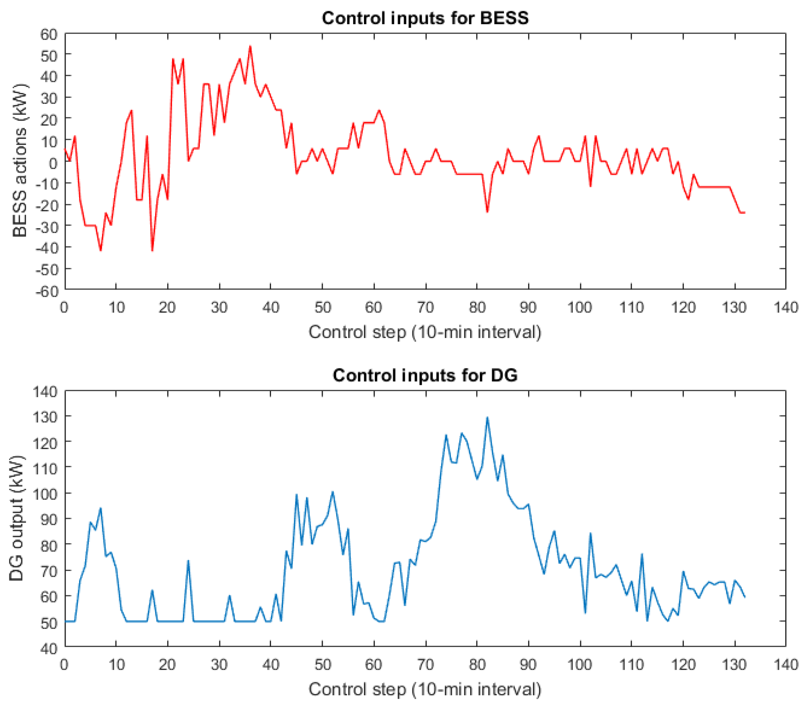
5.3. Simulation Results

The indoor temperature controlled with the variable structure controller is illustrated in Figure 5. We include a 0.2 per step time delay in the controller, which is 2 min in practice. With a set point temperature of 23 Celsius, the outdoor temperature and the corresponding indoor temperature over the first 50 control steps are shown in Figure 6. In addition, with an initial battery energy state of 120 kWh, the control inputs for the BESS and the DG solved with the proposed strategy are summarized in Figure 6. Based on the obtained results, one can observe that most of the charging actions are solved over the initial steps of the simulation where the temperature is relatively lower than other periods. As a result, the excess solar power would be charged into the BESS. In addition, the outdoor temperature gradually increases and reaches the peak at step 50, and the majority of the discharging actions of the BESS can be observed over this period. Once the energy stored in the BESS reaches a relatively lower state, the DG becomes the leading supplier to the TCLs afterward. The corresponding operational cost calculated with the simulation results is around 8606.98.

Since the rolling horizon approach is utilized, we record only the first components in the sets of BESS actions and the corresponding output power of DG. It should be pointed out that the forecasted PV and temperature data are used to compute these actions; while the system states are updated with the actual PV and temperature data using Equation (4). Furthermore, as the initial state is on 50% of the battery state-of-charge, there is no power curtailment during the one-day simulation.

5.4. Comparison Study

To evaluate the effectiveness of our algorithm, we compare it with the control scheme introduced in [9], in which a differential evolution (DE) algorithm is used. The DE algorithm is a population-based heuristics optimizer [22], and the choice of parameters in the algorithm, such as the population size, crossover rate, and mutation factor, could affect the optimization performance [23]. Therefore, this could increase the difficulty of implementing it in practice with the rolling horizon approach, as the microgrid operators are required to adjust those parameters for different sets of data. The DE algorithm can be used to solve the minimization problem $mi{n}_{x_1,\cdots x_n}f(x_1,x_2,\cdots ,x_n)$, where $x_i$ are the variables. The pseudocode of the DE algorithm [24] is described in Algorithm 1.

Algorithm 1 Differential evolution

1: procedure  2:     Step 0. Initialization:  3:     Number of variables n  4:     Population size NP mutation factor F, crossover rate CR  5:     Maximum iteration number, Maxiter  6:     Upper and lower bounds for all variables:  7:     $x_i^{min},x_i^{min},\forall i$.  8:     Step 1. Generate random initial population:  9:     for $i=1\mathit{to}NP$ do 10:         for $i=1\mathit{to}n$ do 11:            $x(i,j)=x_j^{min}+rand[0,1](x_j^{max}-x_j^{min})$ 12:         end for 13:     end for 14:     Step 2. Mutation and Crossover process: 15:     for $I=1\mathit{to}Maxiter$ do 16:         for $i=1\mathit{to}NP$ do 17:            $Selectrandom{r}_1,r_2,r_3\in [1,NP]$ 18:            $r_1\ne r_2\ne r_3\ne i$ 19:            $jrand=randInt[1:n]$ 20:            for $j=1\mathit{to}n$ do 21:                if $rand[0,1]<CRorj==jrand$ then 22:                    $V_{i,j}^{I+1}=x_{i,r1}^I+F(x_{i,r2}^I-x_{i,r3}^I)$ 23:                else 24:                    $V_{i,j}^{I+1}=x_{i,j}^I$ 25:                end if 26:            end for 27:         end for 28:         Step 3. Selection: 29:         if $f\left(v(I+1)\right)\le f\left(x_i\left(I\right)\right)$ then 30:            $x_i^{I+1}=v_{i,j}^{I+1}$ 31:         else 32:            $x_i^{I+1}=x_i^I$ 33:         end if 34:     end for 35: end procedure 36: $\mathit{End}$

In our case, the variables are control inputs for BESS. The mutation factor and crossover rate used in our simulation are both 0.9, and the maximum number of iteration is 50. Furthermore, we test the DE algorithm with the same simulation scenario considered in Section 5.2, and the results obtained with the population size of 60 is presented in Figure 7.

It should be pointed out that the results obtained with the DE algorithm are inconsistent, and we need to repeat the algorithm multiple times to achieve the best result. This could be undesirable for real-time scheduling. In our case, the corresponding operational cost over the one-day simulation is around 9527.65, which is much higher than the result solved with the proposed algorithm in this paper. Furthermore, we test the DE algorithm under different population sizes, and results are summarized in

Table 2. Cost of system units under different conditions.

	BESS Operation Cost ($)	DG Operation Cost ($)	Total
DE NP:60	8541.54	986.11	9527.65
DE NP:120	8389.07	1003.39	9392.46
DE NP:180	8209.49	814.89	9024.39
Proposed scheme	8181.21	425.76	8606.98

.

It can be perceived that the results can be improved at higher population sizes. By further increasing the population size, (e.g., up to 100 times of the variables) we could obtain results that are close to the one solved by the proposed scheme, but it would require multiple runs of the algorithm with adjustments on the parameters. In addition, it should be pointed out that the conditions to curtail the excessive energy are not considered in [9]. As a result, during our simulation, we found that with some sets of simulation data, such as a relatively low initial BESS state, the DE algorithm can generate results containing errors because the constraints set in the algorithm code cannot be satisfied. Since the model predictive control approach is used in our scheme, we believe that the dynamic programming algorithm will be a more appropriate choice as it does not require any adjustments in the code during the real-time operation. In addition, the actual level of reduction could be more significant if the unused energy stored in the BESS at the end of the process is considered.

5.5. Discussion

The proposed method can achieve better results than the one used for comparison. In consideration of the practical application, the proposed approach could be more reliable since the adjustment of parameters in the algorithm is unnecessary. Furthermore, the decentralized control scheme is critical to the real-time energy scheduling in the microgrid. Based on the previous sections, it can be perceived that the control of TCLs is only based on the indoor temperature in the corresponding area, and the operation of the generator and batteries are independent of the current measurements of indoor temperature. In order words, direct controls and communications between the central energy management system and the distributed TCLs are not required, which significantly improve the efficiency of the system, and the cost of constructing the whole system can be reduced.

6. Conclusions

A microgrid power scheduling strategy was introduced. The objective was to minimize the cost required to keep the room temperature under the desired level. A decentralized control scheme was proposed. The controller for each TCL needs to measure only indoor temperature in the corresponding area. The control input for the BESS charge/discharge does not need to have any measurements from TCL units, so the proposed system does not require any significant data communication subsystem. The conducted computer simulations showed that the proposed control scheme significantly outperforms other control algorithms. The proposed method is fully decentralized, computationally efficient and easily scalable. Moreover, the optimality of the proposed algorithm has been proved in a mathematically rigorous way.

In future studies, we will focus on determining an optimal BESS capacity for different scales of microgrids. To achieve that, we believe that an economic cost model of the BESS considering the degradation of batteries from actions under different conditions, such as temperature, depth of discharge, and rates of charge/discharge should be constructed. In addition, the long-term historical data on temperature and solar power should be investigated to determine the charge/discharge patterns over different seasons, and a possible objective function to determine the optimal capacity can be the minimization of power curtailments, battery lifetime consumption, and the unused BESS capacity over a period. Another important direction of future research is to test the proposed control algorithm in experiments with a real microgrid.

References

1. Khalid, M.; Ahmadi, A.; Savkin, A.V.; Agelidis, V.G. Minimizing the energy cost for microgrids integrated with renewable energy resources and conventional generation using controlled battery energy storage. Renew. Energy 2016, 97, 646–655. [Google Scholar] [CrossRef]
2. Wang, D.; Qiu, J.; Reedman, L.; Meng, K.; Lai, L.L. Two-stage energy management for networked microgrids with high renewable penetration. Appl. Energy 2018, 226, 39–48. [Google Scholar] [CrossRef]
3. Li, Y.; Yang, Z.; Li, G.; Zhao, D.; Tian, W. Optimal scheduling of an isolated microgrid with battery storage considering load and renewable generation uncertainties. IEEE Trans. Ind. Electron. 2019, 66, 1565–1575. [Google Scholar] [CrossRef]
4. Li, Y.; Yang, Z.; Li, G.; Mu, Y.; Zhao, D.; Chen, C.; Shen, B. Optimal scheduling of isolated microgrid with an electric vehicle battery swapping station in multi-stakeholder scenarios: A bi-level programming approach via real-time pricing. Appl. Energy 2018, 232, 54–68. [Google Scholar] [CrossRef] [Green Version]
5. Meng, K.; Wang, D.; Dong, Z.Y.; Gao, X.; Zheng, Y.; Wong, K.P. Distributed control of thermostatically controlled loads in distribution network with high penetration of solar PV. CSEE J. Power Energy Syst. 2017, 3, 53–62. [Google Scholar]
6. Kundu, S.; Sinitsyn, N.; Backhaus, S.; Hiskens, I. Modeling and control of thermostatically controlled loads. arXiv 2011, arXiv:1101.2157. [Google Scholar]
7. Bomela, W.; Zlotnik, A.; Li, J.S. A phase model approach for thermostatically controlled load demand response. Appl. Energy 2018, 228, 667–680. [Google Scholar] [CrossRef] [Green Version]
8. Wei, C.; Xu, J.; Liao, S.; Sun, Y.; Jiang, Y.; Zhang, Z. Coordination optimization of multiple thermostatically controlled load groups in distribution network with renewable energy. Appl. Energy 2018, 231, 456–467. [Google Scholar] [CrossRef]
9. Luo, F.; Xu, Z.; Meng, K.; Yang Dong, Z. Optimal operation scheduling for microgrid with high penetrations of solar power and thermostatically controlled loads. Sci. Technol. Built Environ. 2016, 22, 666–673. [Google Scholar] [CrossRef]
10. Zhou, Y.; Wang, C.; Wu, J.; Wang, J.; Cheng, M.; Li, G. Optimal scheduling of aggregated thermostatically controlled loads with renewable generation in the intraday electricity market. Appl. Energy 2017, 188, 456–465. [Google Scholar] [CrossRef]
11. Khalid, M.; Savkin, A.V. A model predictive control approach to the problem of wind power smoothing with controlled battery storage. Renew. Energy 2010, 35, 1520–1526. [Google Scholar] [CrossRef]
12. Khalid, M.; Aguilera, R.P.; Savkin, A.V.; Agelidis, V.G. A market-oriented wind power dispatch strategy using adaptive price thresholds and battery energy storage. Wind Energy 2018, 21, 242–254. [Google Scholar] [CrossRef]
13. Khalid, M.; Aguilera, R.P.; Savkin, A.V.; Agelidis, V.G. On maximizing profit of wind-battery supported power station based on wind power and energy price forecasting. Appl. Energy 2018, 211, 764–773. [Google Scholar] [CrossRef]
14. Khalid, M.; AlMuhaini, M.; Aguilera, R.P.; Savkin, A.V. Method for planning a wind–solar–battery hybrid power plant with optimal generation-demand matching. IET Renew. Power Gener. 2018, 12, 1800–1806. [Google Scholar] [CrossRef]
15. Khalid, M.; Savkin, A.V. An optimal operation of wind energy storage system for frequency control based on model predictive control. Renew. Energy 2012, 48, 127–132. [Google Scholar] [CrossRef]
16. Qiu, J.; Meng, K.; Zheng, Y.; Dong, Z.Y. Optimal scheduling of distributed energy resources as a virtual power plant in a transactive energy framework. IET Gener. Trans. Dis. 2017, 11, 3417–3427. [Google Scholar] [CrossRef]
17. Sideratos, G.; Hatziargyriou, N.D. An advanced statistical method for wind power forecasting. IEEE Trans. Power Syst. 2007, 22, 258–265. [Google Scholar] [CrossRef]
18. Khalid, M.; Savkin, A.V. A method for short-term wind power prediction with multiple observation points. IEEE Trans. Power Syst. 2012, 27, 579–586. [Google Scholar] [CrossRef]
19. Asrari, A.; Wu, T.X.; Ramos, B. A hybrid algorithm for short-term solar power prediction—Sunshine state case study. IEEE Trans. Sustain. Energy 2017, 8, 582–591. [Google Scholar] [CrossRef]
20. Bellman, R.E. Dynamic Programming; Princeton University Press: Princeton, NJ, USA, 2010. [Google Scholar]
21. Weatherzone. Sydney Observations. 2018. Available online: http://www.weatherzone.com.au/nsw/sydney/ (accessed on 20 October 2018).
22. Fleetwood, K. An Introduction to Differential Evolution. 2018. Available online: http://www.maths.uq.edu.au/MASCOS/Multi-Agent04/Fleetwood.pdf (accessed on 12 March 2019).
23. Ahlers, F.J. Differential Evolution (DE) for Conituous Function Optimization (an Algorithm by Kenneth Price and Rainer Storn). 2018. Available online: http://www1.icsi.berkeley.edu/~storn/code.html (accessed on 12 March 2019).
24. Cortés-Antonio, P.; Rangel-González, J.; Villa-Vargas, L.A.; Ramírez-Salinas, M.A.; Molina-Lozano, H.; Batyrshin, I. Design and implementation of differential evolution algorithm on FPGA for double-precision floating-point representation. Acta Polytech. Hung. 2014, 11, 139–153. [Google Scholar]
Figure 1. Configuration of the microgrid.
Energies 12 02111 g001
Figure 2. Flow chart of the proposed algorithm.
Energies 12 02111 g002
Figure 3. Actual and forecasted outdoor temperature.
Energies 12 02111 g003
Figure 4. Actual and predicted solar power.
Energies 12 02111 g004
Figure 5. Ambient and controlled indoor temperature.
Energies 12 02111 g005
Figure 6. Simulation results of battery energy storage system (BESS) action and distributed generator (DG) output.
Energies 12 02111 g006
Figure 7. Control inputs for BESS and DG solved with DE algorithm.
Energies 12 02111 g007