An Energy Management System for Residential Autonomous DC Microgrid Using Optimized Fuzzy Logic Controller Considering Economic Dispatch

Abstract

This work presents the operation of an autonomous direct current (DC) DC microgrid for residential house controlled by an energy management system based on low complexity fuzzy logic controller of only 25-rules to manage the power flow that supply house load demand. The microgrid consists of photovoltaic (PV), wind turbine, fuel cell, battery energy storage and diesel generator. The size of the battery energy storage is determined based on the battery sizing algorithm depending on the generation of renewables during all seasons of the year in the eastern region of Saudi Arabia. Two scenarios are considered in this work. In the first scenario: the microgrid consists of solar PV, wind turbine, battery energy storage and fuel cell. The fuzzy logic controller is optimized using an artificial bee colony technique in order to increase the system energy saving efficiency and to reduce the cost. In the second scenario: wind turbine is replaced by a diesel generator, also the rated power of the fuel cell is reduced. In this scenario, a new method is proposed to reduce the generation cost of the dispatchable sources in the microgrid by considering economic dispatch within the optimized fuzzy logic energy management system. To obtain the most suitable technique for solving the economic dispatch problem, three optimization techniques were used which are particle swarm optimization, genetic algorithm and artificial bee colony based on real environmental data and real house load demand. A comparison in terms of energy saving between the two scenarios and a comparison in terms of cost reduction between conventional economic dispatch method and the proposed method are presented.

1. Introduction

Growing concerns about climate change caused by fossil fuel consumption have made renewable energy (RE) become one of the hottest research areas. Governments all over the world encourage their nations through specific policies and regulations to employ RE technologies. Currently, 67 countries around the world have their own RE targets to contribute to solving the global warming issues [1]. The past three years have recorded the most significant growth of RE around the world. RE is estimated to produce around 23.7% of the world electricity. This means that a quarter of the world’s electricity is generated from renewable resources whereas 77% of the new renewable installation was in favor of photovoltaic (PV) and wind turbine (WT) systems. Great effort is being conducted towards research on hybrid renewable resources systems that become known as microgrids. A microgrid is a system that integrates renewable resources in addition to one or more conventional power source to produce clean, sustainable, stable and reliable power [2]. It is highly recommended to include energy storage within the microgrid to improve its performance and stability. Microgrids can operate in both grid-connected and standalone modes. Several studies in the literature have been discussed the concept of microgrids [3,4].

Energy management system (EMS) is usually integrated within a microgrid due to the need for a control system to manage the operation of the intermittent renewable resources effectively [5]. Recently, several studies have been implemented fuzzy logic controller (FLC) to employ EMS on microgrids. Fuzzy logic shows an efficient control for microgrid especially when multi-functions are performed on the microgrid. In fact, FLC can deal with different tasks simultaneously and efficiently. It can also predict the wind velocity, sun radiation and load consumption or even the status of the grid. It is an efficient tool for dealing with multiple different tasks instead of having a precise model dealing with each task individually.

Fuzzy logic energy management system (FLEMS) is typically designed for microgrids to take a control action for specific purposes. Several studies in the literature implemented FLEMS in microgrids of different topologies to control the state of charge (SOC) of battery energy storage (BES) in order to increase their lifetime and offer smooth operation. For instance, the DC microgrid in Reference [6] consists of PV, WT and BES that supplies different types of loads controlled by FLEMS to extend the batteries lifetime by maintaining the SOC. The authors in Reference [7] developed a FLEMS for standalone microgrid consists of PV, WT, battery storage, and fuel cell (FC) in order to determine the FC electrolyzer and batteries power according to the batteries SOC and hydrogen tank level of the FC. The system is optimally capable to maintain the batteries lifetime and utilize their cost. A standalone AC/DC microgrid controlled by FLEMS consists of PV, WT and battery storage is presented in Reference [8]. The authors proposed a supervisory controller depending on FLC in order to operate the renewable resources efficiently, maintain battery SOC and manage the exchange power between the AC/DC microgrid. 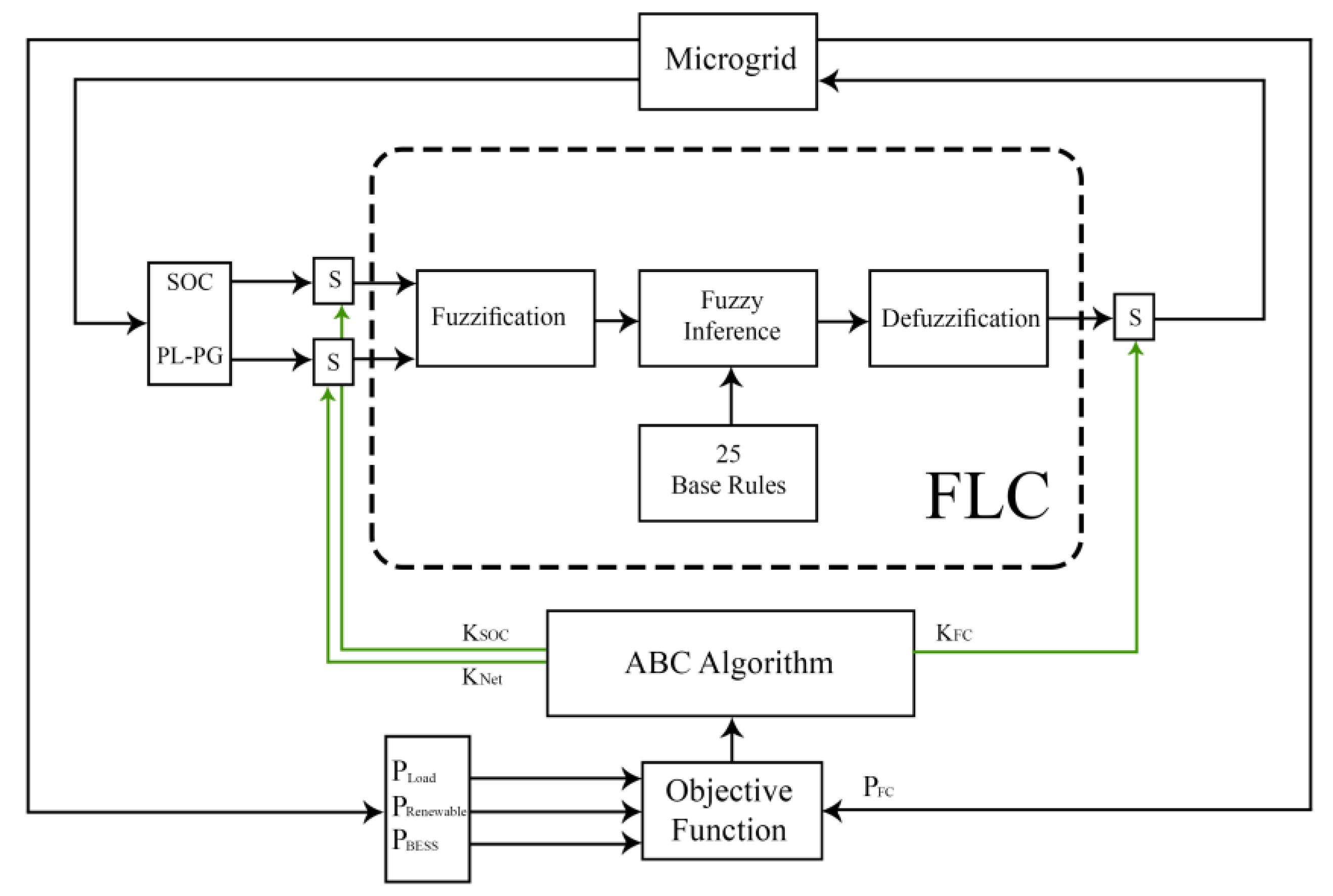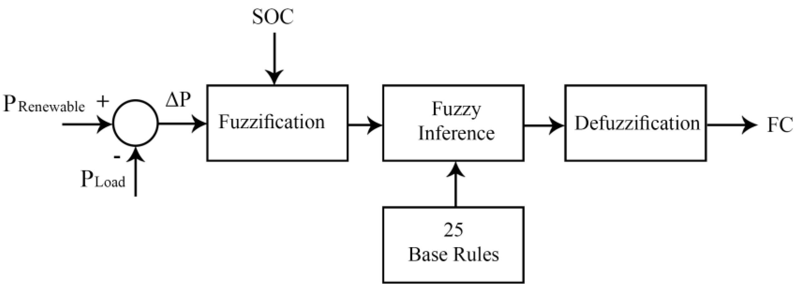A proposed FLEMS for grid-connected AC microgrid in Reference [9] smooths the grid power profile while maintaining the SOC of the BESS. The authors reached the lowest possible fuzzy logic rules (25 rules); hence, the system response was enhanced. The authors in Reference [10] proposed a FLEMS for AC microgrid that consists of PV, WT and FC of the type Proton-Exchange Membrane (PEMFC). The inputs of the controller are the frequency of the microgrid, batteries SOC, and the level of the water inside the water desalination tank. The control process is achieved by controlling the frequency of the main inverter. Efficiency in operation, reduction in size, and increases the batteries lifetime of the microgrid achieved by the proposed FLEMS. As we see from previous works, maintaining the SOC of battery storage is one of the fundamental aspects when designing the EMS of microgrids of different topologies.

Other control purposes of FLEMS for microgrids exist in the literature. Increasing the heat production and optimizing the economic dispatch to lower the generation cost are the main objectives of the microgrid system in Reference [11] that contains combined heat and power (CHP). The FLC in the work is used to account the uncertainty of electrical and thermal energy demands while other optimization techniques used to solve the economic dispatch problem. The authors in Reference [12] designed an FLEMS for a microgrid to maximize hydrogen production and optimize the microgrid power flow and generation. The microgrid in the work composed of PV, FC and BESS controlled by FLEMS. In the work in Reference [13], the FLEMS controls several processes in the microgrid such as load shedding and reduction of energy utilization cost as well as${\mathrm{CO}}_2$ emissions. The microgrid composed of PV model and battery storage. Last but not least, utilizing the heat generated for PV in water heating hence reduce power consumption as in Reference [14] and Controlling the duty cycle of maximum power point tracker (MPPT) for PV under different values of irradiance as in Reference [15].

Optimizing the FLEMS gives a higher degree of precise control, hence higher efficient operation, and lower cost of backup systems and more balanced operation between generation and consumption. A number of studies in literature optimized the FLEMS of microgrids. Different optimization techniques were used in the literature for optimizing microgrids FLEMS. Particle swarm optimization (PSO) is one of the famous intelligent techniques used for this purpose. The authors in Reference [16] proposed an EMS for microgrid using 49 rules of fractional order fuzzy PID and optimized using chaotic map adapted PSO algorithms. The system with optimized parameters shows an efficient and desirable suppression of microgrid frequency oscillation compared with the traditional controller. Another frequency controller for microgrid FLEMS was optimized in Reference [16]. Fuzzy logic membership functions of the system were tuned using the PSO technique and desired control level were obtained. The AC/DC hybrid microgrid in Reference [17] is controlled by FLEMS to maintain the SOC of the batteries of the two microgrids. The system configuration has been optimized using multi-objective PSO (MOPSO) to reduce the system cost and energy loses. Authors in Reference [18] proposed a battery charging control strategy based on FLC for a group of household microgrids that consist of 74 houses. PSO is used to optimize the membership functions of FLEMS. The optimized FLEMS can efficiently reduce the costs of battery charging of the houses during day hours. Other intelligent techniques are also used for optimizing the operation of microgrid FLEMS. Genetic algorithm (GA) optimization technique was used in Reference [19] for a microgrid that consists of WT, diesel generator, battery storage, and FC. the system uses two types of GA; one of them generates the day time scheduling management of the microgrid and the other on optimizes the FLEMS that controls the battery storage operation. A microgrid comprises hybrid micro-sources which are PV and FC, is proposed in Reference [20] to reduce the energy cost and ensure reliable energy supply giving the priority to the renewable resource. A modified seeker optimization approach (SOA) was used to tune the membership functions of the FLC in order to compute the gain factors of the dynamic proportional integral (DIP) controller. As noticed from the literature, there are many advantages achieved by utilizing intelligence techniques for optimizing FLEMS of different microgrid topologies.

Limited research has been conducted on optimizing FLEMS of microgrids using artificial bee colony (ABC) optimization technique. In Reference [21], a standalone microgrid that consisted of WT and DG used fuzzy logic based proportional integral derivative (FLPID) controller to control the diesel governor and the pitch angle of the WT. The authors employed ABC optimization technique to optimize 49 fuzzy rules as well as scaling factors. The authors in Reference [22] also used ABC to optimize the parameters of FLPID controller of a microgrid that has 49 fuzzy rules. The microgrid in the work consisted of a PV system, WT, DG and FC. The FLPID controlled the operation of the FC depending on active and reactive power fluctuations of the renewable generation.

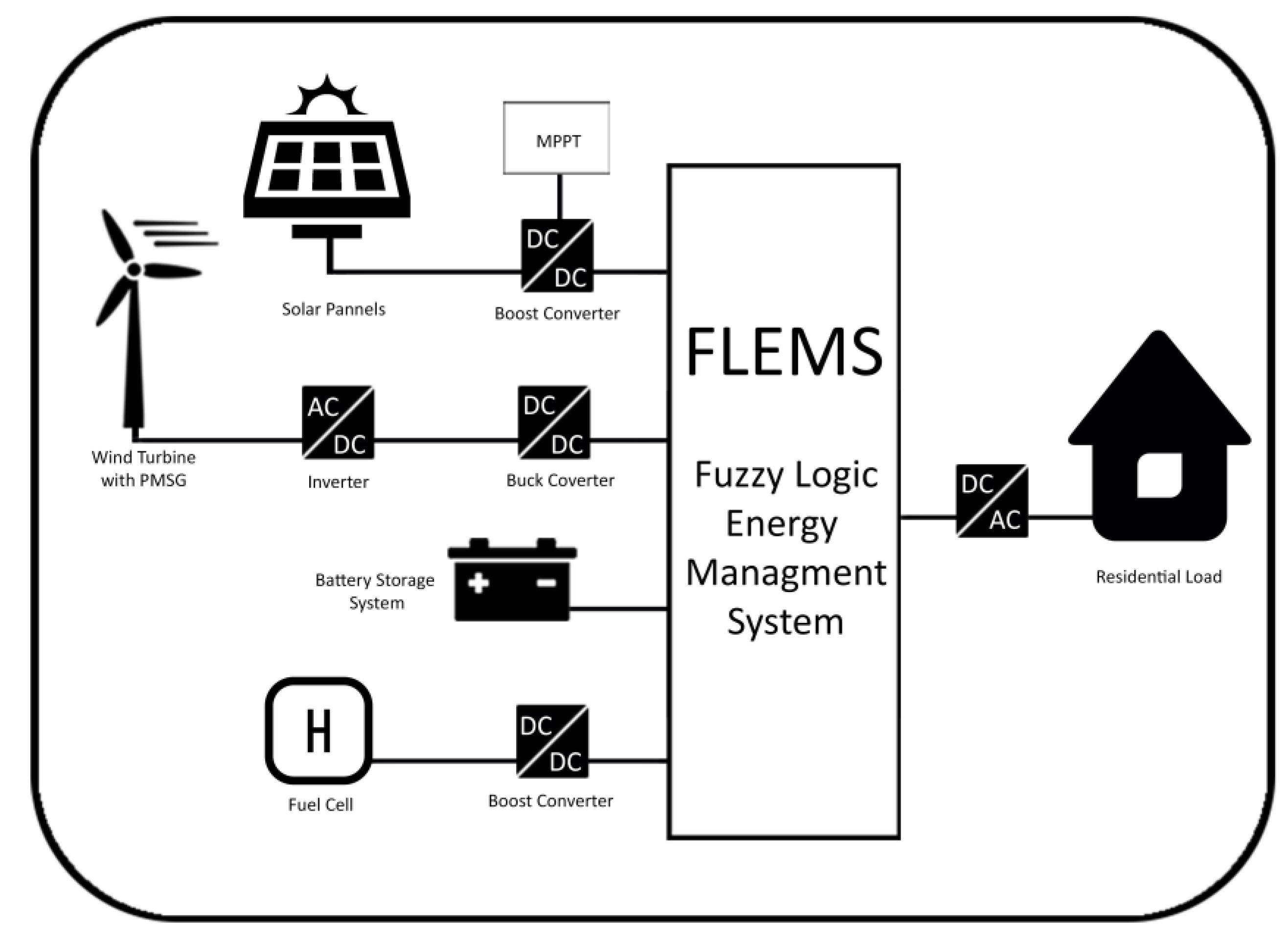
This paper presents the design, modeling, and operation of a DC microgrid controlled by an optimized and low complex FLEMS depending on real data collected from Dhahran city in Saudi Arabia. This work is divided into two main stages. In the first stage, the microgrid consists of PV, WT, FC and battery energy storage connected to load demand of a real house. The low complex FLEMS that has only 25 rules is optimized using ABC intelligent technique to enhance the system efficiency in terms of energy saving. The ABC algorithm obtains the optimal values of the scaling factors and membership functions of the FLC. In the second stage, the WT is excluded due to low wind speed in the given location and replaced by a diesel generator. A new approach is introduced by using an economic dispatch (ED) within the FLEMS to reduce the generation cost and increase the system efficiency. A comparison is presented between conventional ED and the proposed FLEMS considering ED.

To outline this paper, Section 2 describes the mathematical models of the microgrid components and its architecture in the first stage. Section 3 presents the design and optimization methodology of the FLEMS. Section 4 presents the configuration of the microgrid in the second stage and the methodology used to consider the ED within the FLEMS. Section 5 presents the simulation results of the microgrid operation in the two stages based on real environmental and load data. Section 6 concludes the paper.

2. Mathematical Model of the Microgrid

The components of the microgrid as shown in Figure 1 were built in MATLAB simulink environment based on their equivalent circuits and mathematical equations of each part. In addition, power electronic devices are used to integrate the components and form the microgrid such as buck/boost converters, MPPT and inverters that connected to the DC bus of the system. The following subsections present the mathematical models of each part in the microgrid.

2.1. Photovoltaic Solar Model

PV cells are the fundamental unit of the PV system. These cells aggregated in a series manner to form a module, and modules could be connected in series, parallel or even both to form what is known as an array.

Photovoltaic cells are the fundamental unit of the PV system. PV cells aggregated in a series manner to form a module. Modules can be connected in series, parallel or even both to form what is known as arrays. The ideal photovoltaic cell is represented mathematically by the following equation:

$$I= I_{pv}- I_0 \left[\exp \left(\frac{V+ R_{s}I}{V_{t}a}\right)- 1\right]- \frac{V+R_{s}I}{R_p}$$

(1)

where $I_{pv}$ and $I_0$ represent the PV and saturation currents of the array respectively, $V_t$ is the thermal voltage of the array and equals to $\left(NskT/q\right)$ where Ns is the number of cells connected in series, $q$ is the electron charge ($1.60217646\times {10}^{-19}$C), $k$ is the Boltzmann constant ($1.3806503\times {10}^{-19}$ J/K), $T$ is the ambient temperature in Kelvin, and V is the output voltage of the PV cell (greater output voltage obtained if cells connected in series while greater current obtained if cell connected in parallel), $a$ is the diode ideality constant, $R_s$ and $R_p$ are the equivalent series and parallel resistance of the array respectively as shown in the equivalent circuit of sing diode PV model in Figure 2.

The formula in Equation (1) is used for modeling a single panel or module that has low output power. To increase the output power to a certain level, the system should be modeled as a number of arrays compose several modules connected even in series, parallel or both. The light generated current of the PV cell depends linearly on the solar irradiation and affected by the temperature given as:

$$I= \left(I_{pv,n }+ K_I{\Delta }_T\right) \frac{G}{G_n}$$

(2)

where $I_{pv,n}$ is the light-generated current at nominal conditions (usually $25°$C and 1000 W/${\mathrm{m}}^2$) given in Ampere. $K_I$is the temperature coefficient of open circuit voltage ($V_{0c}).$ ${\Delta }_T$ = T – $T_n$ (T and $T_n$ being the actual and nominal temperatures) given in Kelvin. G is the irradiation on the device surface, and $G_n$ is the nominal irradiation given in [W/${\mathrm{m}}^2$]. $I_0$ is the diode saturation current, which is directly depending on the temperature, and it can be calculated as follows:

$$I_0=I_{0,n}{\left(\frac{T_n}{T}\right)}^{3}exp\left[\frac{q{E}_g}{ak}\right]\left(\frac{1}{T_n}-\frac{1}{T}\right)$$

(3)

where $E_g$ is the semiconductor bandgap energy and equals to $E_g$ ≈ 1.12 eV for the polycrystalline silicon at a temperature of $25°$C, $k$ is the Boltzmann constant, $I_{0,n}$ represents the nominal saturation current given by:

$$I_{0,n}=\frac{I_{sc,n}}{\exp \left(\frac{V_{0c,n}}{a{V}_{t,n}}\right)-1}$$

(4)

where $V_{t,n}$ being the thermal voltage of Ns cells connected in series at the nominal temperature$T_{n }$, $V=V_{0c,n}$, I = 0, and $I_{pv }$≈$I_{sc,n}$. In order to obtain a higher amount of power, a number of modules were connected in a parallel-series fashion. The module used in this work gives an amount of 5 kW rated power. For this approach, the equivalent circuit of a single diode PV cell, as illustrated in Figure 2, was constructed as showed in Figure 3 and formula in Equation (1) became

$$I= I_{pv}{N}_{par}- I_0{N}_{par} \left[exp\left(\frac{V+ R_s\left(\frac{N_{Ser}}{N_{par}}\right)I}{V_{t}a{N}_{Ser}}\right)- 1\right]- \frac{V+R_s\left(\frac{N_{Ser}}{N_{par}}\right)I}{R_p\left(\frac{N_{Ser}}{N_{par}}\right)}$$

(5)

where $N_{Ser}$ and $N_{par}$ are the numbers of series and parallel modules in an array and $N_S$ is the number of series cells in each individual module. The parameters of the PV model are set according to KC200GT array module that generates 200 W as rated power output at ideal conditions (ambient temperature at $25°$C and irradiation at 1000 W/${\mathrm{m}}^2$) [23,24,25,26].

2.2. Wind Turbine Model

Wind energy; one of the most abundant resources, is the second fastest growing RE technology worldwide. The wind turbine generators are evolving rapidly in two directions; technically and industrially. WT system consists of three main parts forming the system that converts the wind energy into electricity. The first part is the rotor and it has three fiberglass blades. They are included within a hub that has a hydraulic motor, which has the ability to change the blades directions in order to operate efficiently with variable wind speeds. The nacelle behind the turbine contains the shaft and gearbox that increases the speed. In addition, it contains the transformer and the generator. The third part is the tower that supports the previous two parts. WT integrated with permanent magnet synchronous generator (PMSG) became more popular due to its efficiency when experiencing low wind speed. Several studies in the literature included a model of a wind turbine using PMSG [27,28,29]. The power generated by the wind turbine is given by:

$$P_w=0.5\rho A{V}^3{C}_P\left(\lambda ,\theta \right)$$

(6)

where $P_w$ is the power comes from WT, A is the cross-section area of the blades of the WT given in m², $\rho$ is gas density available in the atmosphere, $C_P$ is the WT energy conversion coefficient, and V is the wind velocity given in (m/s). The energy conversion coefficient $C_P$ and the gas density $\rho$ are given as:

$$\rho =0.5A\left(\frac{353.05}{T}\right) ex{p}^{-0.034\left(\frac{z}{T}\right)}$$

(7)

$$C_P\left(\lambda ,\theta \right)= \left(\frac{116}{{\lambda }_i}-0.4\ast \theta -5\right)\mathrm{.0.5} ex{p}^{\frac{-16.5}{{\lambda }_i}}$$

(8)

where Z is the altitude, T is the ambient temperature, ${\lambda }_i$ is the tip speed ratio. $\theta$ represents the angle of the blades tilt. Formula (9) expresses the tip speed ratio and (10) expresses the initial tip speed:

$${\lambda }_i= \frac{1}{1/\left(\lambda +0.089\theta \right)-0.035/\left({\theta }^3+1\right)}$$

(9)

$$\lambda =r\frac{\omega R}{V}$$

(10)

where $\omega$ is the rotor rotational speed in radians/second, R is the rotor radius in meters, and V is the wind speed specified in meter/second.

2.3. Fuel Cell Model

A fuel cell is considered as an electrochemical system that can convert the chemical energy into electrical energy and produces heat and water as secondary products. It composes of a pair of electrolytes and electrode. Its structure seems like a battery with a difference that it can deliver power as long as it supplied by fuel. There are five types of fuel cells depending on the material used in the electrolyte: polymer electrolyte membrane fuel cell (PEMFC), phosphoric acid fuel cell (PAFC), solid oxide fuel cell (SOFC), alkaline fuel cell (AFC) and molten carbonate fuel cell (MCFC). Among these five types, PEMFC considered as the best due to its rapid development, simple structure, low operating temperature, quick start and high efficiency. It has two electrodes in each side with the electrolyte layer in the middle. Fuel, hydrogen and oxygen, is fed to the anode and cathode electrode respectively [30]. The output voltage of the fuel cell is given by:

$$E=E_n-(-V_{act}+V_{ohm}+V_{con)}$$

(11)

where $E_n$ is the Nernst voltage, $V_{act}$, $V_{ohm}$ and $V_{con}$ are the activation, ohmic and concentration voltages respectively. Each one of these losses is calculated as listed in (12)–(15):

$$V_{act}=-\left[{\xi }_1+{\xi }_2.T+{\xi }_3.T.ln\left(C_{O_2}\right)+{\xi }_4.T.ln\left(i_f\right)\right]$$

(12)

$$V_{ohm}=i_f.R_M$$

(13)

$$R_M=\frac{181.6[1+0.03\left(i_f/A_f\right)+0.062{\left(T/303\right)}^2{\left(i_f/A_f\right)}^{2.5}}{[{\lambda }_1-0.634-3\left(i_f/A_f\right)\left]- exp\right[4.18\left(\left(T-303\right)/T\right]} . \frac{l_1}{A_f}$$

(14)

$$V_{con}=-B_0.ln\left(1-\frac{J}{J_{max}}\right)$$

(15)

where $T$ is the absolute operating temperature, $C_{O_2}$ represents the concentration of oxygen, $i_f$ represents the fuel cell output current, $R_M$ is the resistance of membrane, $A_f$ represents the effective area, $l_1$ is the effective thickness of the membrane, ${\xi }_1,{\xi }_2,{\xi }_3,{\xi }_4$ are the reference coefficients, $B_0$ represents the operating constant. $J$ and $J_{max}$ are the current and maximum current density respectively.

2.4. Battery Energy Storage

Batteries are one of the most efficacious storage devices. They can store energy in electrochemical form. They can store energy from both DC and AC sources for future usage. Batteries are needed as a basic part of the microgrid. They discharge their energy to supply the loads whenever the microgrid resources are unable to meet the load demand or whenever one of the resources or more goes out of service. On the other hand, they charge with energy when the microgrid generation overcomes the load demand. Lithium-ion and lead-acid batteries are widely used for small electrical systems due to their special characteristics such as superior usable capacity, extended life cycle, small size, weight and climate resistances among other types. The discharging and charging expressions for BESS are given in (16) and (17) respectively

$$f_1\left(it i^{*}i\right)=E_0-K.\frac{Q}{Q-it}\left(i^{*}-it\right)+A.\exp \left(-B.it\right)$$

(16)

$$f_2\left(it i^{*}i\right)=E_0-K\left(\frac{Q}{it+0.1.Q}.i^{*}-\frac{Q}{Q-it}.it\right)+A.\exp \left(-B.it\right)$$

(17)

where $E_0$ represents the initial voltage, A is the exponential voltage given in (Volt), $i$ represents the battery current, $i^{*}$ represents the low-frequency dynamic current given in (Ampere), K represents the polarization resistance, Q related to the maximum capacity of the battery, it is the extraction capacity of the battery given in (Ah) and B represents the exponential capacity given in ${\left(\mathrm{Ah}\right)}^{-1}$. One of the most important parameters of BES is the state-of-charge which calculated as:

$$SOC=100\left(1-\frac{{{\displaystyle \int }}_0^{t}idt}{Q}\right)$$

(18)

where $i$ represents the battery current and Q related to the maximum capacity of the battery.

Battery Sizing

To determine the suitable and optimal size capacity of the battery storage system, one of the recent and effective algorithms named battery sizing algorithm (BSA) is used in this work. The idea behind this algorithm is to find an optimal size for the BES of the microgrid depending on the difference between the renewable systems generation and load demand [31]. The total generation of the renewable systems calculated according to:

$$P{G}_{Renewable,t}=P{G}_{solar,t}+P{G}_{wind,t}$$

(19)

where $P{G}_{solar,t}$ is the power generated from PV solar system and $P{G}_{wind,t}$ is the power generated from the WT system at time t respectively. The difference between the generation and the load demand is calculated as:

$$P_{Difference,t}=P{G}_{Renewable,t}- P{L}_{demand,t}$$

(20)

where $P{L}_{demand,t}$ is the power load demand. The first stage is allocated for finding the maximum storage size according to the excess power from the difference between generation and load demand:

$$BE{S}_{max}=min({\displaystyle \sum }_{t=1}^T{P}_{Difference,t})$$

(21)

where $BE{S}_{max}$ is the maximum capacity size of the BES. The second stage is allocated to find the required capacity of the battery which should not be the maximum all the time. The required capacity of BES is found according to:

$$BE{S}_{Cap}= \{\begin{array}{ll}BE{S}_{max},& x=1\\ CBS,& x=0\end{array}$$

(22)

where $BE{S}_{Cap}$ is the required capacity of the BES during all time and $CBS$ is the corrected battery size. The condition$x=1$ denotes that the BES is fully discharged after charging and the condition$x=0$ denotes that the BES is not fully discharged after the charging process and the battery capacity is oversized. Region reduction iterative algorithm is used to calculate the corrected BES size ($CBS$). The third stage of the algorithm is to find the optimal capacity size of the BES and calculated according to the given in the following formula:

$$BE{S}_{opt}= \{\begin{array}{ll}BE{S}_{cap},& BE{S}_{DV}\ge BE{S}_{lim} \\ BCS,& otherwise\end{array}$$

(23)

where $BE{S}_{opt}$ is the optimal capacity size of the BES, $BE{S}_{lim}$minimum battery utilization limit, $BE{S}_{DV}$ is the battery decision variable and calculated as stated in the literature. $BCS$ is the BES corrected size for the third stage and calculated using region reduction iterative algorithm. In order to find the optimal size of the battery storage system for the microgrid in this work, average generation from PV system and WT system for one year used in the BSA depending on real data such as irradiation, ambient temperature and wind speed. In addition, a real load demand recorded from a residential house in the same year is also used in the algorithm.

3. Fuzzy Logic Energy Management System of the Microgrid

The components of the microgrid in this work are integrated using power electronics devices and modeled using MATLAB/Simulink environment. The energy management system of the proposed microgrid as shown in Figure 1 is designed using FLC. In this work, FLEMS is designed with minimum possible fuzzy rules to reduce the complexity and enhance the control response of the proposed standalone DC microgrid.

3.1. Microgrid Specification

The following points summarize the specification of the proposed system:

• The photovoltaic solar system of 5 kW connected to power electronics such as DC/DC boost converter to meet the microgrid requirement. Maximum power point tracker is integrated with the converter to enable the PV system harvesting maximum power regardless of the variations in temperature and irradiation.
• The wind turbine system of 5 kW connected to power electronics such as AC/DC inverter to invert the AC output of the wind turbine into DC. In addition, the DC/DC buck converter used to step down the voltage and meet DC bus requirements of the microgrid. Parameters of the PMSG are the same as used in the literature mentioned in Section 2.2.
• The fuel cell of the type (PEMFC) (5 kW-45 V) connected to DC/DC converter to meet the DC bus requirements of the microgrid.
• Battery energy storage of 20 kWh capacity of the type Lead Acid. The size of the battery is obtained based on BSA that explained extensively in Section 2.4.
• House load demand modeled based on real data recorded from real house inside KFUPM campus. (House No. 3307 based HVAC VFD system).
• 110-volt DC bus collects the power from generation and backup sources according to the control actions of the FLEMS and supplies the load demand.

3.2. Fuzzy Logic Controller of the Energy management system

Figure 4 illustrates the fuzzy logic controller of the energy management system for the proposed microgrid. The FLC has two input variables, which are SOC of BES and the power difference.

ΔP represents the power difference between generated power from renewables and load demand power during day hours. It is calculated as:

$$\Delta p=P_{Renewable}-P_{load}$$

(24)

$$P_{Renewable }= P_{PV}+P_{WT}$$

(25)

where $P_{Renewable}$ is the power generated from renewables, $P_{load}$ is the power of the house load, $P_{PV}$ is the photovoltaic system power, and $P_{WT}$ represents the wind turbine power.

The output of the FLC controls the operation of FC to compensate for the absence of RE generation (REG) that comes from PV and WT when SOC of BES is at a minimum level. The BES is working within the limits between (20–95%) of its SOC.

Table 1. Fuzzy rules of the microgrid Fuzzy Logic Energy Management System (FLEMS).

FC Power		$\mathbf{\Delta }\mathit{P}({\mathit{P}}_{\mathit{R}\mathit{e}\mathit{n}\mathit{e}\mathit{w}\mathit{a}\mathit{b}\mathit{l}\mathit{e} }- {\mathit{P}}_{\mathit{l}\mathit{o}\mathit{a}\mathit{d}})$
		BN	SN	ZE	SP	BP
SOC	VL	VH	H	L	L	VL
	L	H	M	VL	VL	VL
	M	VL	VL	VL	VL	VL
	H	VL	VL	VL	VL	VL
	VH	VL	VL	VL	VL	VL

presents the 25 fuzzy rules of the proposed system. The abbreviations VL, L, M, H, VH stand for: very low, low, medium, high and very high respectively and the abbreviations BN, SN, ZE, SP, BP stand for big negative, small negative, zero, small positive and big positive respectively. For example, the output variable of the FLC is VH (the amount of the power supplied by FC is very high) when the input variable ΔP is BN (the amount of the load demand is very high, and the REG is very small) and the input SOC is VL (the stored energy the BES is very low). However, the output is VL when the input variable ΔP is ZE (the amount of load demand is equal to the REG) and the input variable SOC is M (the stored energy the BES is medium). The output variable is VL instead of M when the FLEMS works in the previous conditions because the microgrid renewable is generating enough power for the load demand and the BES still has energy for discharging. Thus, the FLC rules table is not symmetrical.

3.3. Optimization of FLEMS Using Artificial Bee Colony

The optimization in this work is done to enhance the output of the FLC to reach the desired action with good performance and high energy saving efficiency. The FLC controls the operation of backup systems in the microgrid (FC in this stage) during insufficient or absence of REG and BES. However, making the backup system following the varying load demand by minimum possible fuzzy rules is a difficult process. Therefore, optimizing the FLC using intelligent technique can make a difference in the microgrid control. ABC is one of the recent and effective intelligent optimization techniques. It is considered as an evolutionary algorithm. This technique simulates the foraging behavior of honeybees and has been used successfully in many applications. It was first proposed in 2005 by Karaboaga [32]. The artificial bee colony algorithm is divided into two halves that represent the two stages of the honeybee’s behavior. The first half allocated for the behavior of the employed bees and unemployed bees. The second half contains two types of bees: scout bees and onlooker bees. The first stage of the algorithm initializes the initial solutions $S_i$ (food sources) in a randomly distributed manner in N-dimensional vectors ($i=1, 2, 3,\dots , FN$) where N is the number of optimized parameters and $FN$ is the food sources number. After that, these were solutions subjected to a number of iterations in the complete search procedure. The employed bees start exploiting these sources, evaluate its quality according to the fitness function, and then share the information with onlooker bees. Depending on the probability value of the food source, onlooker bees chose a source of food. The onlooker bees calculate the probability value as:

$$P_n=\frac{S_{fitness,n}}{{{\displaystyle \sum }}_{i=1}^{FN}{S}_{fitness,i}}$$

(26)

where $P_n$ is the probability value of the desired source, $S_{fitness,n}$ is the current fitness source. After that, ABC produces a candidate food source from the old one in memory as:

$$V_{i,j}=x_{i,j}+{\varphi }_{i,j}\left(x_{i,j}-x_{k,j}\right)$$

(27)

where V represents the position of the new food source, x is the old food source position, $k=1,2,3,\dots ,FN$, $j=1,2,3,\dots ,N$ and $i=1,2,3,\dots ,N$ are random indexes, k must be different from i value and ${\varphi }_{i,j}$ is a random constant between [−1,1]. If the position source cannot be improved, the source is abandoned, and employed bees become scout bees and search for a new food source. The operation is defined as:

$$x_i^j=x_{min}^j+rand\left(0,1\right)\left(x_{max}^j-x_{min}^j\right)$$

(28)

where $x_i$ is the abandoned sources and $j\in \left\{1, 2, 3,\dots ,N\right\}$. The procedure repeats according to the iteration number until the best solution obtained [33].

Figure 5 illustrates the ABC algorithm flowchart and shows the steps of ABC optimization. The ABC algorithm searches for the optimal values of the scaling factors as well as the membership function values which are considered as “food sources” for the employed bees. The algorithm tries to find optimal solutions (food sources) according to the constraints and depending on the input variables. The input variables of the ABC algorithm are the load demand of the residential house, the power generated by REG, the amount of energy stored in the BES, and the power generated from FC controlled by the FLC. The objective of the algorithm is to reach an optimal amount of generation from the backup system which is FC in this stage giving the priority to the REG and BES to supply the load demand respectively. Figure 6 illustrates the optimization process for FLC.

The objective function of the optimization tends to minimize the error between the current operation of FC and actual power needed to be supplied from it. It can be written as:

$$f={{\displaystyle \int }}_0^T{\left|\Delta e\right|}^{2}dt$$

(29)

where $T$ is the simulation time (24 h) and $\Delta e$ is the error between generated power from FC and reference power. It is calculated as:

$$\Delta P=P_{Ref}-P_{FC}$$

(30)

where $P_{FC}$ is the fuel cell power and $P_{Ref}$ represents the reference power and it’s given as:

$$P_{Ref}=\{\begin{array}{ll}{P}_{Load}- P_{Renewable}- P_{BES},& P_{Load}\ge P_{\begin{array}{c}Renewable\\ \end{array}}\\ 0,& otherwisw\end{array}$$

(31)

where $P_{BES}$ is the power stored in the battery energy storage. Equations (11)–(14) represent the constraints of the objective function.

$$K_{Soc}^{min}\le K_{SOC}\le K_{Soc}^{max}$$

(32)

$$K_{NetPower}^{min}\le K_{NetPower}\le K_{NetPower}^{max}$$

(33)

$$K_{FCPower}^{min}\le K_{FCPower}\le K_{FCPower}^{max}$$

(34)

$$N_{MF Point}^{min}\le N_{MFpoint}\le N_{MF Point}^{max}$$

(35)

were $K_{SOC}$, $K_{NetPower}$ and $K_{FCPower}$ are the scaling factors of the two inputs and output of the FLC. $N_{MFpoint}$ is the value of each base of each membership function, thus each input and output of the FLC in this work has 10 base values. The minimum and maximum boundaries of these constants are initially determined by trial and error method.

4. FLEMS Considering Economic Dispatch

Due to low wind speed in Dhahran, the generation of small-scale WT for residential use will be less efficient. In addition to that, the installation cost of the WT is more expensive. Hence, from an economic point of view, it will be better if the WT is replaced by another source such as a diesel generator in this stage.

Unlike WTs, DGs are dispatchable sources since their rated power can be controlled according to the load demand. In this work, the microgrid has already a dispatchable source which is a fuel cell. Hence, to reduce the generation cost for these sources, the economic dispatch problem is solved and will be integrated with the FLEMS.

Economic dispatch is an expression uses for describing the optimal generation of several generators in an electrical system to meet the load demand while maintaining the lower possible cost of generation subjected to several constraints [34]. The economic dispatch problem usually solved using a special software program. Recently, optimization techniques are used, and they are gaining wide popularity.

The following points summarize the specification of the proposed system in this stage:

• Dispatchable backup sources of the microgrid in this stage are fuel cell and diesel generator.
• The size of the diesel generator is 1 KW and the size of the fuel cell is 3 kW, together they can deliver up to 4 kW during operation.

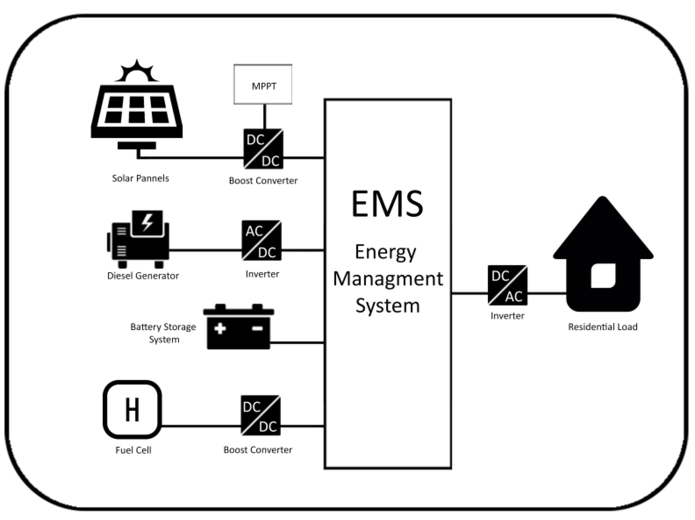
Figure 7 illustrates the microgrid configuration in this stage, where the wind turbine was replaced by a diesel generator. The aim of applying economic dispatch within the optimized FLEMS of the microgrid is to minimize the total generation cost. Hence, the optimized FLEMS that has been obtained from the first stage, using the ABC algorithm, is used in this stage. However, a further degree of optimization is introduced in this stage to optimize the FLEMS control for backup sources which are FC and DG using economic dispatch for cost reduction purpose. The idea is to set a specific limit for power generation for each hour of the day according to the economic dispatch solution. In addition to FLC control action, this assures a precise control for the operation of backup sources during insufficient generation of the RE resource. Hence, the generation cost is reduced. In order to develop the microgrid cost function, the cost function of each dispatchable source must be determined.

The cost function of DG is assumed as a second-order polynomial function as:

$$F_t\left(P_{DG,t}\right)=a_{DG}+b_{DG}{P}_{DG,t}+c_{DG}{P}_{DG,t}{}^2$$

(36)

where $F_t$ is the cost function of the diesel generator at time $t$. $\left(P_{DG,t}\right)$ is the output power of the diesel generator at the same time. $a_{DG}$, $b_{DG}$ and $c_{DG}$ are the cost coefficients of the DG. The cost function of the fuel cell is also assumed as a second-order polynomial function as:

$$F_t\left(P_{FC,t}\right)=a_{FC}+b_{FC}{P}_{FC,t}+c_{FC}{P}_{FC,t}{}^2$$

(37)

where $F_t$ is the cost function of the FC at time $t$. $\left(P_{FC,t}\right)$ is the output power of the fuel cell at the same time. $a_{FC}$, $b_{FC}$ and $c_{FC}$ are the cost coefficients of the FC. Hence, the objective function can be written as follows:

$$Min.C={\displaystyle \sum }_{t=1}^T\left[F_t\left(P_{DG}\right)+F_t\left(P_{FC}\right)\right]$$

(38)

where $C$ is Total generation cost, $F_t\left(P_{DG}\right)$ is the cost function of the diesel generator at time t and $F_t\left(P_{FC}\right)$ is the cost function of the fuel cell at time t. The constraints are stated as follows; Equation (39) represents the equality constraint while Equations (40) and (41) represent the inequality constraints. The formula in Equation (39) implies that the EMS gives the priority to the REG to supply the load demand, if REG cannot supply enough power to the load then it takes power from BES. The lowest priority for supplying the load is given to the backup sources which FC and DG to minimize the generation cost.

$$P_{DG,t}+ P_{FC,t}= P_{Load,t}- P_{renewable,t}-P_{BES,t}$$

(39)

$$P_{DG}{}^{min}\le P_{DG}\le P_{DG}{}^{max}$$

(40)

$$P_{FC}{}^{min}\le P_{FC}\le P_{FC}{}^{max}.$$

(41)

The maximum and minimum boundaries of the inequality constraints are set depending on the rated power of DG and FC as:

$$0\le P_{DG}\le 1K$$

(42)

$$0\le P_{FC}\le 3KW.$$

(43)

The cost coefficients of the FC and the DG are set according to the literature [35,36] are shown in

Table 2. Cost coefficients of the dispatchable sources of the microgrid.

Coefficient	Fuel Cell	Diesel Generator
$a$	19.36	10
$b$	4.94	200
$c$	0.77	100

.

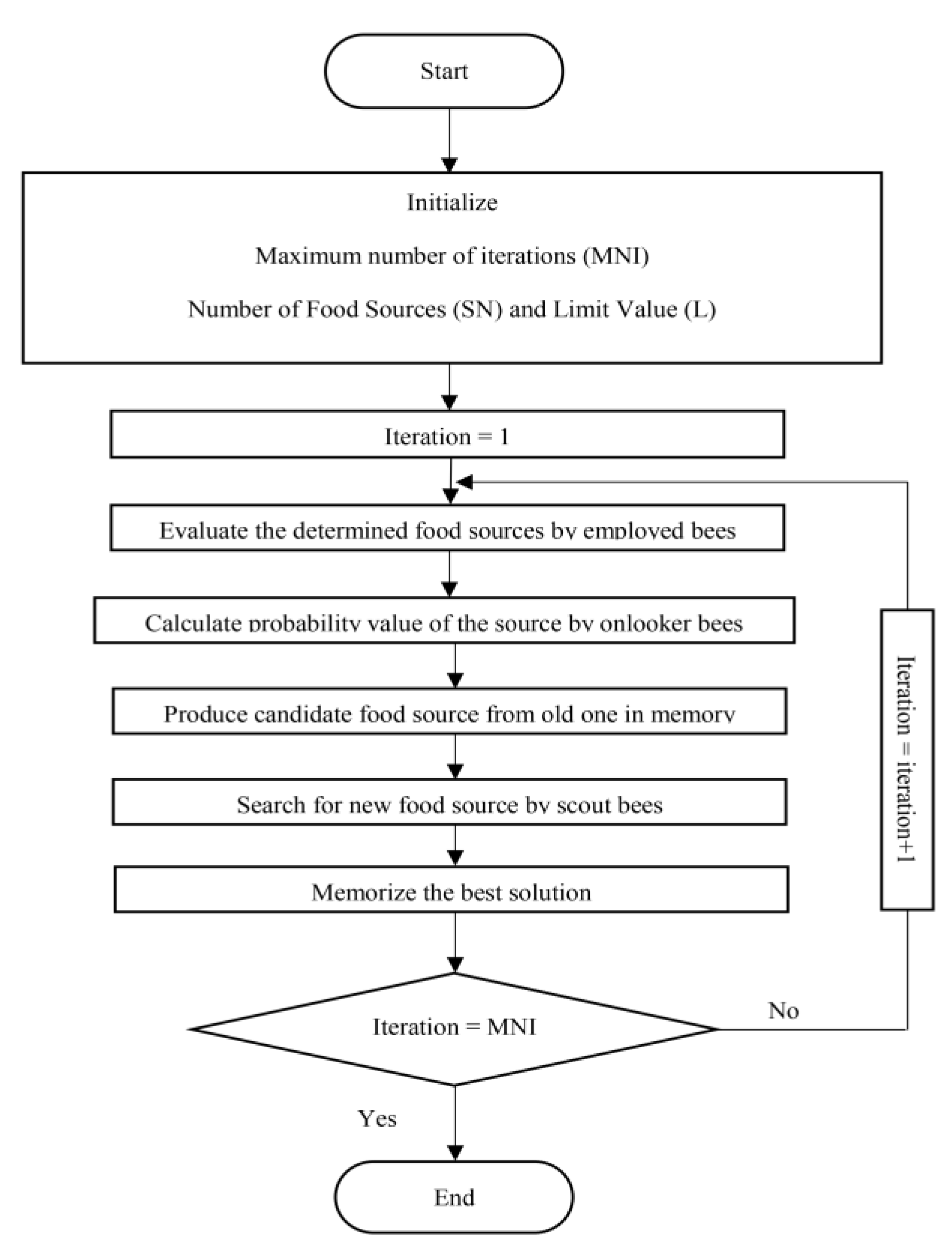
Three intelligent optimization techniques were conducted to solve the problem. One of them is ABC which was explained previously for optimizing the FLC. The other two techniques are PSO [37,38] and GA [39,40]. The aim of the economic dispatch problem for any power system that contains several dispatchable sources is solved to minimize the generation cost. The economic dispatch gives an optimal amount of power that each generator must produce in a specific time to operate the system economically. It is considered as a controlling approach that depends on the scheduling procedure. However, in this work, a new approach is proposed to control the dispatchable sources in the microgrid using economic dispatch within the optimized FLEMS.

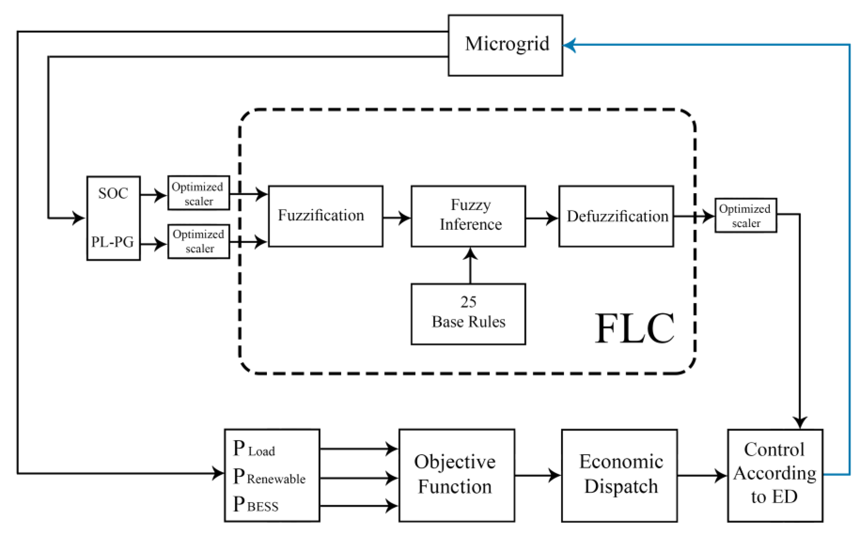
The idea behind this approach is to set a limit value of power generation for each dispatchable source in the microgrid system that controlled by the optimized FLEMS in each hour of the day. Figure 8 illustrates the proposed controlling process. The obtained limits of power generation for each hour of the day for each dispatchable source in the microgrid is embedded within the optimized FLEMS. The simulation results of the proposed method are compared with other methods results of the first stage. Comparison in terms of energy saving efficiency and generation cost is conducted among microgrid with unoptimized FLEMS, microgrid with optimized FLEMS, and microgrid with optimized FLEMS considering economic dispatch.

5. Results and Discussions

The simulation of this work is divided into two main stages as explained earlier. All microgrid components and power electronics used for integrating the components to form the microgrid are built using MATLAB/Simulink environment while the intelligent techniques used for optimization purpose is performed using MATLAB coding and connected to the microgrid in the Simulink.

The first subsection exhibits the simulation results of the microgrid operation controlled low complexity fuzzy logic energy management system before and after optimization. The results are optimized using artificial optimization technique while maintaining the minimum possible number of fuzzy rules. Real data of a hot summer day in Dhahran city used in simulation as a case of study. A comparison in terms of system energy saving efficiency before and after optimization is also presented.

The second subsection presents the simulation results of the solved economic dispatch problem using three intelligent optimization techniques to lower the operation cost and enhance the microgrid energy saving efficiency. In addition, the simulation results of the microgrid controlled by optimized FLEMS considering the economic dispatch are presented using real data for 24 hours of the same summer day as a case of study. A comparison in terms of efficiency and cost with conventional methods are also presented.

5.1. Microgrid FLEMS Optimization Using ABC Technique

In this stage, the proposed microgrid consists of 5 kW PV, 5 kW WT, 200 AH battery storage and 5 kW FC. The microgrid is connected to variable load house the has a maximum peak of 5 kW. The size of the RES is the rated generated power in ideal weather conditions; 1000 W/${\mathrm{m}}^2$for irradiation, $25°$C for ambient temperature, and 10 m/s for wind speed. However, this is not the usual case. For instance, in some days or some hours of the day, the REG becomes zero and the BES is at its lowest level; when no sun irradiation at night and wind speed is low or zero. Therefore, the backup systems compensate for the absence of these sources and supply the load demand. The size of the battery storage is determined according to a developed battery sizing algorithm (BSA). This algorithm uses the average output power from the PV and WT and the house load demand of all year days in the given location. All microgrid components are integrated together using power electronics devices controlled by FLEMS. Optimization using ABC algorithm is conducted to enhance the performance of the FLC that controls the operation of the fuel cell as a backup source. The optimization process is conducted for both; the membership functions and the scaling factors of inputs and output of the FLC of the microgrid. The system tested using real data of Dhahran city; 28th of July 2016, using solar irradiation, ambient temperature, wind speed and residential load demand recorded inside KFUPM campus. Comparison in system efficiency with/without optimization is presented.

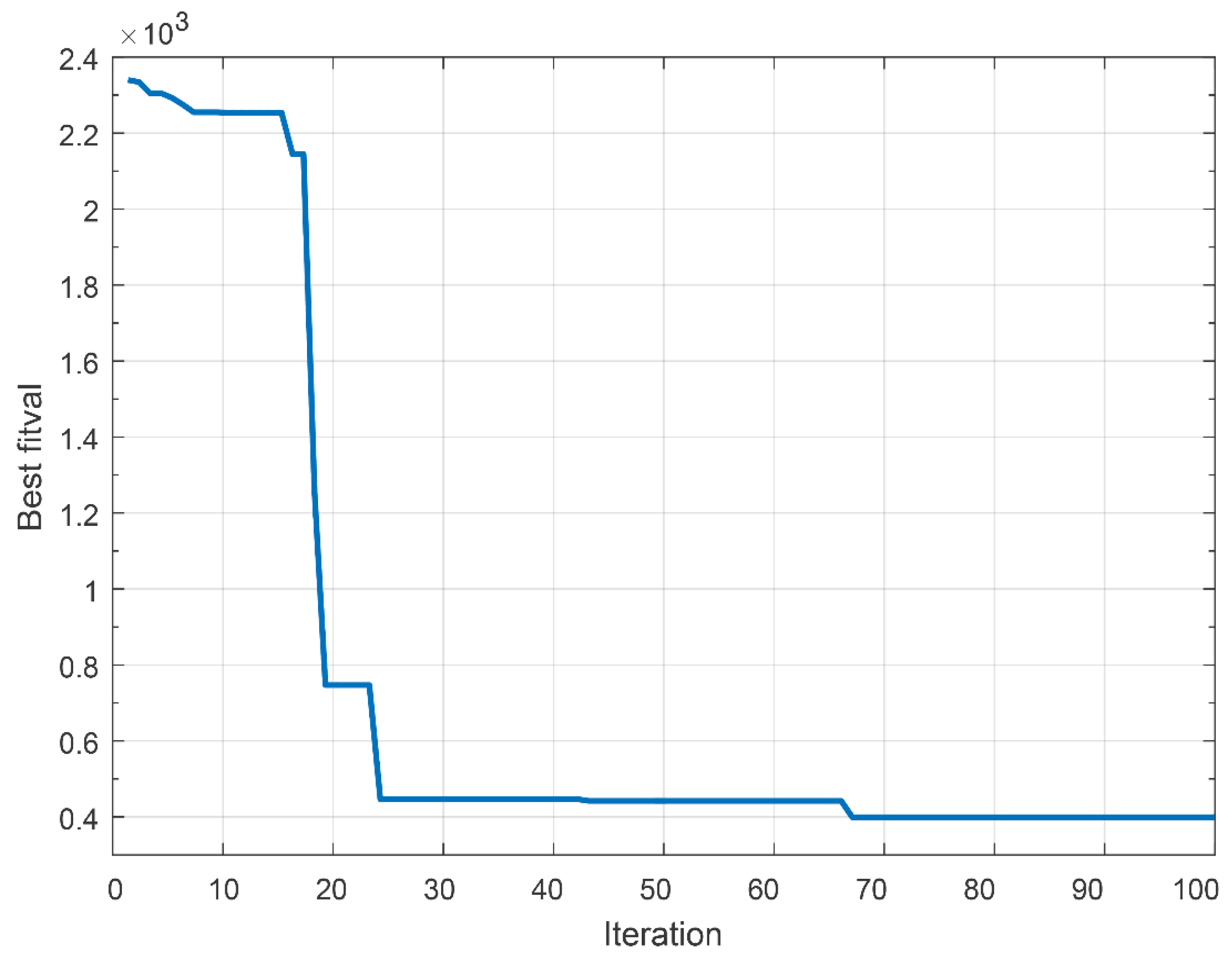
The proposed microgrid with initial scaling factors for inputs and output of FLC and basic membership functions were simulated within ABC optimization algorithm. The algorithm is run with different number iteration; 20, 50 and 100, for 86,400 s (24 h). The more iteration, the better optimization results. Figure 9 illustrates the optimization convergence during the simulation process for 100 iterations. Optimal scaling factors for FLC after optimization are exhibited in

Table 3. Optimal scaling factors for FLC obtained from ABC optimization algorithm.

Factor	Optimal Value
$K_{SOC}$	1.293
$K_{NetPower}$	0.706
$K_{FCPower}$	0.9012

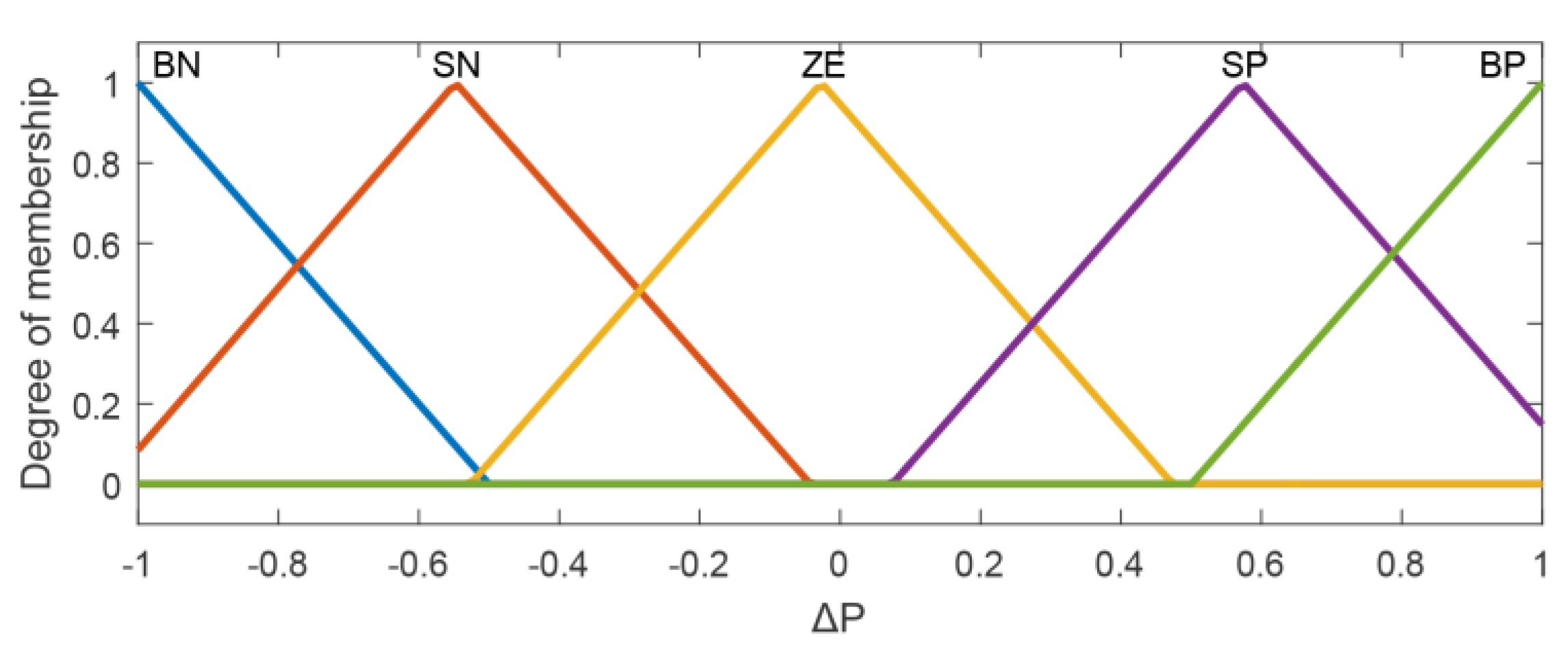
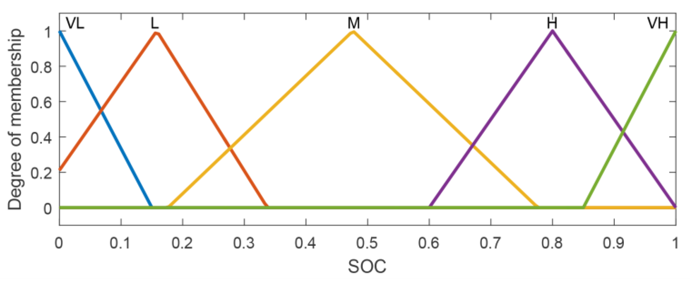
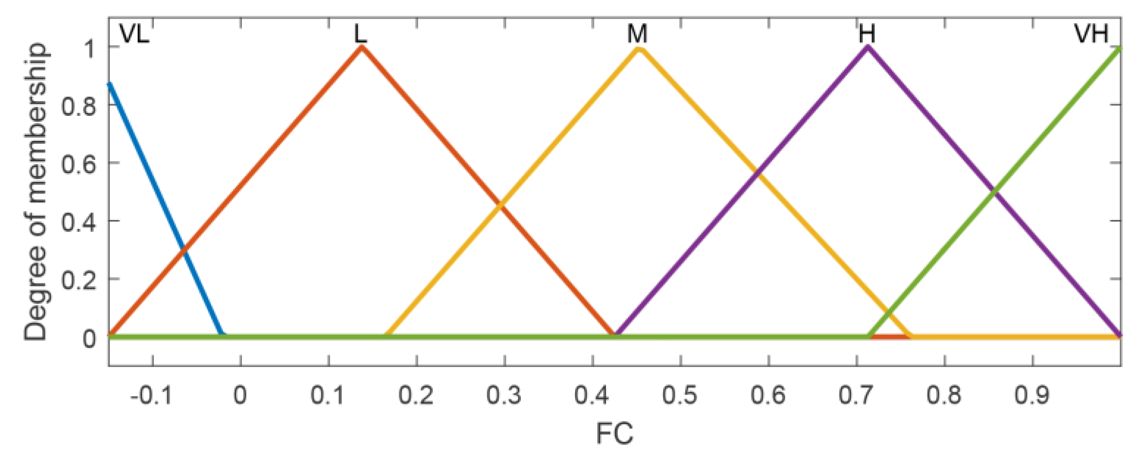
. Figure 10, Figure 11 and Figure 12 illustrate the optimized FLC membership functions.

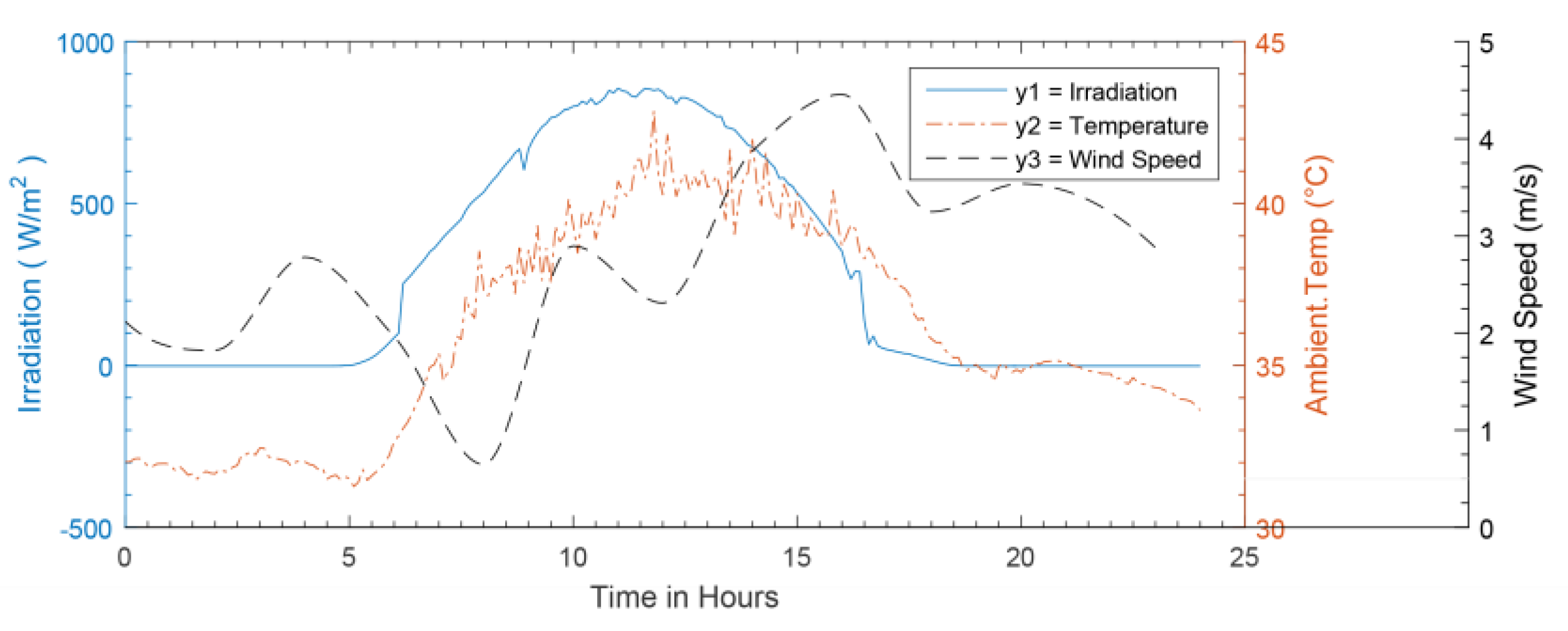
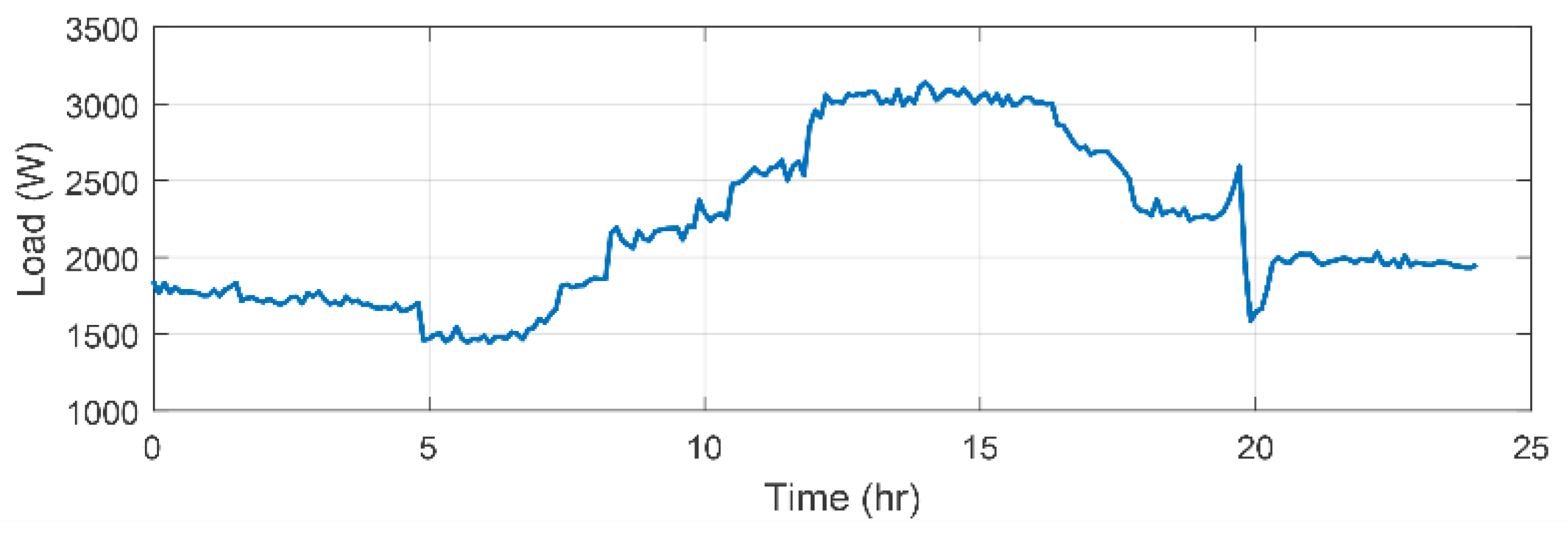
Figure 13 exhibits real data inputs that applied to the microgrid. It can be noticed from the house load profile shown in Figure 14 that midnight hours to early morning hours, the load demand is low. However, the PV generation still in its lower levels and low wind speed in Dhahran city at this period of the day which leads to low power generation from WT. Thus, the use of FC as a backup system is necessary to meet the load demand. The midday hours show high load consumption, however, the REG in its maximum levels also. Therefore, the load is successfully met by the REG and the surplus energy is charged to the BESS. The third period starts for sunset up to midnight. At the beginning of this period, the energy stored in BESS can supply the load demand and lasts for some hours. Then FC starts operation to meet the load demand according to the FLEMS control.

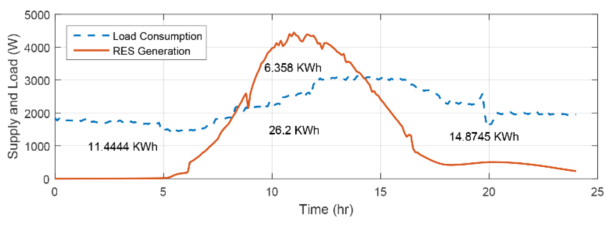
Figure 15 shows the energy analysis of the load demand compared with REG during the day hours. For the purpose of analysis, we calculate the Area Under the Curve (AUC) of the intersections between load demand and REG which gives us three main areas; the amount of energy that supplied by REG to the load demand, the amount of excess energy to be stored in BES, and the amount of energy to be compensated from the backup sources during the absence of REG. The amount of energy in the periods on left and right sides are not supplied by REG. Therefore, BES and FC should operate according to the FLEMS to meet this demand. On the top of Figure 15, the excess amount of energy from REG during midday hours that should be stored in the BES. 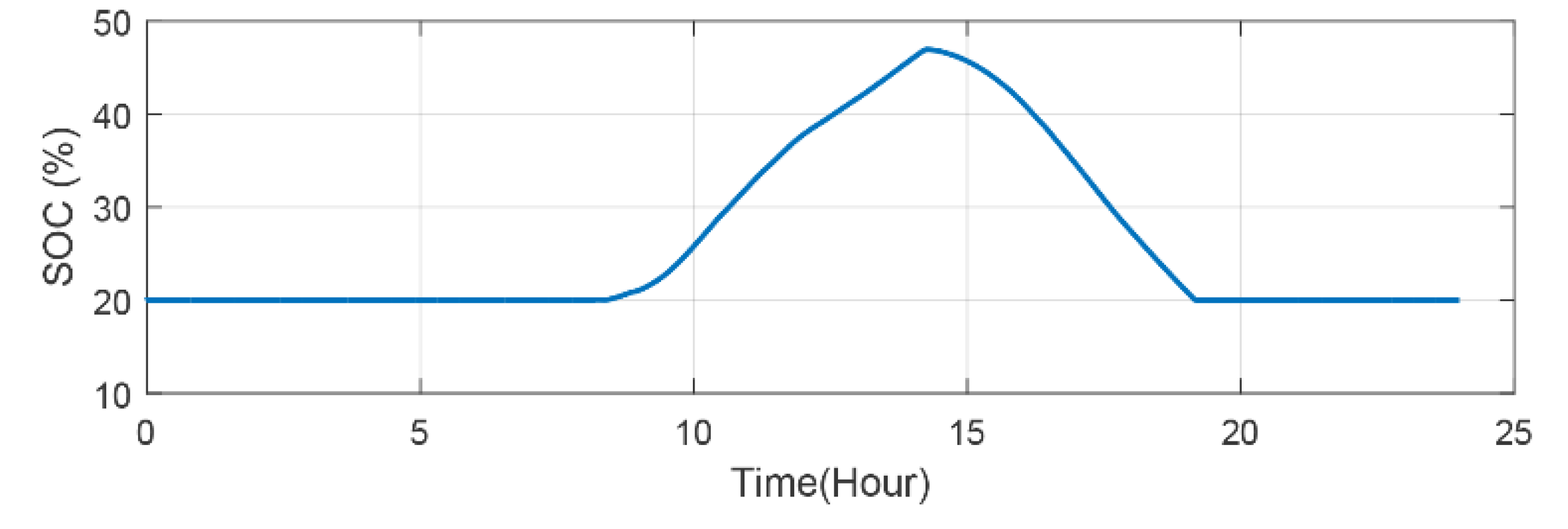Figure 16 presents the SOC of the BES during the day hours. Some losses in energy is existed and expected due to the power electronics devices. The energy analysis of BES during simulation of the day is presented in

Table 4. Battery energy storage (BES) energy analysis for 24 h.

Period	00:00 a.m−8:10 a.m	(Charging) 8:10 a.m–2:15 p.m	(Discharging) 2:15 p.m–5:00 p.m
Δ SOC	20%	20% to 47%	47% to 20%
Energy	0	5.4 kWh	5.4 kWh

. As mentioned in the methodology, the BSA gives the suitable size of the battery for all year seasons depending on the REG data for 365 days. In a typical summer day, as used in the simulation of this work, it is noticeable that the BES charged to nearly the half size of its capacity. This is due to the increased load demand during the summer season in the study location which means most of REG is used by the load during day hours and a small amount of energy stored in BES. Whereas in winter and autumn seasons, the load demand decreased by more than the half of that in the summer season, which means the excess REG during these seasons days needs enough BES size to be stored.

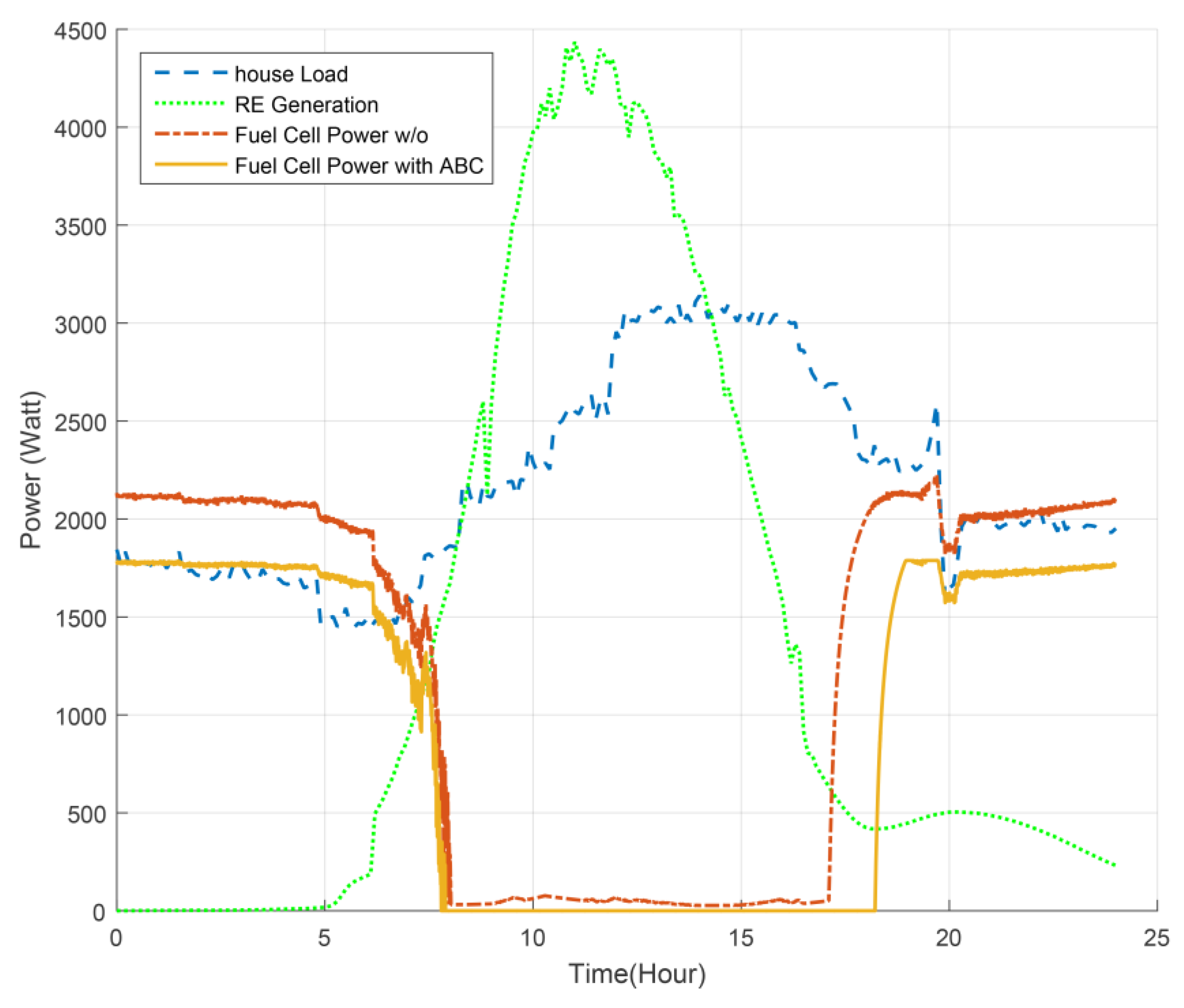
The operation of the FC during the day hours is shown in Figure 17 with/without the optimization of FLEMS using ABC algorithm. Before 8:00 a.m, it is noticeable that the operation of FC without optimization exceeds the total load demand need. This means that there is extra energy generated for no use due to the control of unoptimized FLEMS, hence, the total generation cost increased. On the other hand, the operation of FC controlled by optimized FLEMS is decreased and almost covered the load demand during the absence of REG and BES. In addition, after 8:00 p.m, the operation of FC using unoptimized FLEMS gives nearly the same load demand although the REG still generating power; most probably from WT due to moderate wind speed at that time (see Figure 13) this means there is an extra unused power generated from FC leads to increase in generation cost. However, the operation of FC controlled by optimized FLEMS generates almost the needed power for the load demand after the consumption of REG power, thus it appeared lower than load demand power in the graph. For the purpose of simplifying the simulation, the starting time of FC is neglected. Total energy analysis details of the proposed microgrid during the operation in the day hours are presented in

Table 5. Total microgrid energy analysis and system energy saving efficiencies on 28th of July 2016.

Parameter	Energy
Residential Load Consumption	52.5189 kWh
PV System Generation	28.7939 kWh
WT system Generation	3.7641 kWh
Total RE generation	32.558 kWh
Fuel Cell (with normal FLC)	29.3366 kWh
Fuel Cell (with optimized FLC)	22.4899 kWh
Without optimization	86.18%
With ABC optimization	97.07%

. Depending on the amount of energy that the microgrid should be supplied from backup systems during the day hours, system energy saving efficiency is calculated before and after optimization.

5.2. Optimized Microgrid FLEMS Considering Economic Dispatch

Simulation and results of the proposed method to enhance the performance of the optimized FLEMS depending on economic dispatch are presented in this section. Since diesel generator in this part replaces the wind turbine system, the economic dispatch problem is solved depending on real data for 24 h of the same summer day in the first stage using three different intelligent techniques which are: ABC, PSO and GA. Then, the microgrid is simulated using the best technique that minimizes the operation cost of the backup sources. Cost and efficiencies are calculated to prove the effectiveness of the proposed method.

Table 6. Generation cost of each optimization technique used in the Economic Dispatch (ED).

Optimization Technique	ABC	PSO	GA
ED Cost ($)	704.5295792	704.5253399	704.8097585

exhibits the generation cost of the dispatchable sources in the microgrid using the three optimization techniques.

When comparing the total cost for 24 h using different optimization techniques, it is obvious that ABC and PSO techniques reduce the cost more than GA. However, the PSO optimization technique is the best among the tree techniques with little difference when compared with ABC. Hence, PSO is used in the economic dispatch scheduling within FLEMS of the microgrid.

Table 7. Economic dispatch solution using the particle swarm optimization (PSO) Technique.

Time (h)	FC (W)	DG (W)	RE Gen. (W)	House Load (W)	BES (W)
1	1545.403	298.2779	0	1843.681	0
2	1467.416	283.1387	0	1750.555	0
3	1431.891	277.172	0	1709.063	0
4	1485.572	286.6482	0	1772.22	0
5	1403.547	270.7464	0	1674.293	0
6	1229.208	236.9774	0	1466.185	0
7	1211.029	233.2711	43.63771	1487.862	0
8	636.6834	122.2966	838.1992	1597.172	0
9	167.7575	31.5025	1662.303	1861.561	0
10	0	0	2572.191	2115.248	−456.94
11	0	0	3688.539	2286.499	−1402.02
12	0	0	4171.665	2553.053	−1618.612
13	0	0	4071.112	2959.199	−1111.913
14	0	0	3540.936	3095.96	−444.98
15	0	0	2660.951	3139.717	478.766
16	826.4287	159.0213	1650.371	3035.966	402.9997
17	908.5584	174.9316	720.9348	3002.192	1197.774
18	1152.026	222.0738	14.19419	2668.332	1280.088
19	2187.312	422.4882	0	2609.77	0
20	1911.005	368.995	0	2279.933	0
21	1388.388	267.8123	0	1656.186	0
22	1685.124	325.2758	0	2010.446	0
23	1667.578	321.8222	0	1989.327	0
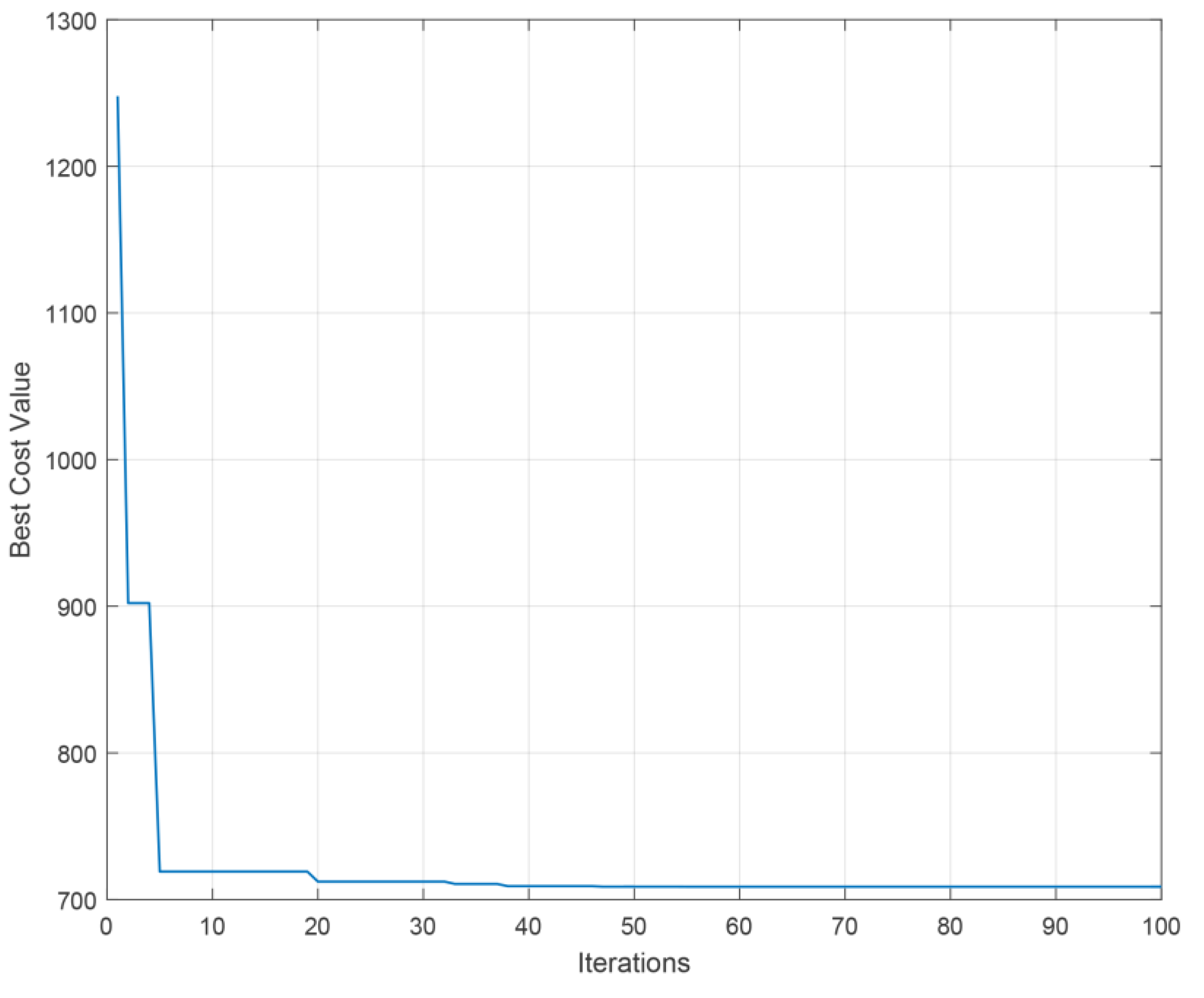
24	1639.153	316.3475	0	1955.419	0

exhibits the ED solution from PSO for 24 h of the microgrid on 28th of July 2016. Figure 18 illustrates the best cost value during the optimization process using PSO. It may be remarkable from the figure that the best cost value has been obtained at 20 iterations, however, PSO algorithm is still searching for optimal values of the dispatchable sources generation to reduce the cost up to 100 iterations. It is noticeable that there is a reduction at 32 and 40 iterations. There could be a slight reduction after that which is not seeable from the figure. The algorithm obtained the economic dispatch for the dispatchable sources for 24 h within a few seconds in simulation time because the load demand is already known before. However, in real time, the algorithm searching time will be decreased because the proposed system will solve the economic dispatch problem in an hourly manner. Table 7 presents the solution of the economic dispatch problem using the PSO algorithm at each hour of the day. The dispatchable sources are started to generate power from 12:00 a.m up to 9:00 a.m. At 9:00 a.m, the REG started (due to the increase of sun irradiation) to generate enough power to supply the load demand and the excess power is sent to the BES to be charged, so it appears to be minus in the last column of the table. This is the amount of power that to be stored in BES, however, there are some losses due to the power electronics in the microgrid system. At 3:00 p.m when the REG start to not generate enough power to the load demand (due to the decrease of sun irradiation), the BES starts to discharge to compensate the decrease in REG and continue to discharge up to 6:00 p.m. At that time, the FLEMS gives the dispatchable sources the whole responsibility to supply the load demand according to the economic dispatch limits. 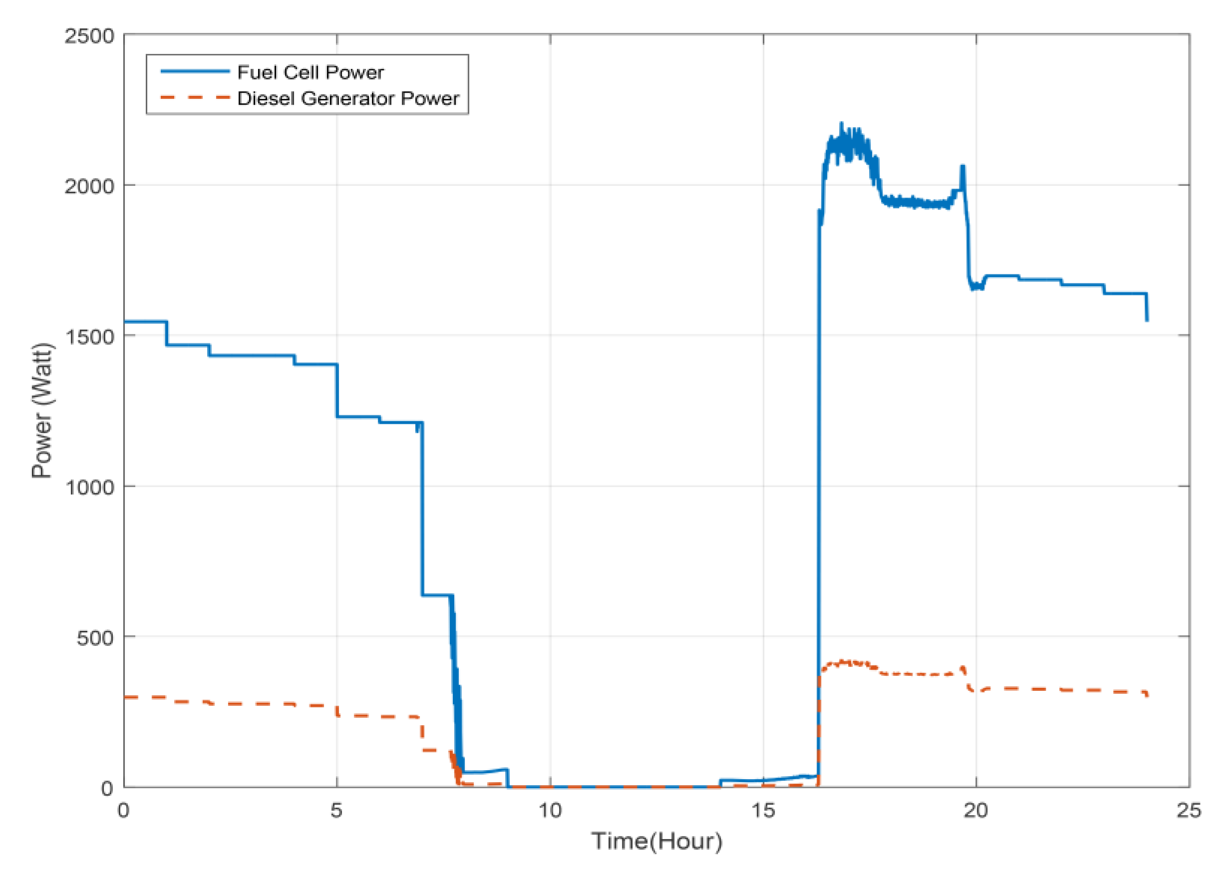Figure 19 shows the operation of the dispatchable sources of the microgrid on the same day.

To investigate the effectiveness of the proposed method using economic dispatch within the microgrid FLEMS, three different scenarios are simulated:

• Microgrid that has PV and WT as RES operating with FC and BES as a backup system controlled by FLEMS without optimization.
• Microgrid that has PV and WT as RES operating with FC and BES as a backup system controlled by optimized FLEMS using ABC.
• Microgrid that has only PV as RES operating with FC, DG and BES as a backup system controlled by optimized FLEMS considering economic dispatch.

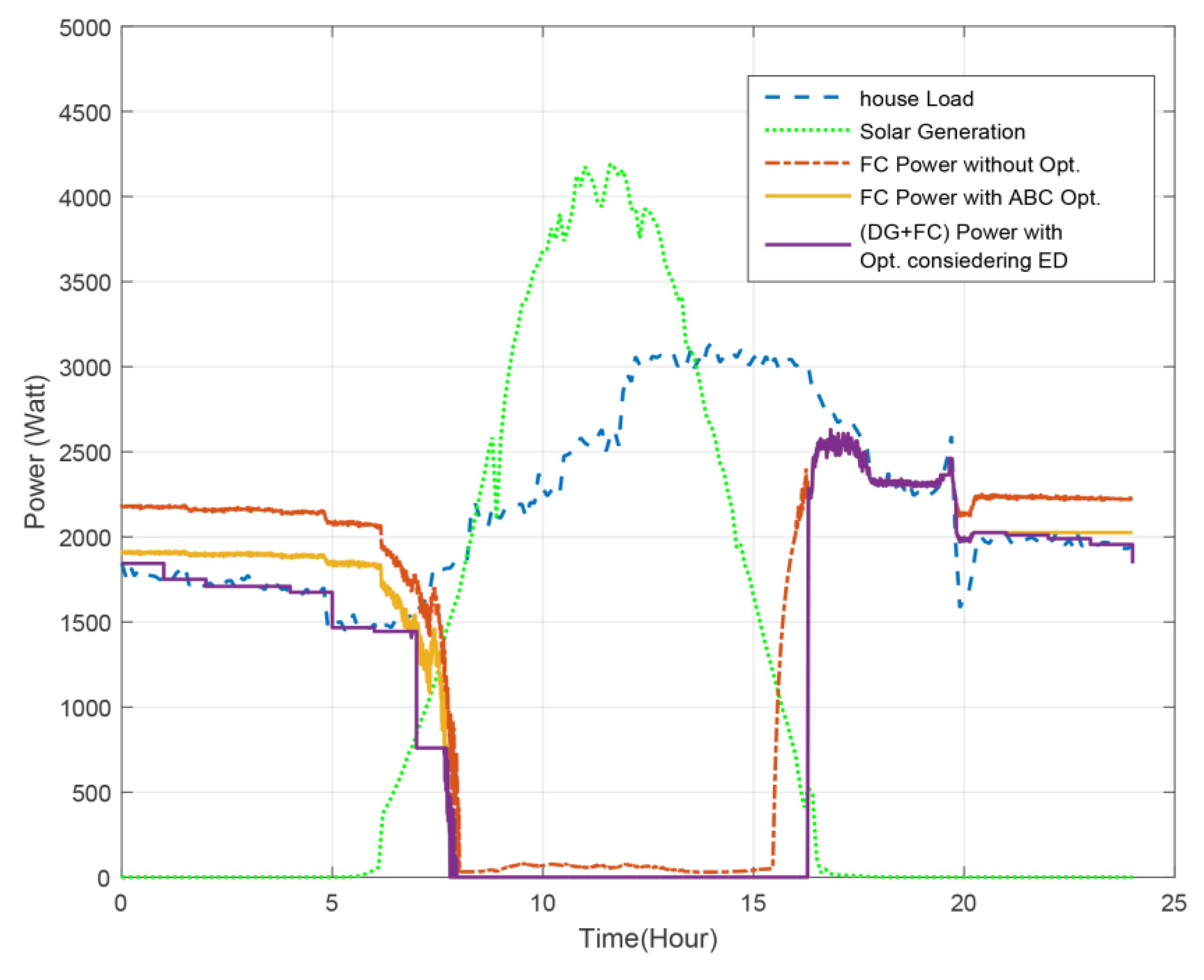
A comprehensive view of the microgrid operation for 24 h with three different scenarios is illustrated in Figure 20. It is noticeable that the use of FLEMS considering economic dispatch decrease the generation of dispatchable sources to the level of the load demand, hence the system efficiency increased in terms of energy saving and the generation cost decreased as presented in

Table 8. System efficiency in three different methods.

Method	Efficiency
MG controlled by FLC without optimization	86.97%
MG controlled by FLC with ABC optimization	94.5%
MG controlled by FLC with ABC optimization considering ED	97.67%

and

Table 9. Cost comparison between optimized FLC using ED and conventional ED operation.

Method	Cost/day
operation using ED only	704.53
operation by opt. FLC considering ED	625.65

.

Table 8 exhibits the efficiency of the system in the three scenarios. The results show that the proposed method has the most efficient operation for 24 h of the day.

A cost calculation is done to compare the proposed method in this work with conventional economic dispatch scheduling. The exhibited results in Table 9 show that the proposed method reduces the cost by 11.19%.

6. Conclusions

An optimized fuzzy logic energy management system has been proposed for a standalone DC microgrid consisting of solar photovoltaic panels, wind turbine, battery energy storage, fuel cell and diesel generator supplying a typical residential load. The system is controlled by a low complexity fuzzy system with only 25 base rules. The overall system is mathematically modeled and the optimization problem is solved using an artificial bee colony, which gives better results in terms of control and energy saving efficiency that has been improved by 10.89%. Furthermore, the proposed microgrid fuzzy based energy management system is considered as an economic dispatch problem, and the simulation results show enhancement in control, energy saving by 10.79% from unoptimized FLEMS and by 3.17% from the optimized FLEMS in the first stage, and reduction in generation cost when compared with conventional economic dispatch methods by 11.19%. All simulations were performed in MATLAB/Simulink environment using long-term real data of solar irradiation, ambient temperature, and wind speed of 2016 calendar year from Dhahran City located in the eastern region in Saudi Arabia. The methodology can, however, be easily extended to other regions and datasets.