Assessment of Maximum Penetration Capacity of Photovoltaic Generator Considering Frequency Stability in Practical Stand-Alone Microgrid

Abstract

In South Korea, the existing diesel generators are being replaced with renewable energy sources (RESs) in several stand-alone microgrids. However, their reliability and stability are not still guaranteed by fluctuations of the system caused by RESs, arising from unpredictable changes in environmental factors. Moreover, since the inertia that is originally provided by the diesel synchronous generators is reduced, the overall system becomes highly sensitive to frequency variations. As a result, the installation of RESs must be well planned while considering the upper limit of their installed capacity. In this paper, a new method for evaluating the maximum penetration capacity of photovoltaic (PV) generators to ensure the stable operation of a microgrid is proposed. For the analytical approach, two frequency stability indexes, which are the minimum instantaneous frequency and the quasi-steady-state (QSS) frequency after a disturbance, are used. The capacity of PV to be installed is limited by considering the characteristics of other generators. In addition, the efficiency of the energy storage system (ESS) is also analyzed to determine the optimal capacity of both PV and ESS. The effectiveness of the proposed method is firstly proven through the mathematical analysis. Then, case studies on a practical stand-alone microgrid in South Korea are carried out using a time-domain simulation based on the DIgSILENT PowerFactory^® software.

1. Introduction

Most recently, stand-alone microgrids are involved in a great transition with the high penetration of renewable energy sources (RESs) by replacing conventional diesel synchronous generators. In other words, for microgrids, which were previously operated with only diesel generators, the entire topology of system is being changed in the form of distributed energy resources (DERs) [1,2]. In this case, the entire planning process must be redesigned to ensure stable operation of the microgrid. However, the high penetration of RESs, which are mainly wind turbine (WT) and photovoltaic (PV) generators, may increase the uncertainty in the power system while causing large frequency variations. Therefore, stand-alone microgrids, which are isolated from the main grid, must include dispatchable generators in order to overcome the uncertainty from RESs.

The size and placement of RESs can be optimized using electrical system data (e.g., frequency limits, voltage limits, system protection equipment, settings, etc.) and RES data (e.g., type of generator, operation modes, potential locations, etc.) [3]. Furthermore, the system design, which can ensure frequency stability, is necessary because the frequency relay in the microgrid operates when the system frequency varies beyond its limits while causing unwanted blackout. Thus, the frequency stability must be considered to calculate the maximum penetration capacity of RESs for a stand-alone microgrid with high renewable penetration.

Several studies [4,5,6,7,8,9,10,11] were carried out for the stability of system frequency when the level of renewable penetration was increased. In Reference [4], the system frequency response was analyzed for different wind power penetration levels, and an optimal parameter range for a controller was derived. Also, the method to increase the penetration level of RESs by using the storage characteristics of an energy storage system (ESS) was described in Reference [5]. In Reference [6], inertial control for a WT was proposed to stabilize the stand-alone microgrid. In addition, the control method of ESS was proposed to accommodate wind power fluctuations in [7]. The genetic algorithm (GA)-based method was proposed in Reference [8] for an optimal charging/discharging scheduling of ESSs, which are interconnected with PV. Furthermore, the integrated wind, solar, and energy storage plant, which mitigates power generation with a complementary generation profile, was introduced in Reference [9]. Hence, to increase the renewable penetration level of the grid, various frequency control methods were studied. In Reference [10], the ESS provided inertial and primary reserves to enhance the frequency stability, and it was sized in terms of required power and energy. Also, the supplementary droop control method was introduced to improve the stability of the microgrid in Reference [11]. However, it is essential to precisely determine the maximum penetration capacity of PV because the PV generators lack adaptive control technologies, such as inertial control in WTs.

Few studies were reported on the capacity calculation of the RESs. Instead, most papers focused on the optimum sizing of ESS. In Reference [12], the methodology for planning the energy and power capacity of ESS was proposed in order to smooth the fluctuation from RESs. The ESS sizing method to increase the renewable penetration in terms of grid frequency deviations was introduced in Reference [13]. In Reference [14], the probabilistic approach for the optimal capacity specification of renewable integrated ESS was tested using real wind data. The assessment of maximum capacity for DERs was given in Reference [15]. However, multiple operation scenarios must be analyzed by using a probabilistic method, which is time consuming.

In this paper, an algorithm to evaluate the maximum penetration capacity of PV is proposed. It determines the capacity of the PV based on both maximum quasi-steady-state (QSS) and instantaneous frequency deviation limits, which are given by the system operator reflecting the characteristics of the microgrid. Then, the magnitude of a credible contingency event is derived by using the dynamic droop equation while considering the droop coefficient and reserve powers at the initial and post-contingency state of diesel generators. Thereafter, the maximum penetration capacity of PV is evaluated from the perspective of QSS frequency. Finally, a time-domain simulation is carried out to determine whether the frequency stability of the microgrid is ensured based on the required limits of the QSS and instantaneous frequency. In conclusion, the main contributions of this paper are summarized as follows:

• The maximum penetration capacity of PV is evaluated to satisfy the frequency stability of a stand-alone microgrid;
• A new dynamic droop equation is derived by considering both the droop coefficient and reserve power of each generator instead of the droop coefficient for entire system;
• Case studies are carried out by using the practical data of stand-alone microgrid in South Korea.

This paper is organized as follows: firstly, a theoretical background for four stages of the frequency responses for a stand-alone microgrid is described in Section 2. Then, the method to evaluate the maximum penetration capacity of PV is proposed in Section 3. A model of a practical stand-alone microgrid with diesel generators, PV generators, and ESSs is described in Section 4. Next, several case studies are carried out on the stand-alone microgrid with high renewable penetration by using both analytic analysis and time-domain simulations based on DIgSILENT PowerFactory^® software in Section 5. Finally, conclusions are given in Section 6.

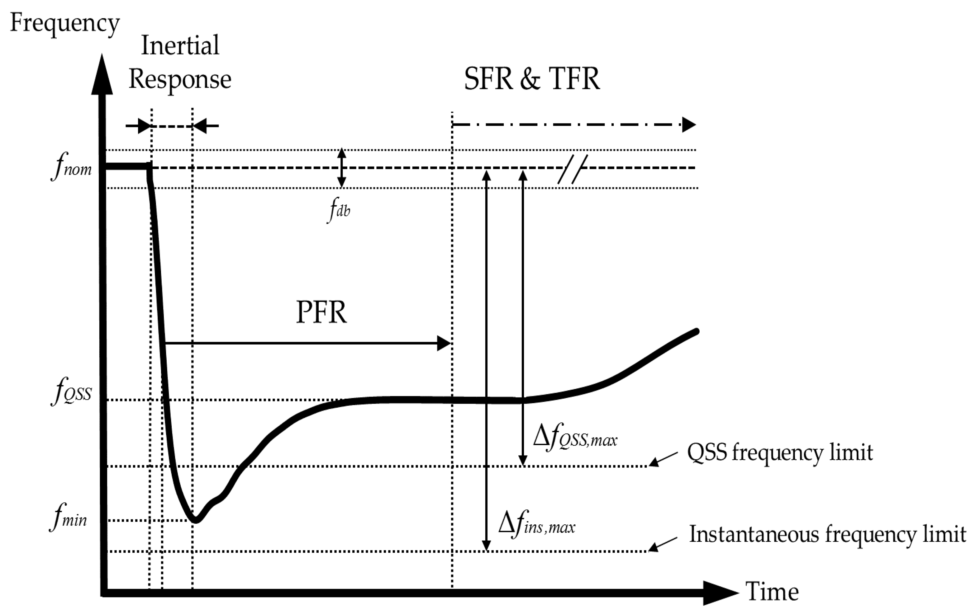
2. Frequency Response of Microgrid with High Renewable Penetration

Most power systems have hierarchical controls to eliminate power imbalances rapidly and reliably after a disturbance, by which the system frequency is reduced from its nominal value, f_nom, by more than a deadband, f_db. They can be divided into three levels, which are the primary, secondary, and tertiary controls. However, the frequency response behavior can be classified into four stages, as shown in Figure 1 [16]. The first stage is the inertial response, which is uncontrolled because the power imbalance is instantaneously and naturally resolved by the stored kinetic energy of synchronous generators. In other words, the power output will be increased for a short time as the rotational energy in the synchronous generator is released to mitigate the fluctuation in system frequency. The second stage is the primary frequency response (PFR), in which the power imbalance is eliminated by the power output control of each generator, depending on the frequency deviation. With this control, also referred to as droop control, the system frequency is settled to the QSS value, f_QSS, where a power balance is ensured. Then, the secondary frequency response (SFR) follows to compensate for the system frequency deviation from its nominal value (i.e., 60 Hz). Finally, the tertiary frequency response (TFR) relates to long-term operations making the generators operate at their optimal point.

In the stand-alone microgrid, the system frequency lasts at f_QSS for a long duration since the secondary control acts more slowly than in larger power systems. Furthermore, the minimum instantaneous frequency, f_min, occurs during the PFR stage as shown in Figure 1. Both the deviation of QSS and instantaneous frequency should not exceed their limits (Δf_QSS,max and Δf_ins,max, respectively) to ensure the frequency stability of the stand-alone microgrid. Therefore, the maximum penetration capacity of PV must be evaluated in terms of f_QSS and f_min, which are described in the subsequent sections.

2.1. Quasi-Steady-State Frequency

The droop control is generally used as the primary control in a microgrid [17]. When a number n of generators in a power system utilize the droop control, the deviation of system frequency for the QSS, Δf_QSS, can be calculated for the entire system according to the droop equation as follows:

$$\Delta f_{QSS}=f_{nom}-f_{QSS}=-R_{sys}\times \Delta P,$$

(1)

$$R_{sys}=\frac{{\displaystyle {\sum }_{i=1}^n{R}_i\times P_{i,\mathit{max}}}}{{\displaystyle {\sum }_{i=1}^n{P}_{i,\mathit{max}}}},$$

(2)

where the R_sys is the droop coefficient of the entire power system, and the ΔP is the deviation of active power generation caused by a disturbance. The R_i and P_i,max are the droop coefficient and maximum power output limit of the i-th generator, respectively. However, when the renewable penetration level of system is high, the reserve power of each generator may be insufficient even if the reserve power of all generator is enough. If the power output of diesel generator reaches its limit before the system frequency settles, both R_sys and f_QSS will decrease. Therefore, Δf_QSS must be calculated by considering the reserve power of each diesel generator.

2.2. Instantaneous Frequency

When the system frequency is significantly reduced, load shedding may be induced to prevent the outage in the generator from rotating beyond the operating speed range. Therefore, the instantaneous frequency must be maintained higher than the outage point. Both the system droop coefficient and inertia constant of the system are important factors for computing f_min, which is observed in the PFR stage. The system inertia constant, H_sys, is calculated as follows:

$$H_{sys}=\frac{{\displaystyle {\sum }_{i=1}^n{H}_i\times S_i}}{{\displaystyle {\sum }_{i=1}^n{S}_i}},$$

(3)

where the H_i and S_i are the inertia constant and apparent power of the i-th generator, respectively. However, because the exact value of f_min is difficult to calculate, the swing equation is used to indirectly assess the value. The effect of the inertia on the system frequency is given as follows:

$$\frac{df}{dt}=\frac{f_{nom}}{2H_{sys}}\times \left(P_m-P_e\right),$$

(4)

where the df/dt is the rate of change of frequency (RoCoF), and P_m and P_e are the mechanical power and electrical power, respectively. From Equation (4), it is obvious that the grid with a larger inertia constant will have the higher f_min. However, the RoCoF is also affected by the response time of how closely P_m follows the reference signal, P_e. Therefore, the response time of a generator is difficult to obtain numerically. Instead, it can be estimated from time-domain simulations.

3. Evaluating Maximum Penetration Capacity of PV

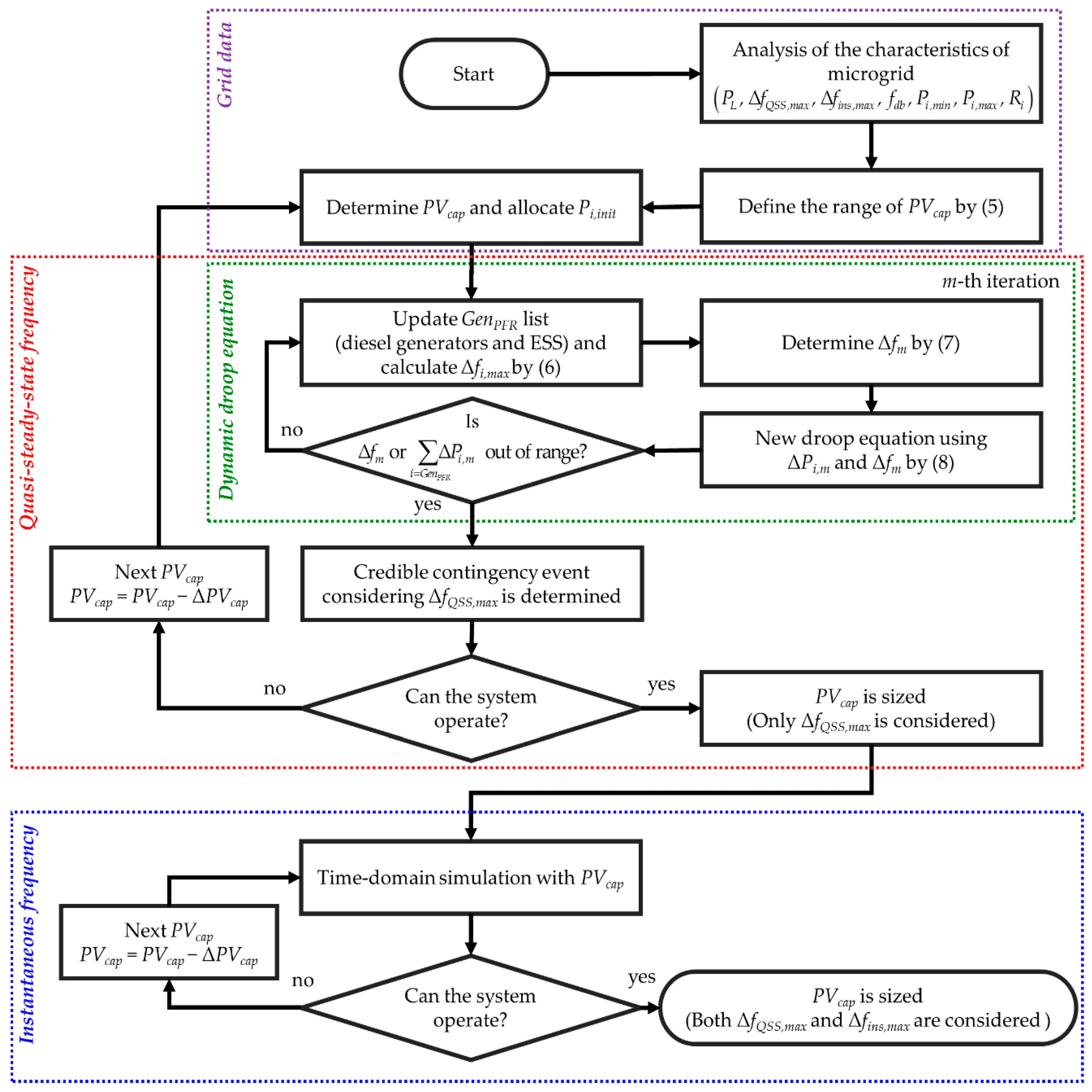
3.1. Methodology

Figure 2 shows the proposed algorithm for evaluating the maximum penetration capacity of PV. The algorithm is divided into four parts. Firstly, the characteristics of system are analyzed. Then, the new dynamic droop equation is generated by considering the power output limits of each generator. Thereafter, the penetration capacity of PV is evaluated based on the QSS frequency. Finally, the size of PV is determined based on the instantaneous frequency by using time-domain simulations.

3.1.1. Analysis of Characteristics of Microgrid

Firstly, the desired numbers of operating diesel generators and ESSs are set, as well as the load demand. Then, the required frequency limits, the maximum QSS (Δf_QSS,max) and instantaneous (Δf_ins,max) frequency deviation limits, and frequency deadband (f_db) are specified. In addition, data for the minimum (P_i,min) and maximum (P_i,max) power output and the droop coefficient (R_i) of i-th generator are required. Once the number of operating diesel generators and the load demand, P_L, are determined, the capacity range of PV can be specified as follows:

$$P_L-\underset{i=diesel}{{\displaystyle \sum P_{i,\mathit{max}}}}<P{V}_{cap}\le P_L-\underset{i=diesel}{{\displaystyle \sum P_{i,\mathit{min}}}},$$

(5)

where the PV_cap is the capacity of PV. For the first loop in the proposed algorithm, PV_cap is set to the maximum value within its range. With each iteration, it is reduced by the value of ΔPV_cap. Then, the initial power outputs of the i-th generator, P_i,init, are allocated to each generator.

3.1.2. Droop Equation Considering the Power Output Limit

Next, the new dynamic droop equation is derived for the target microgrid. The equation is derived to calculate the relationship between the frequency deviation and power deviation by using not only the system droop coefficient in Equation (2), but also the power output limits and reserve power of each generator. The generators and ESSs with sufficient reserve power to participate in PFR control are classified as GenPFR. Then, the maximum variable frequency deviation Δf_i,max for the i-th generator in the Gen_PFR list is calculated as follows:

$$\Delta f_{i,\mathit{max}}=-R_i\times \left(P_{i,\mathit{max}}-P_{i,init}\right).$$

(6)

Afterward, the deviation of system frequency in the m-th iteration, Δf_m, is determined by comparing with the required limit of Δf_QSS,max as follows:

$$\{\begin{array}{cc}\Delta f_m=\Delta f_{QSS,\mathit{max}}-f_{db},& if\mathit{min}\left(\Delta f_{i,\mathit{max}}\right)\ge \left(\Delta f_{QSS,\mathit{max}}-f_{db}\right)\\ \Delta f_m=\mathit{min}\left(\Delta f_{i,\mathit{max}}\right),& if\mathit{min}\left(\Delta f_{i,\mathit{max}}\right)<\left(\Delta f_{QSS,\mathit{max}}-f_{db}\right)\end{array}.$$

(7)

The frequency can fluctuate up to the limit of (Δf_QSS,max − f_db). However, when the frequency deviation reaches to the minimum among the values of Δf_i,max (i.e., min(Δf_i,max)), the generators without sufficient reserve power are unable to participate in PFR control. Therefore, the droop coefficient of the entire system must be updated in real time with the GenPFR list. As a result, the droop equation, which calculates the deviation of the system frequency, is derived as follows:

$$\Delta f=-\frac{\underset{i=GenPFR}{{\displaystyle \sum R_i\times P_{i,\mathit{max}}}}}{\underset{i=GenPFR}{{\displaystyle \sum P_{i,\mathit{max}}}}}\left(P-\underset{i=GenPFR}{{\displaystyle \sum \Delta P_{i,m}}}\right)+\Delta f_m+f_{db},\mathrm{for}\underset{i=GenPFR}{{\displaystyle \sum \Delta P_{i,m}^{old}}}<P\le \underset{i=GenPFR}{{\displaystyle \sum \Delta P_{i,m}}},$$

(8)

where ΔP_i,m is the deviation in active power when the system frequency varies by Δf_m, and $\Delta P_{i,m}^{old}$ is the deviation in active power from the previous iteration. The value of $\Delta P_{i,m}^{old}$ is zero in the first iteration. Next, the loop continues until the deviation of either the system frequency or the active power varies beyond their range, which can be determined as follows:

$$\Delta f_m<\left(\Delta f_{QSS,\mathit{max}}-f_{db}\right);$$

(9)

$$\underset{i=GenPFR}{{\displaystyle \sum P_{i,\mathit{min}}}}\le \underset{i=GenPFR}{{\displaystyle \sum P_{i,m}}}<\underset{i=GenPFR}{{\displaystyle \sum P_{i,\mathit{max}}}}.$$

(10)

Note that all loads are assumed to be a constant power model. Thus, variations in load demand due to changes in system frequency or bus voltage are ignored.

3.1.3. Quasi-Steady-State Frequency Viewpoint

After the droop equation is derived, the magnitude of credible contingency can be derived from the maximum value of P in Equation (8). If the size of contingency is smaller than PV_cap, the microgrid cannot operate. This loop is repeated by reducing the PV_cap until the microgrid becomes operable. Finally, PV_cap is determined based on the QSS frequency. Figure 3 shows the droop curves obtained from Equation (8) with seven (three 375-kVA and four 625-kVA) diesel generators participating in the power generation of microgrid. By using the proposed algorithm, the frequency deviation with uneven allocation of diesel generators can be calculated as shown by the black solid line in Figure 3. In this case, the power from one 625-kVA and one 375-kVA diesel generator reaches to the maximum output limits; thus, they are eliminated in the GenPFR list before the system frequency reaches to 59 Hz. The results show that the magnitude of credible contingency is 839.9 kW. However, the red dashed line shows that an even allocation of power generation based on the capacity of the generators allows the maximum contingency of 918.3 kW. Thus, the system without the ESS can operate the PV generator of 918.3 kW, which is approximately 31.67% of the total capacity of diesel generators. Note that the red dashed line is straight, but the black line is bent in the middle. The droop curve for the microgrid including a 400-kW ESS with the droop coefficient of 1% is shown by the blue dash-dotted line. The ESS is eliminated in the GenPFR list at 59.35 Hz as highlighted with the blue circle; thus, the droop coefficient of the entire system will decrease at that point. Because all of the reserve power of ESS is used for PFR before the frequency of 59 Hz is reached, the microgrid with ESS can operate the PV with the same capacity as that of ESS. Thus, the microgrid with the ESS of 400 kW can handle a contingency event of up to 1318.3 kW.

3.1.4. Instantaneous Frequency Viewpoint

Finally, PV_cap is determined in terms of the minimum instantaneous frequency by the results from time-domain simulations. In other words, the corresponding case simulation is carried out, and PV_cap is reduced by the value of ΔPV_cap until f_min reaches Δf_ins,max.

4. System Model of Microgrid

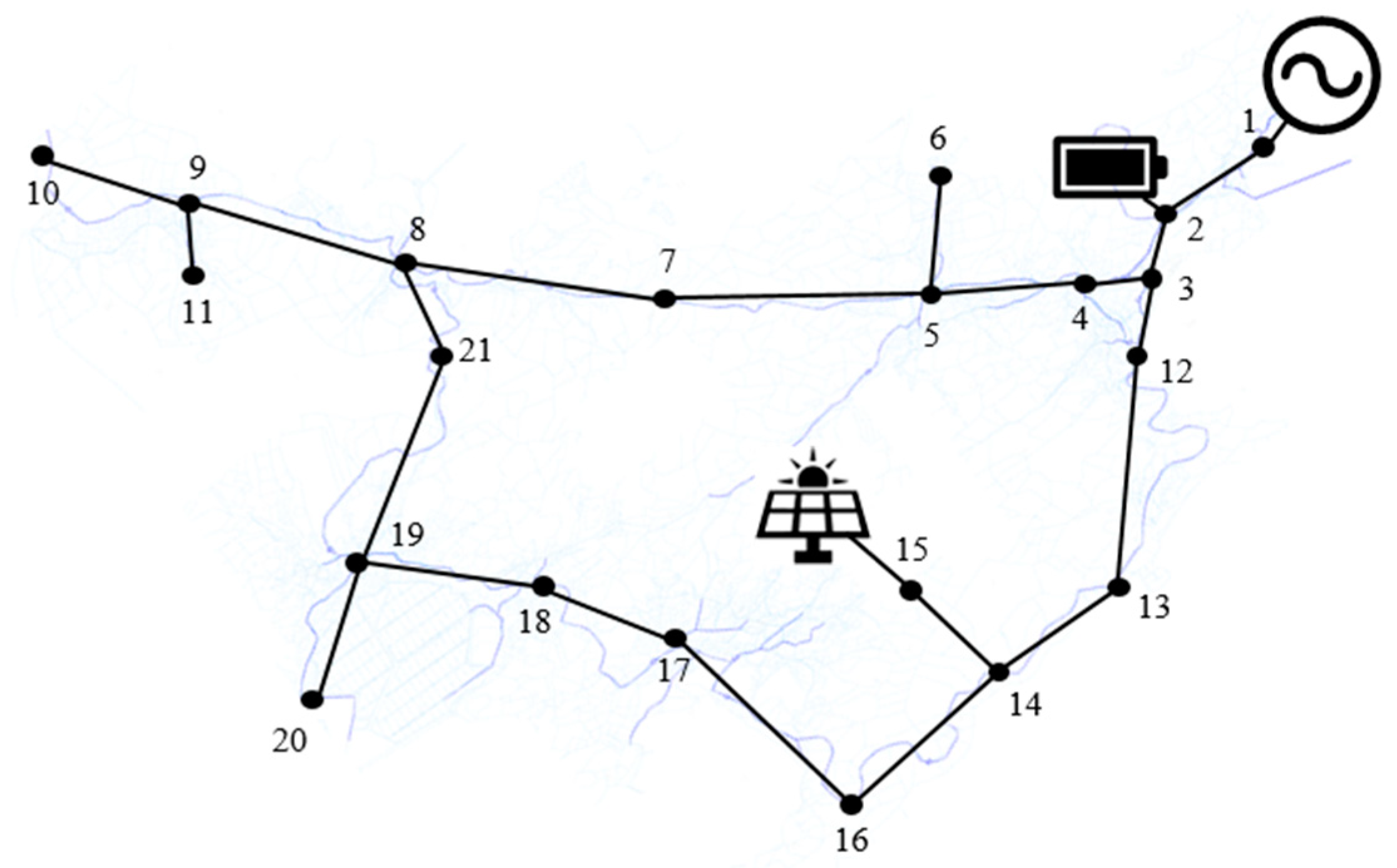
4.1. Practical Microgrid System in South Korea

The practical stand-alone microgrid system of “D” island in South Korea was considered to evaluate the maximum penetration capacity of PV, as shown in Figure 4. In this microgrid, diesel generators produce most of the power. However, a large amount of PV and ESS units were installed for their replacement. The locations of loads, diesel generators, PV, and ESS units were determined by the Korea Electric Power Corporation (KEPCO) in South Korea. The parameters and load demands utilized in this paper for the microgrid system are shown in

Table 1. Parameters of “D” island.

System Parameters
Diesel generators	375-kVA × 3, 625-kVA × 4
Line impedance	0.8991 + j0.4558 Ω/km
Nominal voltage	6.9 kV
Nominal frequency	60 Hz
Total load demands	1600 kW

and

Table 2. Load demands of “D” island.

Bus No.	Load		Bus No.	Load		Bus No.	Load
	P (kW)	Q (kVAR)		P (kW)	Q (kVAR)		P (kW)	Q (kVAR)
1	0	0	8	8.65	0.87	15	0	0
2	0	0	9	141.24	14.12	16	37.47	3.75
3	111.83	11.183	10	291.12	29.11	17	144.12	14.41
4	145.56	14.56	11	193.12	19.31	18	75.81	7.58
5	41.16	4.12	12	136.91	13.69	19	11.53	1.15
6	7.84	0.78	13	25.94	2.59	20	25.94	2.59
7	34.59	3.46	14	37.47	3.75	21	129.70	12.97

. In addition, each diesel generator used in this microgrid is described in the upcoming sections.

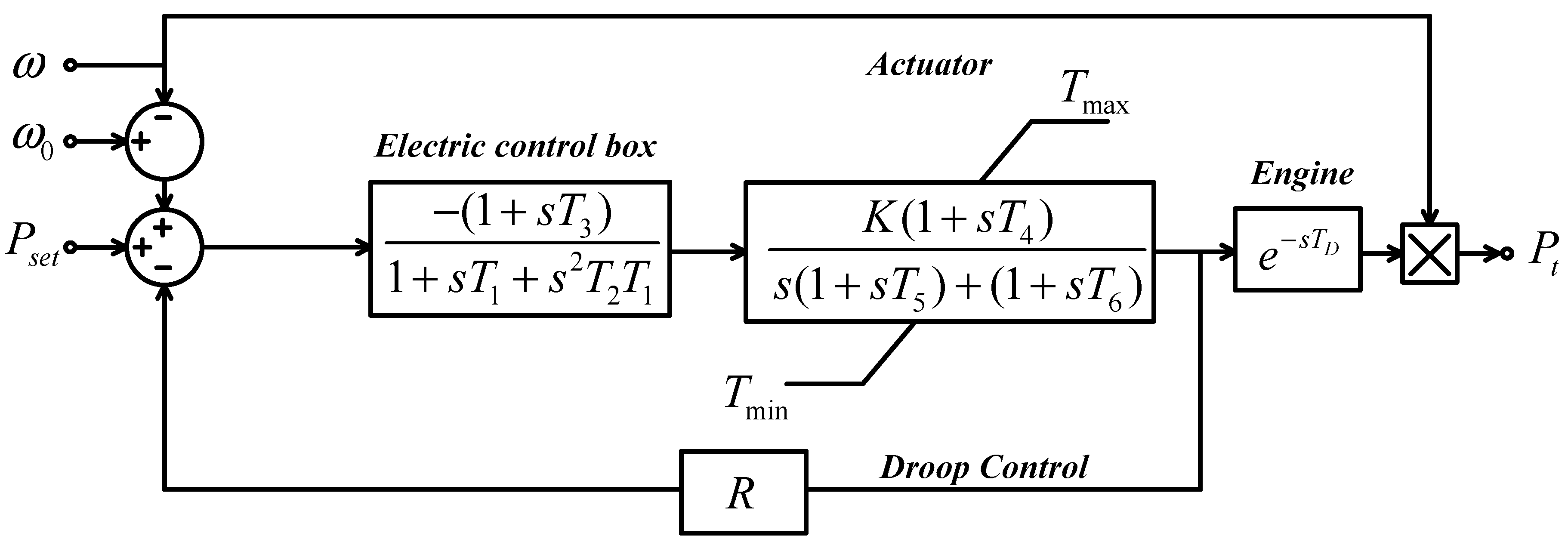
4.1.1. Diesel Generator

The practical microgrid has a total of seven diesel generators. Three are 375-kVA generators, and the other four are 625-kVA generators. The detailed parameters of each diesel generator are given in

Table 3. Parameters of the diesel generators in “D” island.

Parameters	375-kVA Model	625-kVA Model
Nominal voltage	6.6 kV	6.6 kV
Power factor	0.8	0.8
Inertia constant H	6.0 s	1.3007 s
Maximum active power Pmax	300 kW	500 kW
Minimum active power Pmin	120 kW	200 kW

. Due to their maximum and minimum power limits, the numbers of operable generators are determined according to the load demand. Figure 5 and

Table 4. Coefficients of the DEGOV1 model [18].

K	T1	T2	T3	T4	T5	T6	Te	Td	R	Tmin	Tmax
15	0.2	0.1	0.5	1	0.1	0.2	0.1	0.01	0.05	0	1.1

show the DEGOV1 governor model for the diesel generator and its coefficients used in this paper [18], respectively. The droop coefficients of all diesel generators were set to 5%, which is the typical value for “D” island.

4.1.2. Photovoltaic Generator

In evaluating the maximum penetration capacity of PV, the worst case for a practical microgrid was selected and analyzed to determine whether the grid can withstand those events. Accordingly, the PV generator had the following features:

• The PV used the maximum power point tracking (MPPT) control method to maximize its efficiency and power generation.
• For the microgrid with a high penetration level of PV generator, the worst contingency event will be a sudden change in solar irradiation, which causes the power output from the PV generator to reduce to zero. Such an event might occur frequently because the PV generators in this microgrid are concentrated within a small area.

4.1.3. Energy Storage System

The ESS was controlled by the droop method like the diesel generators. Thus, the ESS had the following characteristics:

• The ESS supplied the active power to the grid when the required power generation decreased below the load demand. In contrast, the ESS was charged when the power generation exceeded the load demand or when the state of charge (SOC) was substantially insufficient. Therefore, the ESS was in a standby state with the output of zero under normal conditions.
• The ESS increased the reserve power of system, which was used for the credible contingency event with a greater magnitude.
• The droop coefficient of ESS was set to be lower than that of the diesel generators. That is, the value was set to 1%.

5. Simulations and Results

To verify the effectiveness of the proposed evaluation method, several case studies were carried out on the practical stand-alone microgrid modeled in Section 4. Firstly, the capacity range of PV was determined based on the number of operating diesel generators. Then, the mathematical analysis was performed by using the dynamic droop equations to compute the magnitude of the maximum credible contingency event, as shown in

Table 5. Mathematical analysis results for quasi-steady-state frequency without the energy storage system (ESS).

Numbers of Operating Diesel Generators		PVcap Range (kW)	Credible Contingency Event (kW)	Maximum PVcap (kW)	Case Study
375-kVA	625-kVA
3	4	PVcap ≤ 440	918.3	440
3	3	PVcap ≤ 640	760	640
3	2	PVcap ≤ 840	601.6	601	1D
3	1	200 < PVcap ≤ 1040	433.3	433
3	0	700 < PVcap ≤ 1240	285	Unable
2	4	PVcap ≤ 560	823.3	560
2	3	PVcap ≤ 760	665	665	1B
2	2	PVcap ≤ 960	506.6	506
2	1	500 < PVcap ≤ 1160	348.3	Unable
2	0	1000 < PVcap ≤ 1360	190	Unable
1	4	PVcap ≤ 680	728.3	680	1A
1	3	PVcap ≤ 880	570	570
1	2	300 < PVcap ≤ 1080	411.6	411
1	1	800 < PVcap ≤ 1280	253.3	Unable
1	0	1300 < PVcap ≤ 1480	95	Unable
0	4	PVcap ≤ 800	633.3	633	1C
0	3	100 < PVcap ≤ 1000	474	474
0	2	600 < PVcap ≤ 1200	316.6	Unable
0	1	1100 < PVcap ≤ 1400	158.3	Unable

and

Table 6. Mathematical analysis results for quasi-steady-state frequency with the ESS.

Numbers of Operating Diesel Generators		PVcap Range (kW)	Credible Contingency Event (kW)	Maximum PVcap (kW)	Case Study
375-kVA	625-kVA
3	4	PVcap ≤ 440	1318.3	440
3	3	PVcap ≤ 640	1160	640
3	2	PVcap ≤ 840	1001.6	840
3	1	200 < PVcap ≤ 1040	843.3	843	2C
3	0	700 < PVcap ≤ 1240	685	Unable
2	4	PVcap ≤ 560	1223.3	560
2	3	PVcap ≤ 760	1065	760
2	2	PVcap ≤ 960	906.6	906	2A
2	1	500 < PVcap ≤ 1160	748.3	748
2	0	1000 < PVcap ≤ 1360	590	Unable
1	4	PVcap ≤ 680	1128.3	680
1	3	PVcap ≤ 880	970	880
1	2	300 < PVcap ≤ 1080	811.6	811	2D
1	1	800 < PVcap ≤ 1280	653.3	Unable
1	0	1300 < PVcap ≤ 1480	495	Unable
0	4	PVcap ≤ 800	1033.3	800
0	3	100 < PVcap ≤ 1000	874	874	2B
0	2	600 < PVcap ≤ 1200	716.6	716
0	1	1100 < PVcap ≤ 1400	558.3	Unable

. Finally, the time-domain simulation based on the DIgSILENT PowerFactory^® software was conducted to determine whether the contingency was endurable. For all cases, the nominal system frequency was 60 Hz, and the deviations of maximum QSS and instantaneous frequency were 1.0 Hz and 1.5 Hz, respectively (i.e., Δf_QSS,max = 1.0 Hz, and Δf_ins,max = 1.5 Hz). Also, the deadband of the system frequency was 0.05 Hz (i.e., f_db = 0.05 Hz).

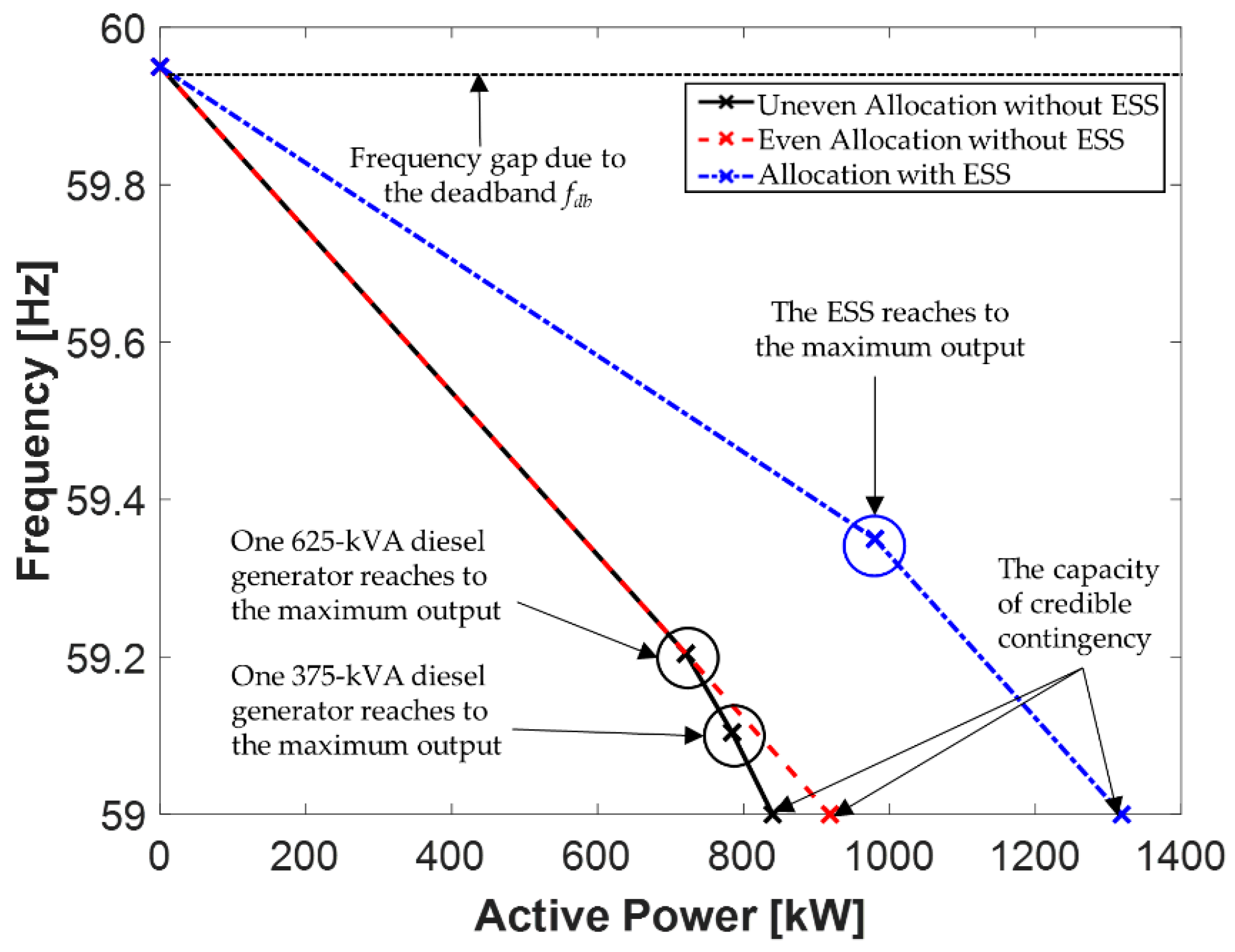
5.1. Analytical Results

Table 5 and Table 6 show the results for the case of a stand-alone microgrid without and with the ESS, respectively. The maximum penetration capacity of PV was taken as the smaller value among the values obtained in the operable capacity range of PV from Equation (5) and the magnitude of credible contingency event calculated from Section 4.1.3. Also, note that the microgrid becomes unstable if the latter is smaller than the former. From the values in Table 5 and Table 6, only stability of QSS frequency can be determined. Therefore, time-domain simulations were carried out to determine whether the microgrid was stable, considering both QSS and instantaneous frequency in Section 5.2.1 and Section 5.2.2.

The maximum penetration capacity of PV could be achieved with one 375-kVA and four 625-kVA diesel generators in Table 5. In this case (Case 1A in Table 5), the PV could be installed with the capacity of 680 kW. Thus, the penetration level was approximately 42.5%. This result was validated by comparison with three other cases (Cases 1B, 1C, and 1D in Table 5), where the PV with the same capacity was installed in Section 5.2.3. The case with three 375-kVA and three 625-kVA diesel generators was excluded because only 640 kW was allowed for the PV installation. Based on the results, Case 1D in Table 5 was selected, with the fifth highest magnitude for credible contingency. The maximum capacity of PV for the microgrid with the ESS of 400 kW is shown in Table 6. Similarly, four cases (Cases 2A–2D) were selected with the same criterion. Case 2A shows the maximum penetration level of the PV, which was 56.7% (or 906 kW for the PV). Cases 2B, 2C, and 2D were also compared with Case 2A, and the results are given in Section 5.2.3. In all cases, the maximum capacity of PV was rounded to the nearest integer since the value of ΔPV_cap was set to 1 kW.

5.2. Dynamical Simulation Results

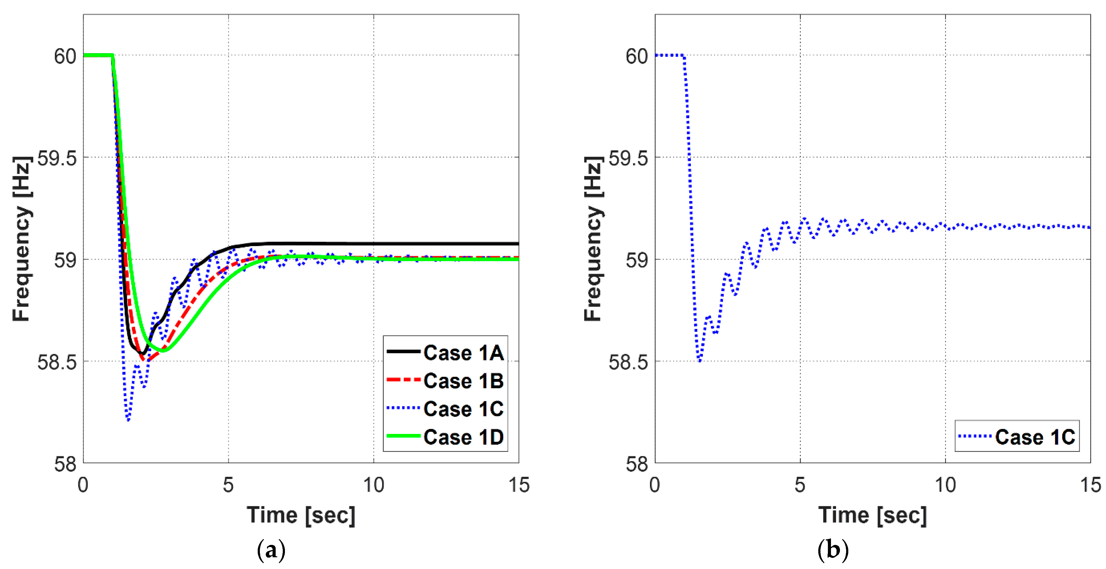
5.2.1. Frequency Responses without ESS

The time-domain simulations were performed to verify the evaluated maximum capacity of PV without ESS for each case, as shown in Figure 6. At 1 s, the power generated by the installed PV decreased from its maximum to zero. The QSS frequency for Case 1A was 59.08 Hz, while the frequency deviation calculated by the dynamic droop equation was 59.07 Hz for the contingency of 680 kW as shown in Figure 6a. For Cases 1B–1D, the system frequency decreased from its nominal value of 60 Hz to 59 Hz. Thus, it can be concluded that the QSS frequency was stable for all four cases. However, the minimum instantaneous frequency in Case 1C was 58.2 Hz, deviating beyond the required limit of 58.5 Hz. Therefore, the capacity of PV should be reduced at the last step of proposed algorithm. In Case 1C, the capacity of PV decreased from 633 kW to 533 kW considering the instantaneous frequency limit as shown in Figure 6b. Thus, the stability of both QSS and instantaneous frequency was satisfied.

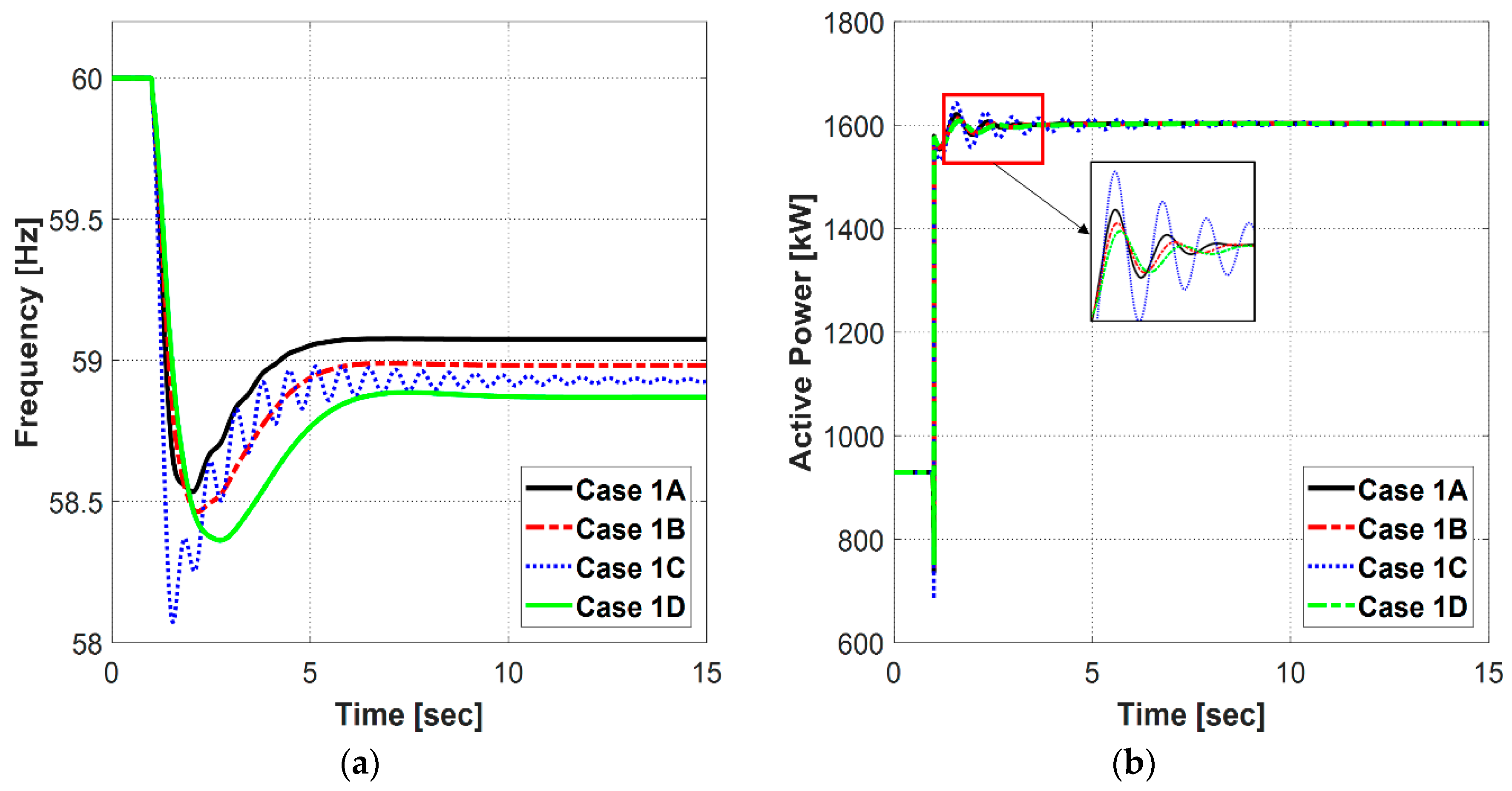
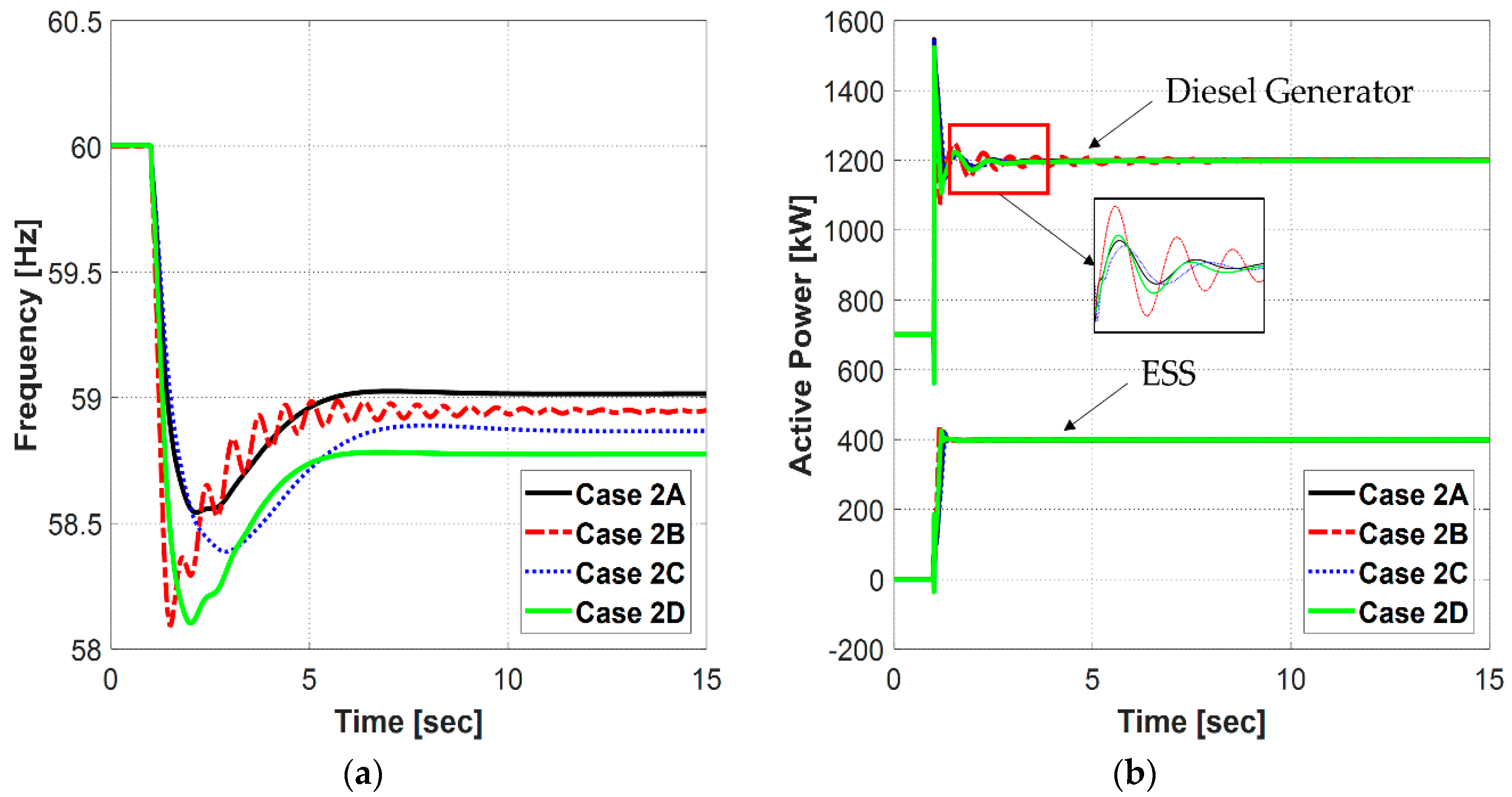
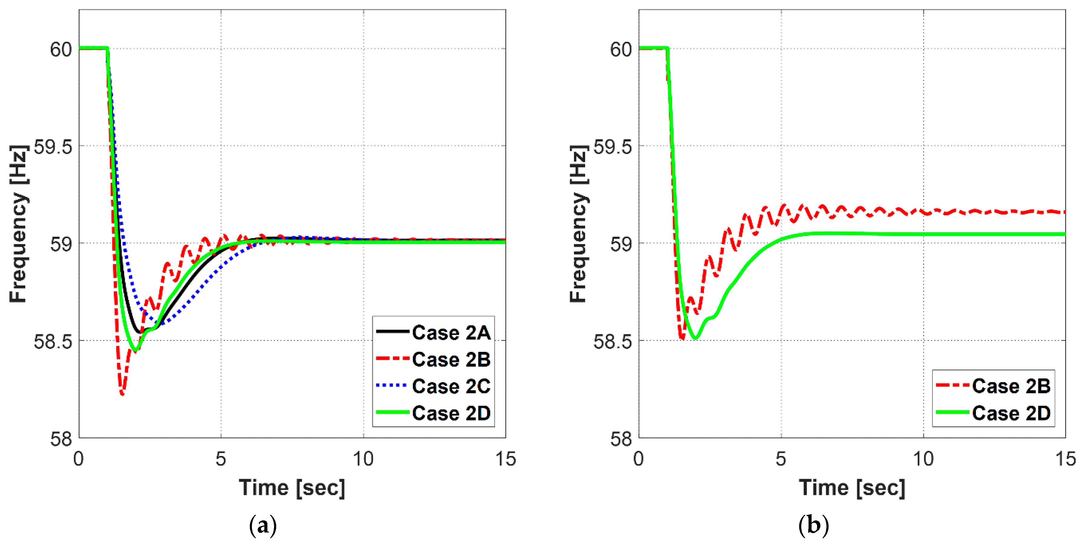
5.2.2. Frequency Responses with ESS

When the ESS is installed, the microgrid will have additional reserve power so that larger capacity of PV can be accepted. Similar to the results for Case 1A–1D in Figure 6, the microgrid with ESS kept stable operation while the system frequency decreased to 59 Hz in all four cases (Cases 2A–2D), as shown in Figure 7a. For Cases 2A–2D with the QSS frequency of 59 Hz, the frequency deviation calculated by the dynamic droop equations was 1 Hz (i.e., the Δf_m = 59 Hz) because the magnitude of the credible contingency event and the capacity of PV were almost same. Therefore, all cases ensured stability in term of the QSS frequency. However, the minimum instantaneous frequencies in both Cases 2B, and 2D deviated beyond the required limit of 58.5 Hz. To satisfy the stability of instantaneous frequency in Cases 2B and 2D, the PV capacities decreased from 874 kW to 795 kW, and from 811 kW to 800 kW, respectively, as shown in Figure 7b.

5.2.3. Maximum Capacity of PV for Entire Cases

The maximum capacity of PV for Cases 1A–1D was verified by analyzing the frequency response after the same disturbance of 680 kW, which was the maximum value of all cases in Table 5. The magnitude of disturbance was smaller than the value of credible contingency event in Case 1A. Therefore, the system frequency was stable in Case 1A since the QSS frequency after the disturbance was 59.08 Hz, which was higher than the limit of 59 Hz as shown in Figure 8a. However, the values of credible contingency event in the other three cases (Cases 1B–1D) were 665 kW, 633.3 kW, and 601.6 kW, respectively. In other words, the magnitude of disturbance was higher than the value of credible contingency event in Cases 1B–1D. As a result, both the QSS frequency and instantaneous frequency fluctuated beyond their limits of 59 Hz and 58.5 Hz, respectively, in Cases 1B–1D. The power outputs from the diesel generators increased from 920 kW to 1600 kW for each case as shown in Figure 8b. Case 1D shows the smallest oscillation after a disturbance due to its larger system inertia constant. However, the deviation of QSS frequency was also the largest, at 58.87 Hz. This result occurred because the inertia constant only influenced the minimum instantaneous frequency. In conclusion, the inertia constant is not the main index for evaluating the maximum penetration of PV, and it is, thus, only used in the last step of proposed algorithm. The results for the cases listed in Table 6 are given in Figure 9. Similar to the results for Cases 1A–1D, it can be observed from Figure 9a that the system frequency was only stable for Case 2A. In the other three cases (Cases 2B–2D), the deviations of QSS frequency were larger than the limit after the same disturbance of 906 kW, which was the maximum value of all the cases in Table 6. In addition, the output powers from the ESS increased from zero to 400 kW in all cases, as shown in Figure 9b, indicating that the full capacity of the ESS was used to compensate for the generation reduction of PV. Therefore, after a disturbance at 1 s, the ESS was unable to regulate the system frequency.

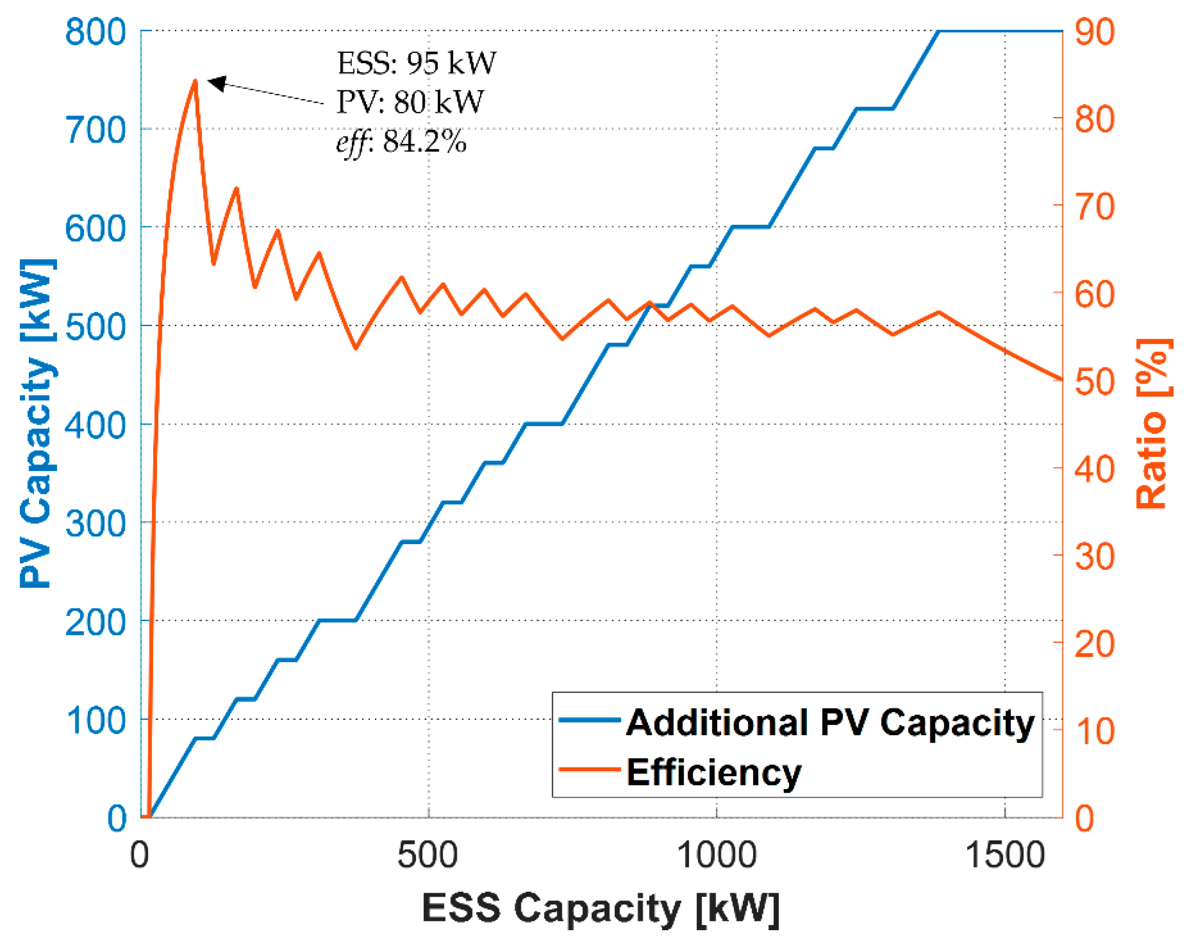
5.3. Relationship between PV and ESS

The relationship between the additional capacity of PV and the installed capacity of ESS on the practical stand-alone microgrid is analyzed in this section. It is obvious that the greater capacity of ESS led to the greater permissible capacity for PV, as shown in Figure 10. However, when the ESS is over-installed, its efficiency will decrease as follows:

$$eff=\frac{P{V}_{cap,add}}{ES{S}_{cap}}\times 100,$$

(11)

where the ESS_cap is the installed capacity of the ESS, PV_cap,add is the additional capacity of PV when the ESS is installed with the value of ESS_cap, and eff is the efficiency of ESS for the value of PV_cap,add. When the ESS is installed with 95 kW, the additional permissible capacity of PV will be 80 kW, with a maximum efficiency of 84.2%. In addition, the ESS can be optimally sized based on the capacity of planned PV for “D” island. Although the results are specified for the “D” island, the efficiency decreases as the capacity of ESS increases after the optimal point.

6. Conclusions

This paper proposed a new method for evaluating the maximum penetration capacity of a photovoltaic (PV) generator for a practical stand-alone microgrid with high renewable penetration. The credible contingency event was calculated for the microgrid using the dynamic droop equation, which incorporates the relationship between the deviation in system frequency and the size of active power disturbance in real time. By considering both quasi-steady-state (QSS) and instantaneous frequency, the maximum capacity of PV for a given number of diesel generators can be evaluated. As the result, the generation composition of microgrid can be determined to achieve the highest renewable penetration level with or without the ESS. Moreover, the relationship between the additional capacity of PV and ESS was analyzed to select the optimal size of ESS.

To verify the effectiveness of the proposed algorithm, several case studies were carried out by using both mathematical and simulation-based analyses. The results showed that the proposed evaluation method could only determine the maximum penetration capacity of PV and size of the credible contingency event in terms of QSS frequency. Therefore, time-domain simulations must be carried out to access whether the system frequency varies beyond the maximum instantaneous frequency deviation limit.

References

1. Wang, T.; O’Neill, D.; Kamath, H. Dynamic Control and Optimization of Distributed Energy Resources in a Microgrid. IEEE Trans. Smart Grid 2015, 6, 2884–2894. [Google Scholar] [CrossRef]
2. Wu, D.; Tang, F.; Dragicevic, T.; Vasquez, J.C.; Guerrero, J.M. A Control Architecture to Coordinate Renewable Energy Sources and Energy Storage Systems in Islanded Microgrids. IEEE Trans. Smart Grid 2015, 6, 1156–1166. [Google Scholar] [CrossRef]
3. Roposki, B.; Sen, P.K.; Malmedal, K. Optimum Sizing and Placement of Distributed and Renewable Energy Sources in Electric Power Distribution Systems. IEEE Trans. Ind. Appl. 2013, 49, 2741–2752. [Google Scholar] [CrossRef]
4. Van de Vyver, J.; De Kooning, J.D.; Meersman, B.; Vandevelde, L.; Vandoorn, T.L. Droop Control as an Alternative Inertial Response Strategy for the Synthetic Inertia on Wind Turbines. IEEE Trans. Power Syst. 2016, 31, 1129–1138. [Google Scholar] [CrossRef]
5. Zheng, L.; Hu, W.; Lu, Q.; Min, Y. Optimal Energy Storage System Allocation and Operation for Improving Wind Power Penetration. IET Gener. Transm. Distrib. 2015, 9, 2672–2678. [Google Scholar] [CrossRef]
6. Kim, J.; Lee, S.H.; Park, J. Inertia-Free Stand-Alone Microgrid—Part II: Inertia Control for Stabilizing DC-Link Capacitor Voltage of PMSG Wind Turbine System. IEEE Trans. Ind. Appl. 2018, 54, 4060–4068. [Google Scholar] [CrossRef]
7. Miao, L.; Wen, J.; Xie, H.; Yue, C.; Lee, W. Coordinated Control Strategy of Wind Turbine Generator and Energy Storage Equipment for Frequency Support. IEEE Trans. Ind. Appl. 2015, 51, 2732–2742. [Google Scholar] [CrossRef]
8. Teng, J.-H.; Luan, S.-W.; Lee, D.-J.; Huang, Y.-Q. Optimal Charging/Discharging Scheduling of Battery Storage Systems for Distribution Systems Interconnected with Sizeable PV Generation Systems. IEEE Trans. Power Syst. 2013, 28, 1425–1433. [Google Scholar] [CrossRef]
9. Venkataraman, S.; Ziesler, C.; Johnson, P.; Kempen, S.V. Integrated Wind, Solar, and Energy Storage: Designing Plants with a Better Generation Profile and Lower Overall Cost. IEEE Power Energy Mag. 2018, 16, 74–83. [Google Scholar] [CrossRef]
10. Knap, V.; Chaudhary, S.K.; Stroe, D.; Swierczynski, M.; Craciun, B.; Teodorescu, R. Sizing of an Energy Storage System for Grid Inertial Response and Primary Frequency Reserve. IEEE Trans. Power Syst. 2016, 31, 3447–3456. [Google Scholar] [CrossRef]
11. Majumder, R.; Chaudhuri, B.; Ghosh, A.; Majumder, R.; Ledwich, G.; Zare, F. Improvement of Stability and Load Sharing in an Autonomous Microgrid Using Supplementary Droop Control Loop. IEEE Trans. Power Syst. 2010, 25, 796–808. [Google Scholar] [CrossRef]
12. Zhang, F.; Meng, K.; Xu, Z.; Dong, Z.; Zhang, L.; Wan, C.; Liang, J. Battery ESS Planning for Wind Smoothing via Variable-Interval Reference Modulation and Self-Adaptive SOC Control Strategy. IEEE Trans. Sustain. Energy 2017, 8, 695–707. [Google Scholar] [CrossRef]
13. Liu, Y.; Du, W.; Xiao, L.; Wang, H.; Cao, J. A Method for Sizing Energy Storage System to Increase Wind Penetration as Limited by Grid Frequency Deviations. IEEE Trans. Power Syst. 2016, 31, 729–737. [Google Scholar] [CrossRef]
14. Wang, X.; Yue, M.; Muljadi, E.; Gao, W. Probabilistic Approach for Power Capacity Specification of Wind Energy Storage Systems. IEEE Trans. Ind. Appl. 2014, 50, 1215–1224. [Google Scholar] [CrossRef]
15. Sun, C.; Liu, D.; Wang, Y.; You, Y. Assessment of Credible Capacity for Intermittent Distributed Energy Resources in Active Distribution Network. Energies 2017, 10, 1104. [Google Scholar] [CrossRef]
16. NERC Reliability Guideline—Primary Frequency Control. 2015. Available online: https://www.nerc.com/comm/OC/Reliability Guideline DL/Primary_Frequency_Control_final.pdf (accessed on 28 January 2019).
17. Guerrero, J.M.; Vasquez, J.C.; Matas, J.; Vicuna, L.G.d.; Castilla, M. Hierarchical Control of Droop-Controlled AC and DC Microgrids—A General Approach Toward Standardization. IEEE Trans. Ind. Electron. 2011, 58, 158–172. [Google Scholar] [CrossRef]
18. Turbine-Governor Models Standard Dynamic Turbine-Governor Systems in NEPLAN Power System Analysis Tool. 2015. Available online: https://www.neplan.ch/wp-content/uploads/2015/08/Nep_TURBINES_GOV.pdf (accessed on 22 March 2019).
Figure 1. Frequency response of a stand-alone microgrid after a disturbance.
Energies 12 01445 g001
Figure 2. Flowchart of the proposed algorithm.
Energies 12 01445 g002
Figure 3. Dynamic droop curves for the microgrid with three different power allocation strategies.
Energies 12 01445 g003
Figure 4. One-line diagram of a stand-alone microgrid in South Korea.
Energies 12 01445 g004
Figure 5. DEGOV1 diesel governor model.
Energies 12 01445 g005
Figure 6. Frequency responses without energy storage system (ESS): (a) after credible contingency based on the quasi-steady-state (QSS) frequency (Cases 1A–1D); (b) after credible contingency based on the instantaneous frequency (Case 1C).
Energies 12 01445 g006
Figure 7. Frequency responses with ESS: (a) after credible contingency based on the QSS frequency (Cases 2A–2D); (b) after credible contingency based on the instantaneous frequency (Case 2B and 2D).
Energies 12 01445 g007
Figure 8. Results after the photovoltaic (PV) generation decreased from 680 kW to zero for Cases 1A–1D: (a) frequency response; (b) power output from the diesel generators.
Energies 12 01445 g008
Figure 9. Results after the PV generation decreased from 906 kW to zero for Cases 2A–2D: (a) frequency response; (b) power output from the diesel generators and the ESS.
Energies 12 01445 g009
Figure 10. Additional capacity and ratio of the PV when the ESS is installed.
Energies 12 01445 g010