Article

Photovoltaic Power Converter Management in Unbalanced Low Voltage Networks with Ancillary Services Support

by
Fermín Barrero-González
1,*,
Victor Fernão Pires
2,
José L. Sousa
3,
João F. Martins
4,
María Isabel Milanés-Montero
1,
Eva González-Romera
1 and
Enrique Romero-Cadaval
1
1
School of Industrial Engineering, University of Extremadura, 06006 Badajoz, Spain
2
INESC-ID and Setúbal School of Technology, Polytechnic Institute of Setúbal, 2910-761 Setúbal, Portugal
3
INESC Coimbra and Setúbal School of Technology, Polytechnic Institute of Setúbal, 2910-761 Setúbal, Portugal
4
Faculty of Sciences and Technology, Nova University of Lisbon, 2829-516 Caparica, Portugal
*
Author to whom correspondence should be addressed.
Energies 2019, 12(6), 972; https://doi.org/10.3390/en12060972
Submission received: 22 February 2019 / Revised: 6 March 2019 / Accepted: 9 March 2019 / Published: 13 March 2019
(This article belongs to the Special Issue Power Electronic Systems for Efficient and Sustainable Energy Supply)

Abstract

:
The proliferation of residential photovoltaic (PV) prosumers leads to detrimental impacts on the low-voltage (LV) distribution network operation such as reverse power flow, voltage fluctuations and voltage imbalances. This is due to the fact that the strategies for the PV inverters are usually designed to obtain the maximum energy from the panels. The most recent approach to these issues involves new inverter-based solutions. This paper proposes a novel comprehensive control strategy for the power electronic converters associated with PV installations to improve the operational performance of a four-wire LV distribution network. The objectives are to try to balance the currents demanded by consumers and to compensate the reactive power demanded by them at the expense of the remaining converters’ capacity. The strategy is implemented in each consumer installation, constituting a decentralized or distributed control and allowing its practical implementation based on local measurements. The algorithms were tested, in a yearly simulation horizon, on a typical Portuguese LV network to verify the impact of the high integration of the renewable energy sources in the network and the effectiveness and applicability of the proposed approach.

1. Introduction

1.1. Generally Known Information about the Topic

Due to reduced costs, government incentives and increased community awareness of environmental problems, installed power from distributed energy sources, or micro- and mini-generation plants has increased. Among low-voltage (LV) networks, rooftop photovoltaic (PV) systems represent a higher percentage. With the recent legislation, a new regime has appeared: the so called self-consumption scheme. In this regime, the electrical energy produced is used primarily to supply on-site loads, while any excess of energy can be sold to the utility. When production is not sufficient to satisfy consumption, the energy deficit is supplied by the utility. Therefore, the classical consumer is becoming a prosumer, defined as a combination of an energy consumer and producer, interacting bi-directionally with the distribution grid [1]. The proliferation of residential PV prosumers leads to detrimental impacts on the network operation. Amongst the reported problems, the most relevant ones are voltage regulation and voltage imbalance.
To properly understand these impacts, one must take into account the network structure. In Europe (and in many other parts of the world), LV networks are usually three-phase, four-wire systems, supplied by three-phase transformers, forming radial network structures [2,3,4]. Most of the houses are single-phase loads and are supplied connecting them to one of the three phases and neutral, while larger houses have three-phase connections. Originally, the grid was designed to operate with a unidirectional power flow, and distribution systems are operated on the assumption that the energy flows are unidirectional, going from upstream to downstream where the loads are placed. In this situation, the typical voltage profile is decreasing from the transformer, at the beginning of the network, to the consecutive supplied loads.
Generally, PV panels are connected to the network by means of an electronic power converter, which is designed to obtain the maximum solar energy and to inject it to the network [5]. As this type of energy has intermittent characteristics, when its penetration is reduced, there are no negative impacts on the network. However, in a context including numerous prosumers, in high PV production periods, there is a possibility of significant reverse power flow and, mainly on cloudy days, serious voltage fluctuations may occur. This may cause overloading and violation of power quality standards such as surges above limit values [6,7,8]. The described LV network has an inherently unbalanced behaviour, due to the random load distribution between phases and also due to uneven consumption. The increasing installation of single-phase rooftop PV unit and the fact that they are installed at random locations and have different ratings, contributes to worsening the imbalance problem [9]. Besides, as a consequence of the unbalanced current flowing through the network, current flows through the neutral wire. The flow of this current through the neutral grounding impedances will cause a rise of the neutral-to-ground voltage (NGV), which can damage sensitive electronic and computing equipment due to the common-mode noise effect. Limits to imbalances are imposed by the standards, as in EN50160 [10], where a limit value of 2% is indicated for the negative-sequence to positive-sequence voltage ratio.
Traditionally, the voltage regulation issue has been addressed by the utility, mainly by means of the operation of tap-changing transformers, voltage step regulator and switching capacitors. On the other hand, the utilities try to minimize the imbalance problem by manually changing the customer single-phase connections to achieve a more balanced distribution of the loads, resizing the neutral conductor or improving the grounding system. Apart from the possible increase in the installation costs, the inherent rapid variability of PV power would make it difficult for these basically “static” mitigation techniques to compensate the combined effect of load and PV.

1.2. Prior Studies’ Historical Context to the Research

Recent approaches to overcome the voltage regulation and the imbalance problems in LV networks with high PV power penetration involve inverter-based solutions. Taking into account the support that these systems can give to the electric energy networks, in the context of smart grids, these converters have been designated as smart inverters.
Some papers address the voltage regulation problem by means of the reactive power control [11,12,13]. These studies, in many cases, are based on a balanced network model which, however, is not the case in LV networks. Moreover, PV control strategies based only on reactive power control, which is not an effective approach in distribution networks with high R/X ratios, are relatively common. Regarding voltage imbalance, some work has been presented in which the three-phase inverters inject current in the network that can be balanced or not, according to the load [14,15]. More recently, in [16], the residential loads are transferred from one phase to another to minimize voltage imbalances along the feeder. The concept of real power curtailment is used in [17,18]. A hierarchical optimisation strategy with coverage from the substation zone to the LV feeder is proposed in [19]. A hierarchical control structure is proposed to reduce power oscillations under unbalanced voltage in [20]. Community energy storage is applied for the mitigation of the neutral current in [21].
Almost all previous studies are based on centralized control and, therefore, they are generally complex and need local measurement and communication between a centralized master controller and the prosumers [22]. By contrast, in a distributed control scheme, control actions of each prosumer are decided based on local measurements [23,24,25]. Though, these studies do not deal with voltage imbalance, which is especially helpful for a more suitable practical implementation in existing networks.
Another problem in power grids is the existence of current harmonics. Thus, in order to mitigate this problem, work has also been carried out, where the possibility of the smart inverter to have a parallel mode of operation as an active power filter is verified [26,27,28,29]. In this way, it will be possible to attenuate those harmonics, allowing the improvement of the quality of the voltage waveform [30,31].

1.3. Hypothesis and an Overview of the Results

The mentioned previous studies provide a global perspective for the convenience to address a different approach. Thereby, this paper proposes a novel comprehensive control strategy for the power electronic converters associated with the PV installations to improve the operational performance of a four-wire LV distribution network. The proposed strategy will balance the currents demanded by consumers and compensate their reactive power, using the remaining capacity of the PV converters. The strategy is implemented in each consumer installation, constituting a decentralized distributed control and allowing its practical implementation with local measurement.
The simulation of a case study addresses several operating regimes, such as: (a) only generation; (b) generation and imbalance compensation and (c) generation with imbalance and reactive power compensation. These various cases are analysed considering the highest and lowest solar radiation days.

1.4. Article Organization

The rest of this paper is organized as follows: Section 2 reviews the typical PV inverter topology and the fundamental ideas of its control system. Section 3 presents the proposed control strategy describing the algorithm for voltage imbalance combined with reactive power compensation. Section 4 shows the test network and the load and generation profiles used to simulate the strategies; and analyses and discusses the results in several cases or scenarios. Section 5 concludes the paper.

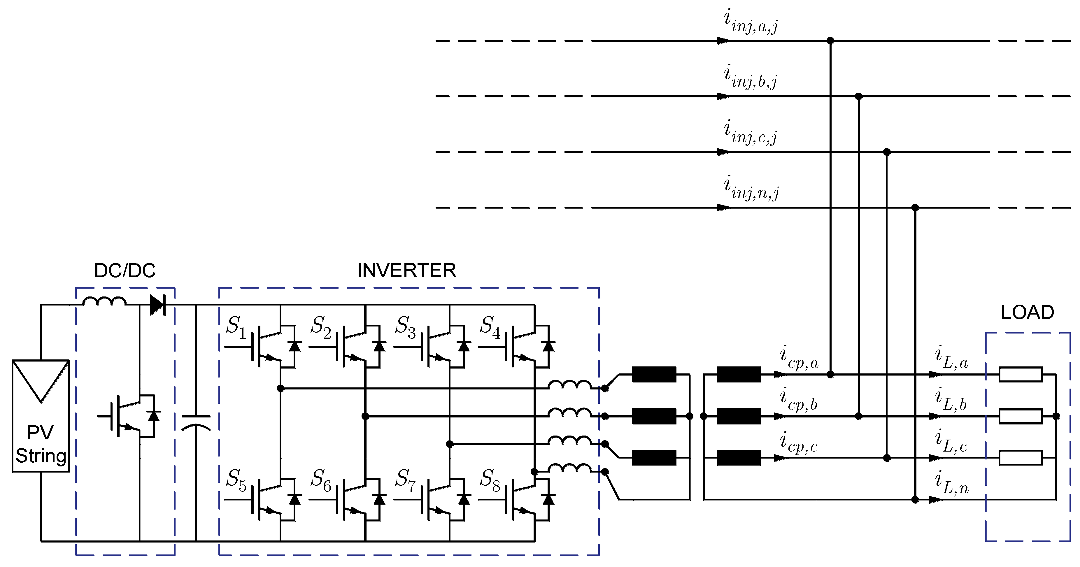
2. PV Inverters Topology and Control

A three-phase PV system transfers the produced active power to the network evenly through the use of three-phase three-leg inverter topology. However, this topology does not allow compensating for imbalance in the network resulting from unbalanced three-phase loads and the existence of single-phase consumers. To achieve the balance behaviour, the solution resides in the use of three-phase four-leg Voltage Source Inverter (VSI) (Figure 1), to access to the neutral conductor [32]. These inverters, when associated with adequate control systems, have advanced functions allowing network assistance (ancillary services).
The control strategy is the part of the current controlled VSI control system in charge to produce the reference signals for the currents, that have to be generated by the power converter (icp,a, icp,b, icp,c), taking as inputs the actual variables measurements. These references are taken as inputs to the switching signal generator, which, by means of some type of control, as dead-beat or hysteresis band control, generates the electronic devices gate pulses.
In LV networks, the typical control strategy for PV converters tries to extract the maximum energy from the panels (the DC side), usually by means of a Maximum Power Point Tracking (MPPT) algorithm, this power is then injected it into the network (the AC side), typically in balanced form and with unity power factor [5].
Using the 4-leg topology and a suitable control strategy, the PV systems may provide novel auxiliary services that appear to be more interesting for LV networks: mitigation of imbalance and voltage control support. Thus, on the one hand, the current injected by the three-phase PV system converter will be higher in the phase with higher load and lower in the others, so that the association of the inverter with the load demand currents from the grid are as balanced as possible. And even more, the three-phase converters installed in the same feeder may compensate the imbalances introduced by the single-phase loads and their respective PV single-phase converters. On the other hand, PV systems also allow the exchange of reactive power to contribute to voltage regulation. In order to avoid increasing the converters rated power, the reactive power absorbed/injected by the power converter must take into account the active power generated by the solar panel. Being S and P the inverter’s apparent and active power produced, respectively, the proposed algorithms will limit the reactive power Q to be injected according to the following expression: Q S 2 P 2 . This means that when the solar panel is at its maximum power, the available reactive power of the electronic converter is zero. The limit of the reactive power increases with the decrease of the active power supplied by the solar panel. The maximum reactive power available occurs when the active power supplied by the panel is zero. It should also be pointed out that the inverter must be sized taking into consideration the allowed imbalance compensation. At the limit, all the generated PV power would be injected into the grid by one phase. Thus, each of the inverter legs should be sized to support the maximum generated PV power. However, since the inverter is also used to provide ancillary services, as in this case the reactive power compensation, that oversize can be used for that support.

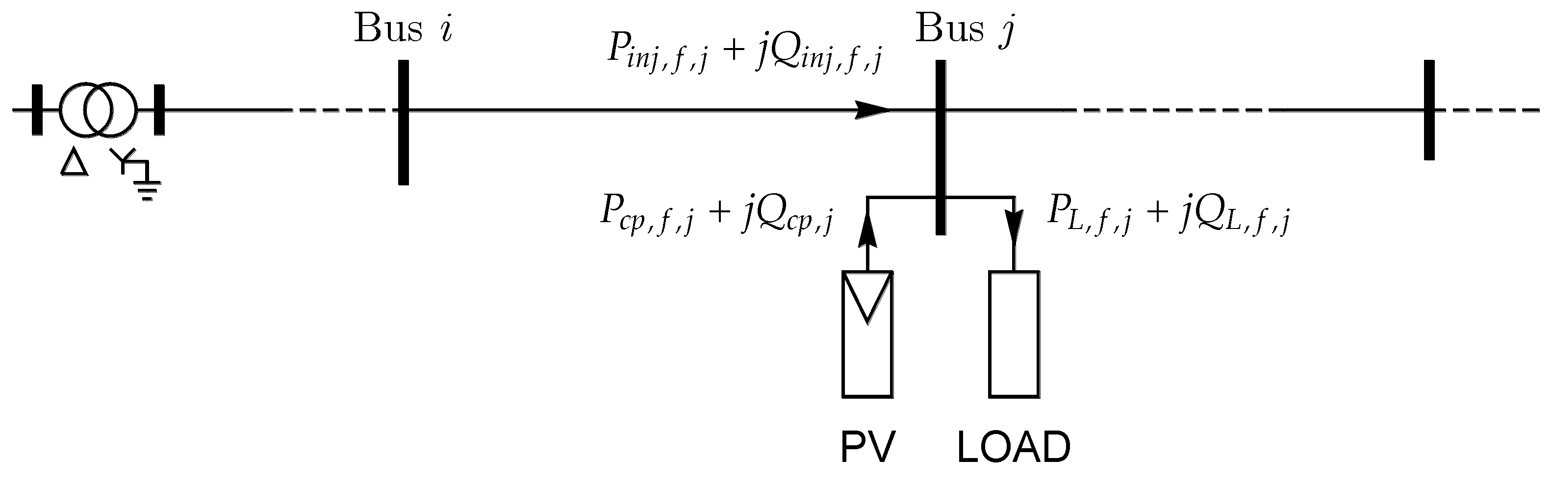
3. Proposed PV Inverter Control Strategy

Figure 2 shows a generic bus j of the radial LV network under study. It can be observed the active and reactive power flows in each phase f (a, b ,c) that will be used hereinafter, along with its reference directions: the injected power at the bus ( S i n j , f , j = P i n j , f , j + j Q i n j , f , j ), the power demanded by the load S L , f , j = P L , f , j + j Q L , f , j and the power supplied by the PV S c p , f , j = P c p , f , j + j Q c p , f , j . The proposed algorithm will define for each PV inverter the active and reactive power set points for each phase ( P c p , f , j and Q c p , f , f , in order to balance the network and to improve the voltage profile. These set-point values will be used to produce the aforementioned reference currents for the VSI.

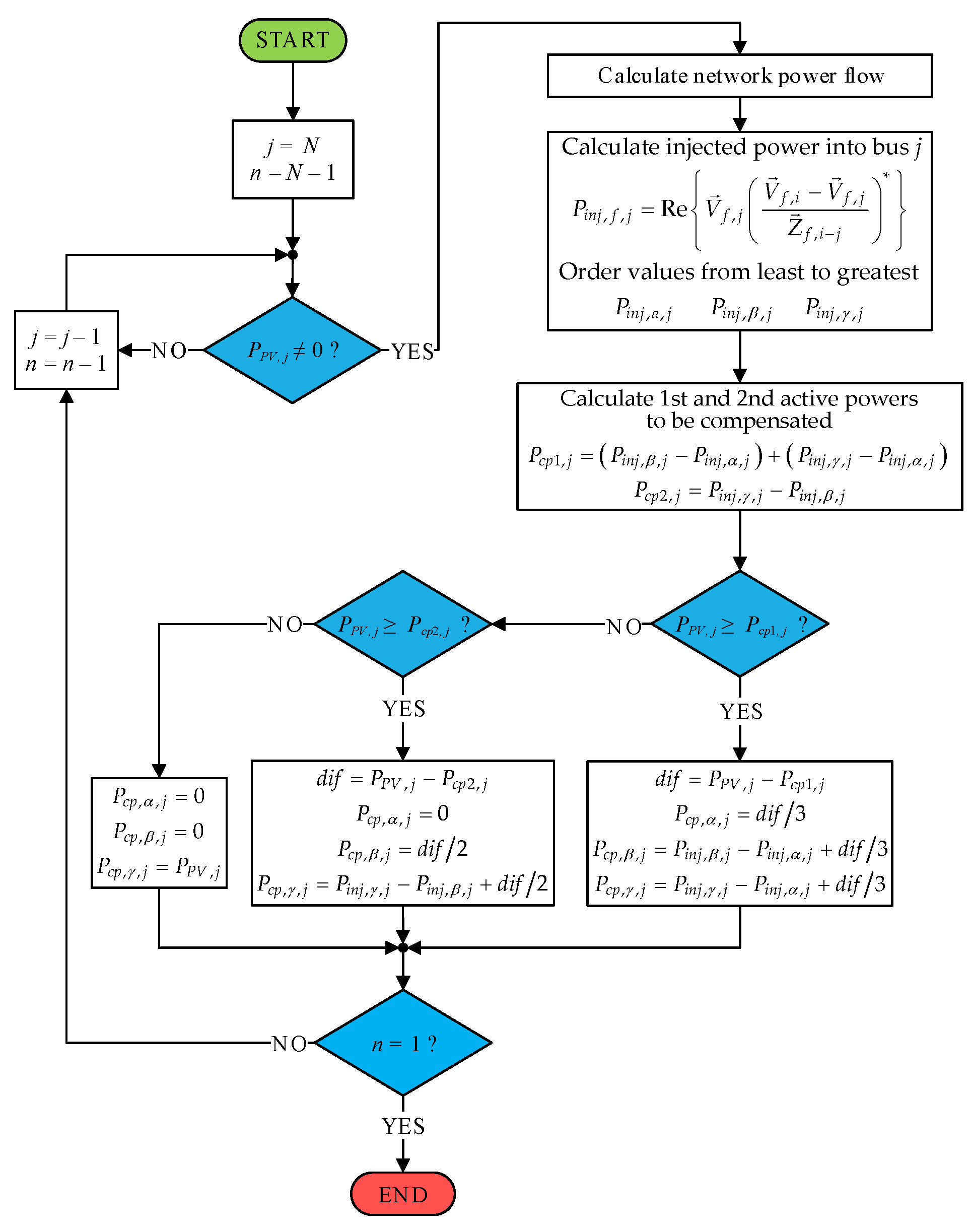
3.1. Proposed Imbalance Compensation Algorithm

The algorithm for phase imbalance compensation consists of injecting more active power from PV in the phases with higher consumption. Besides balancing the phases in the network, this procedure also helps regulating the voltage.
The procedure begins with the verification of the existence of three-phase PV generation in the farthest node N, seen from the MV/LV transformer. If this is the case, the active power flowing to the downstream bus j in each phase f, P i n j , f , j is determined:
P i n j ,   f ,   i = Re { V f ,   j ( V f ,   i V f ,   j   Z f ,   i j ) * } ,
where V f , i and V f , j are the phase f voltage phasors (in V) at the adjacent buses i and j, respectively; and Z f , i j is the phase f impedance (in Ω ) of the line between buses i and j.
In order to calculate these voltages, a power flow program adapted to LV networks is used [33]. Load values are data (in a first step PV generation is not considered), voltage at bus 1 is set to 1 pu. and the power flow program gives the bus voltages. The compensation algorithm, as it will be explained in the following paragraphs, will calculate the compensation powers progressively from the farthest bus to the transformer bus. In each step, the power flow program gives the updated bus voltages. This procedure is necessary for simulation purposes, to demonstrate the proper operation of the proposed strategy. However, in a practical implementation of this control strategy on power electronics converters, P i n j , f , j would not be calculated by Equation (1), but it would be directly measured at bus j, which justify the advantageous feature (mentioned in the introduction) that the control actions are based only on local measurement.
At each bus, the phase with the lowest power value is designated by α, its value is P i n j , α , j = min ( P i n j , f , j ) , the following one is designated by β, its value is P i n j , β , j and the phase with the highest value is designated by γ, its value is P i n j , γ , j . Then, the first total three-phase active power to be compensated at the bus j is calculated as:
P c p 1 , j = ( P i n j , β , j P i n j , α , j ) + ( P i n j , γ , j P i n j , α , j ) .
The next step is to verify if the system is able to compensate the three phases, that is, if the three-phase production at bus j, P P V , j , is greater than or equal to the total power to compensate, i.e., if it is P P V , j P c p 1 , j . In that case, the difference between these two powers is calculated d i f = P P V , j P c p 1 , j . Then, the compensation power for each phase α, β, γ at the bus j are obtained in the following way:
P c p ,   α ,   j = d i f / 3
P c p , β , j = P i n j , β , j P i n j , α , j + d i f / 3
P c p , γ , j = P i n j , γ , j P i n j , α , j + d i f / 3
If the system cannot compensate the three phases, then it is verified if it is possible to compensate the two phases with the highest injected powers, β and γ. To achieve this, the second total active power to be compensated at the bus j is calculated as:
P c p 2 ,   j = P i n j ,   γ ,   j P i n j ,   β ,   j
Next, this value is compared to the three-phase production at bus j, i.e., it is verified if P P V , j P c p 2 , j . If so, the difference between these two power values d i f = P P V , j P c p 2 , j is calculated. Then, the compensation powers for each phase at the bus j are obtained in the following way:
P c p , α , j = 0
P c p , β , j = d i f / 2
P c p , γ , j = P i n j , γ , j P i n j , β , j + d i f / 2
Finally, if P P V , j < P c p 2 , j , there is not enough PV generation to compensate phases β and γ, then the total available power is applied to phase γ. Therefore, in this case, the compensation power for each phase at the bus j are:
P c p , α , j = 0             P c p , β , j = 0             P c p , γ , j = P P V , j
The process is repeated from the farthest bus until the transformer bus. Figure 3 shows the flowchart of the described algorithm.
When the load changes, the algorithm must be run again. As said before, the process starts without considering the PV sources and calculating the compensation powers progressively from the farthest node to the transformer node. Therefore, one load state will not have influence on the next load state.

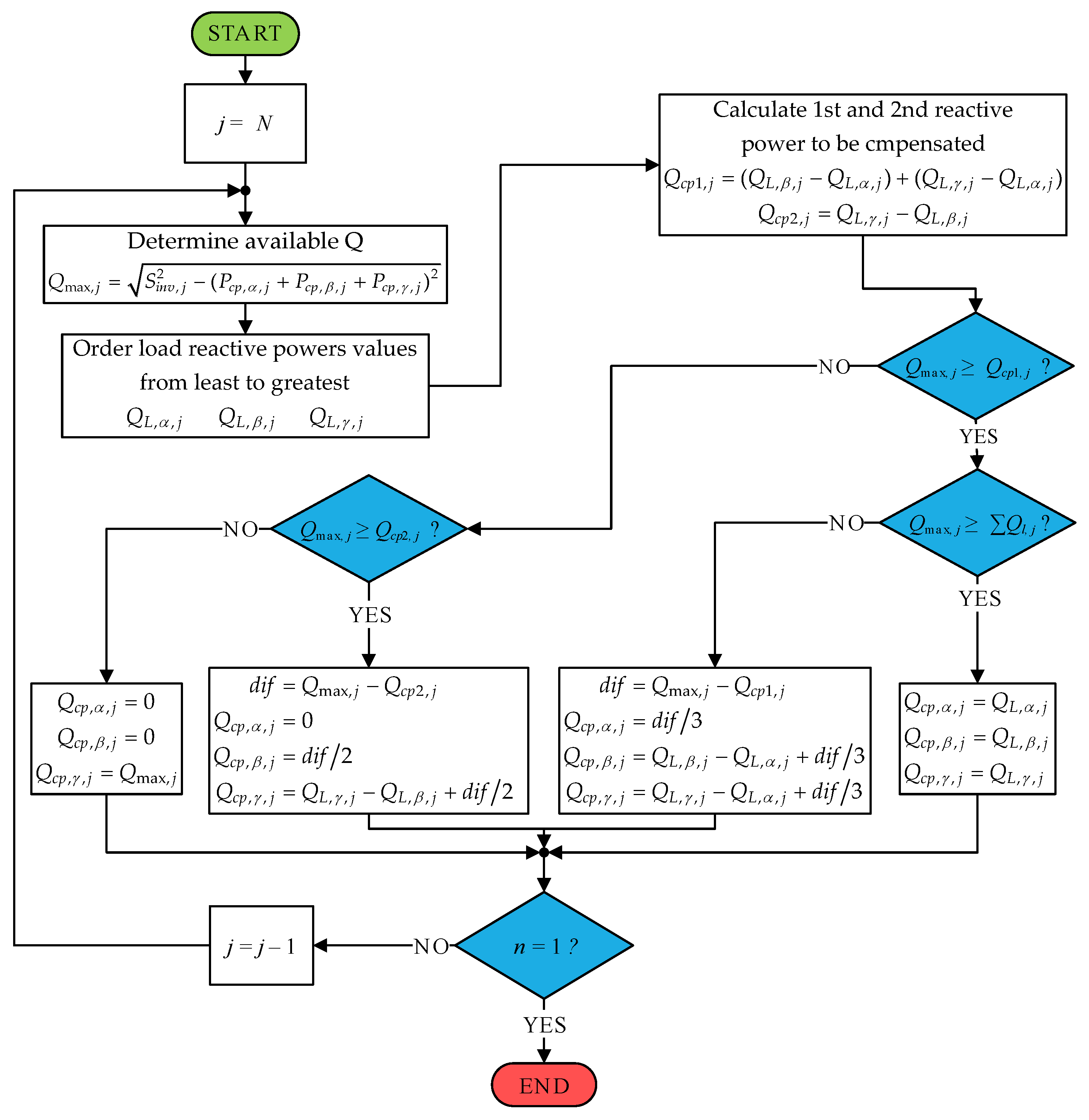
3.2. Proposed Reactive Power Compensation Algorithm.

This section presents an algorithm for load reactive power compensation, taking into account the PV converters capacity. An inductive load will be assumed, as usual case, and then reactive power demanded QL is always positive. The algorithm also starts on the farthest bus seen from the MV/LV transformer.
The reactive power available for compensation, Qmax,j, is determined from the inverter nominal power, Sinv,j, and the active power supplied into each phase of the bus, i.e.,:
Q max , j = S i n v ,   j 2 ( P c p ,   α ,   j + P c p ,   β ,   j + P c p ,   γ ,   j ) 2 .
Similarly as it was done in the previous algorithm, the phase with the lowest absolute value is designated by α, its value is Q L , α , j = min ( Q L , f , j ) , the following is designated by β, its value is Q L , β , j and the phase with the highest value is designated by γ, its value is Q L , γ , j . Then, the first and second total three-phase reactive power to be compensated at the bus j are calculated as follows:
Q c p 1 , j = ( Q L , β , j Q L , α , j ) + ( Q L , γ , j Q L , α , j ) .
Q c p 2 , j = Q L , γ , j Q L , β , j .
The next step is to verify if the system is able to compensate for the three phases, that is, if the three-phase reactive power available for compensation at bus j, Qmax,j, is greater than or equal to the total reactive power to compensate, i.e., if it is Qmax,jQcp1,j. In that case, the difference between these two powers is calculated dif = Qmax,jQcp1,j. If besides that, difQL,α,j + QL,β,j + QL,γ,j holds true, then the system is able to produce the reactive power that the load demands and the compensation power for each phase α, β, γ at the bus j, are obtained as:
Q c p ,   α ,   j = Q L ,   α ,   j
Q c p ,   β ,   j = Q L ,   β ,   j
Q c p ,   γ ,   j = Q L ,   γ ,   j
If the condition difQL,α,j + QL,β,j + QL,γ,j is not satisfied, the system cannot cancel out the reactive power of all load phases, but it can balance them according to:
Q c p ,   α ,   j = d i f / 3 .
Q c p ,   β ,   j = Q L ,   β ,   j Q L ,   α ,   j + d i f / 3 .
Q c p ,   γ ,   j = Q L ,   γ ,   j Q L ,   α ,   j + d i f / 3 .
If Qmax,j < Qcp1,j, the system cannot balance all three phases, then it is verified if it is possible to balance the two phases with the highest power, β and γ. To achieve this, it is verified if Qmax,n > Qcp2,n. If so, the difference between these two power values is calculated dif = Qmax,jQcp1,j. Then, the compensation powers for each phase, at the bus j, are obtained in the following way:
Q c p ,   α ,   j = 0 .
Q c p ,   β ,   j = d i f / 2 .
Q c p ,   γ ,   j = Q L ,   γ ,   j Q L ,   β ,   j + d i f / 2 .
Finally, if Qmax,j < Qcp2,j, there is not enough reactive power to compensate phases β and γ, then the total available reactive power is used for phase γ. Therefore, the compensation power for each phase will be:
Q c p , α , j = 0             Q c p , β , j = 0             Q c p , γ , j = Q max , j
The process is repeated from the transformer to the farthest bus. Figure 4 shows the flowchart of the algorithm.

4. Simulation Results and Analysis
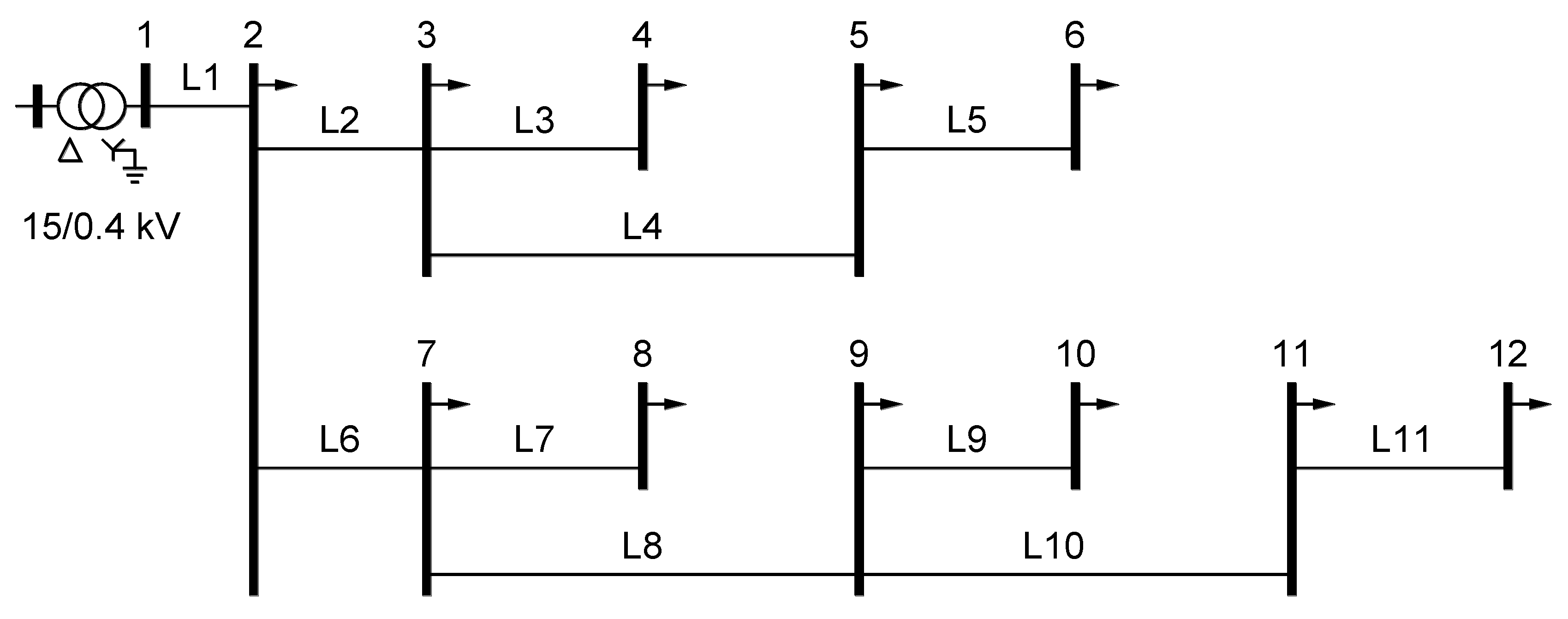
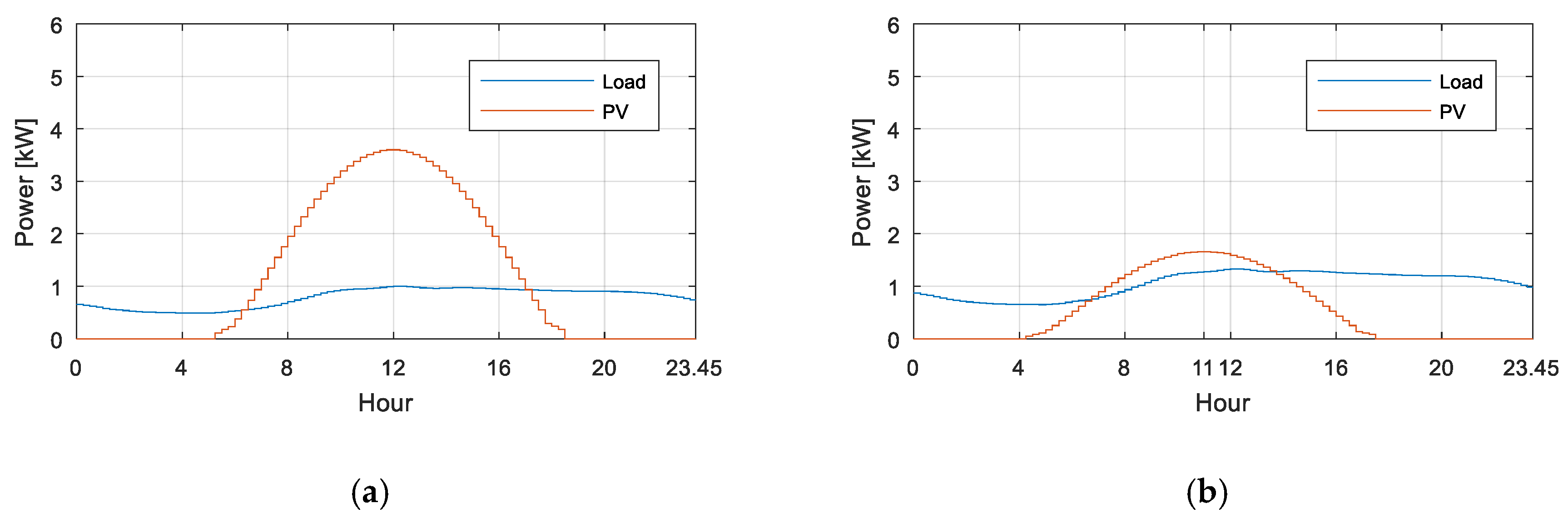
4.1. Test Network

For the analysis of the impact of decentralized photovoltaic systems, a network with 12 buses connected to a 15/0.4 kV transformer is used, which is represented in Figure 5. In total there are 240 consumers, 105 single-phase and 135 three-phase, associated in 12 groups. Line impedances (resistance R and reactance X) are given in Table 1.
A level of consumption (ranging from 3000 to 10,000 kWh/year) and contracted three-phase power normalized in Portugal (10.35, 13.8, 17.25 and 20.7 kVA) were randomly assigned. Load profiles for each consumer were obtained from estimated annual profiles for 15 min intervals, available at ERSE [34]. In addition, in the case of single-phase consumers, a phase of the network was also randomly assigned. The buses have a mixture of single- and three-phase connections; therefore the load is inherently unbalanced.
Through the PVGIS simulator [35], data on solar radiation were obtained. For this it was necessary to indicate the location of the network, the PV panels slope and their azimuth. For the present case, it was considered that all consumers had panels with 30° slope and 0° azimuth and that they were located in Lamego, Portugal, coordinates 41°05′00″N 7°52′00″O. The PV modules used are the same for all consumers and have a performance ratio of 19.7% and an area of 11.72 m2 for each group of modules that make 1 kW. The number of panels was established so that the annual energy produced had a value close to but less than the value of the annual energy consumption. Figure 6 presents, for one of the prosumers, the load profile and the PV generation profile for every hour, in the days with highest and lowest radiation along a year.

4.2. Simulated Case Studies

The network analysis considers four distinct case studies that correspond to the following scenarios:
  • Scenario 0: No PV production;
  • Scenario 1: PV production, no imbalance compensation and no reactive power compensation;
  • Scenario 2: PV production, imbalance compensation and no reactive power compensation;
  • Scenario 3: PV production, imbalance and reactive power compensation.
The simulations were carried out for each scenario during a whole year, although the presented results, as representative samples, correspond to the days of total highest and lowest radiation along a year. In the first case, the production peak occurs at 12:00 h and in the second case at 11:00 h, so these will be the moments to evaluate. These two hours are denominated Peak-H and Peak-L hours, respectively.
The results were obtained through the implementation of the developed algorithms, previously presented, in the MATLAB R2017a environment. The power flow calculations were carried out by means of a software specifically developed for this task, based on the Backward-Forward Sweep (BFS) model, which is based on the power sum method but modified in order to consider the neutral conductor [3,35].
Two radial branches (from Figure 5) are considered to show the simulation results adequately: branch B1 constituted by lines L1, L2, L4 and L5, comprising buses 1, 2, 3, 5 and 6; and branch B2 constituted by lines L1, L6, L8, L10 and L11, comprising buses 1, 2, 7, 11 and 12. Figures 7, 9, 11 and 13 show the phase-to-neutral voltages at each bus; and Figures 8, 10, 12 and 14 show the line losses per phase. In all the cases, these variables are displayed for Peak-H and Peak-L hours.

4.3. Scenario 0. No Photovoltaic Production

The first scenario serves as a baseline scenario. As expected in Figure 7, it is possible to verify that the voltage value tends to decrease towards the downstream buses. On the day of lowest radiation, there is a greater voltage drop since consumption is higher (winter). It is also possible to verify through the voltage profiles of the various phases, the voltage imbalance in the network due to the unbalanced loads. It should be noted that at any point in the network, the voltage drop is less than 0.1 p.u.
As can be seen in Figure 8, it is also possible to verify that the losses in the day of lower radiation are higher, which is justified by the fact that consumption is higher on that day (winter) along with no power generation.

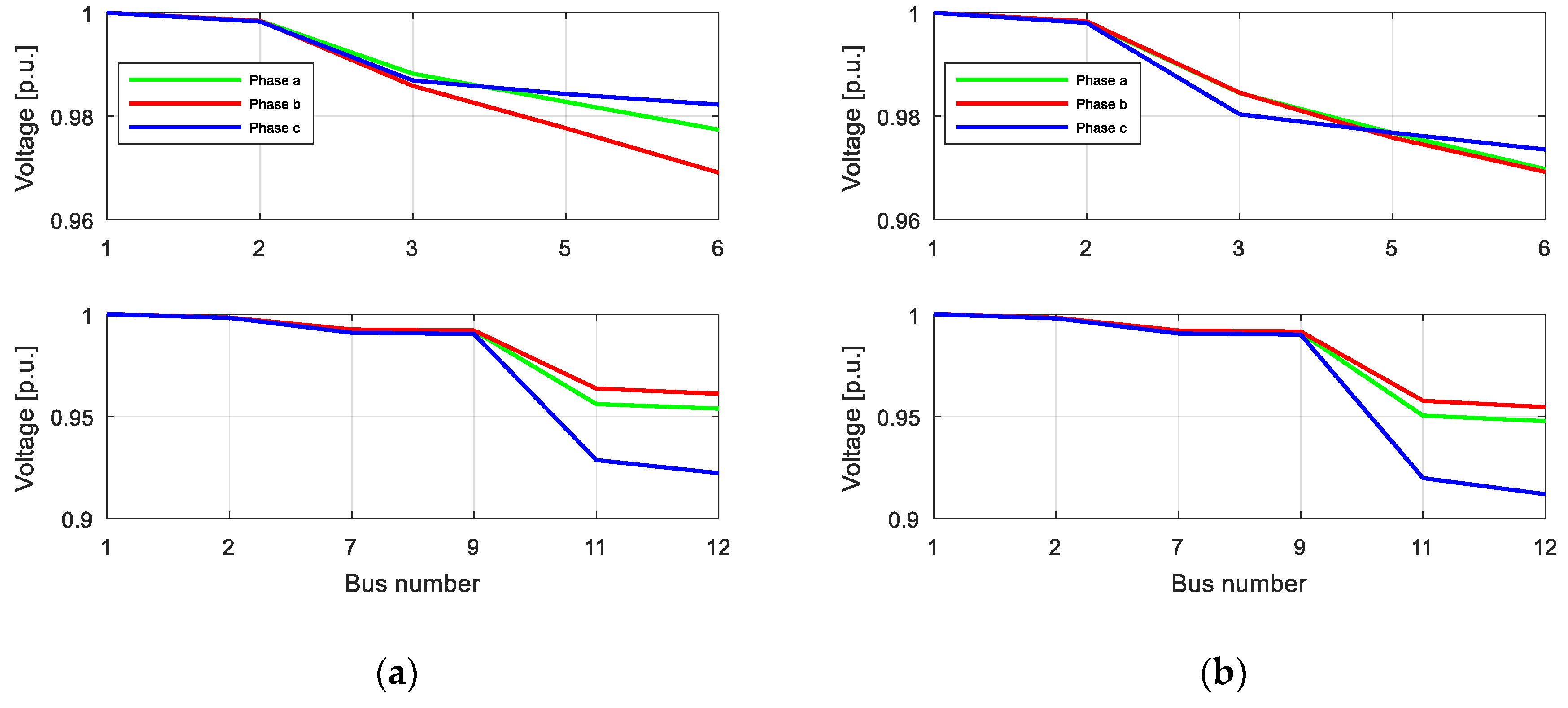
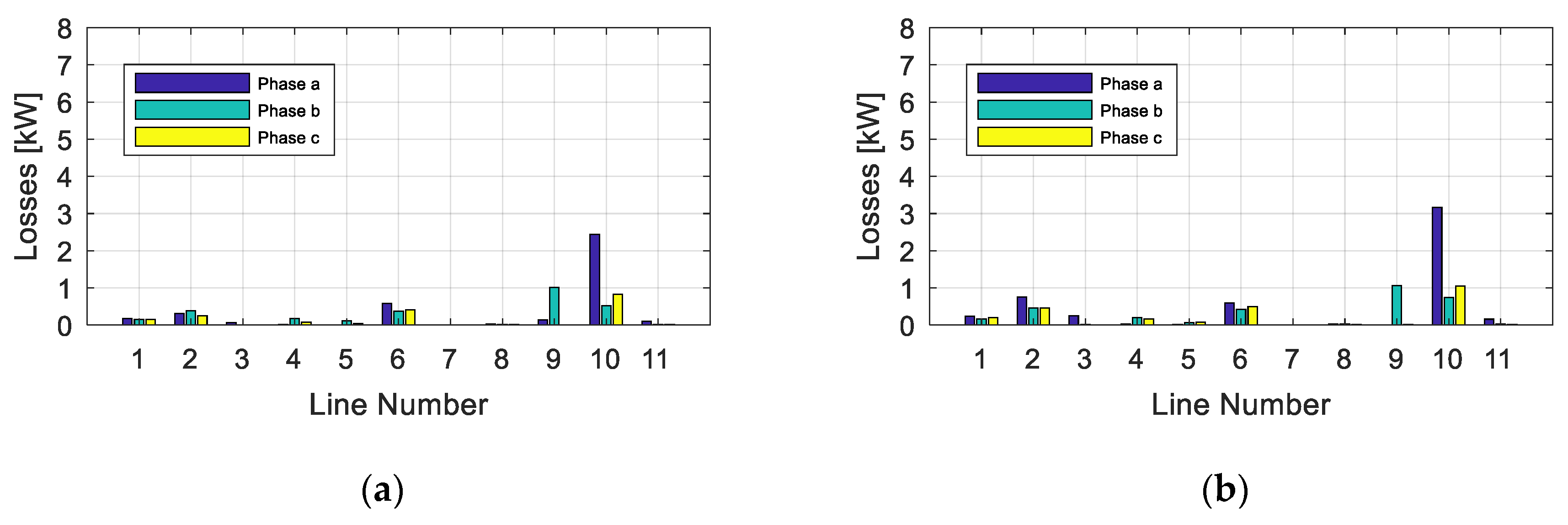
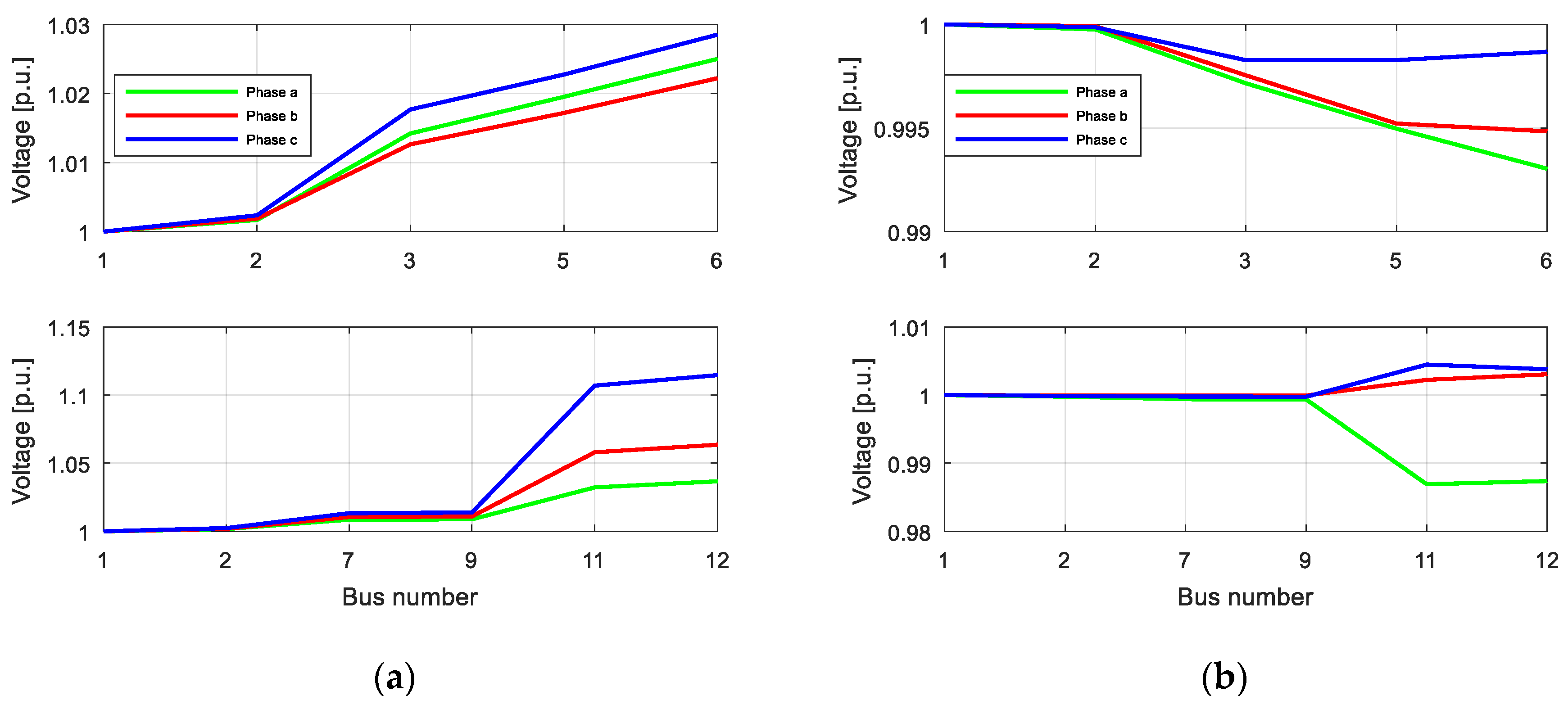
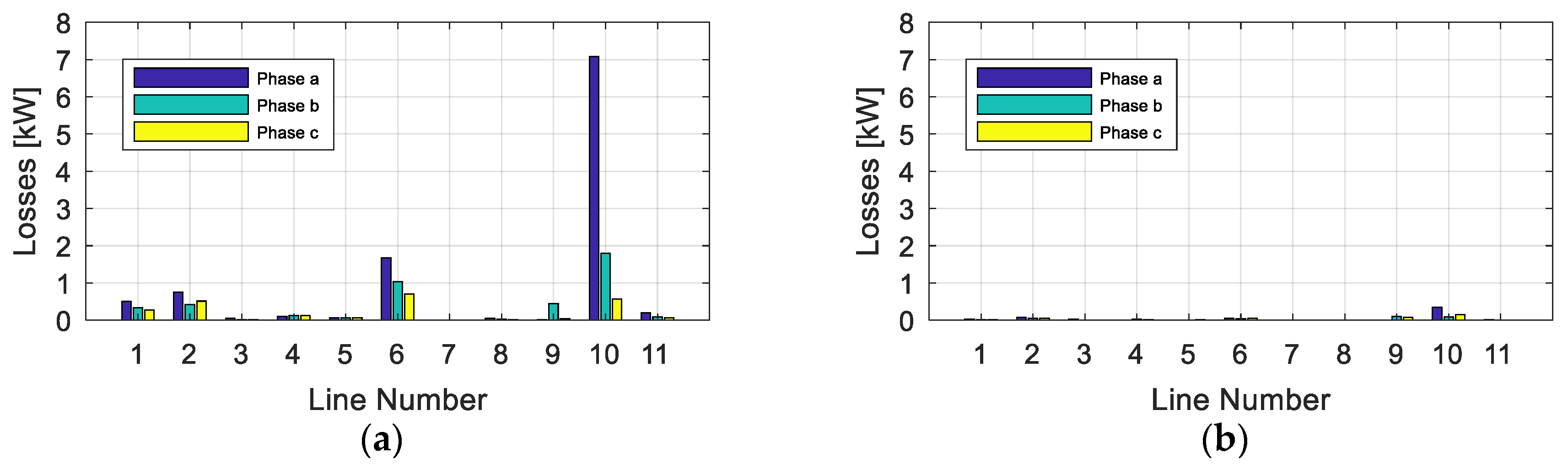
4.4. Scenario 1: PV Production, No Imbalance Compensation and No Reactive Power Compensation

This scenario represents a common situation in a network where there is a high number of consumers injecting active power when there is an excess of production in relation to consumption. The power injection is done in an equal way, that is, the inverter equitably distributes the power to be injected into the phases.
As can be seen in Figure 9a, since production is greater than consumption, voltages generally increase at the buses that are furthest from the MV/LV transformation. It is also possible to verify that the power injection does not improve the phase balance. The day of highest radiation is the worst case, with an overvoltage exceeding 0.1 p.u in bus 12 in phase c. On the other hand, on the day of the lowest radiation, the voltage levels improve, approaching 1 p.u. This happens because the power generated almost equals the power consumption (see Figure 6b as an example of a prosumer).
As in the day of highest radiation the power generated by the PV systems is much higher than the consumption, the power flow increased, and consequently the losses (Figure 10a) significantly increased. On the other hand, on the day with the lowest radiation, the losses decreased reaching very low values (Figure 10b). As mentioned, this is due to the fact that the produced power is close to the consumed power, thus reducing the power flow in the network.

4.5. Scenario 2: PV Production, Imbalance Compensation and No Reactive Power Compensation

With respect to scenario 1 (Figure 9), it is possible to observe in Figure 11 that voltage imbalance is reduced on both days and that phase voltages are nearly equal. It is also possible to verify a reduction of the over-voltages, namely, from 0.11 p.u to 0.07 p.u., in the phase c of bus 12, for the day with the highest radiation.
Analyzing Figure 12 and comparing it with the results obtained for the previous scenario (Figure 10), it can be seen that, in general, the phase balance led to a reduction in losses, although there have been small increases in certain phases. This is due to the increase in power injection in those phases in order to compensate for the imbalance.

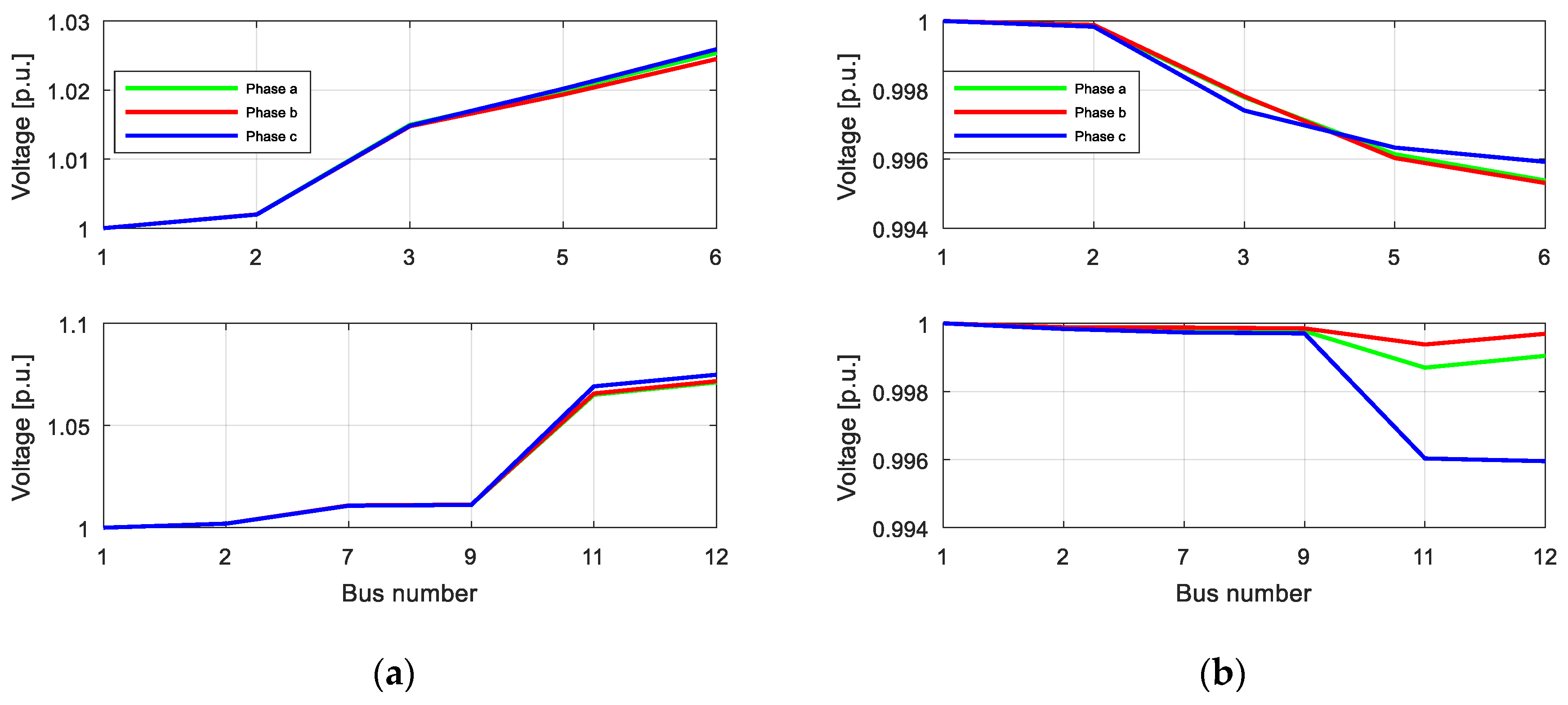
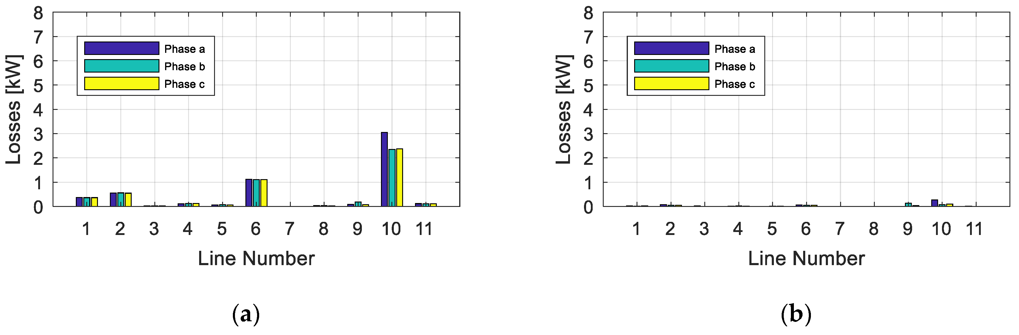
4.6. Scenario 3: PV Production, Imbalance and Reactive Power Compensation

Comparing Figure 13 with the respective profiles for Scenario 2 (Figure 11), it is observed that they are very similar, so it can be confirmed that the reactive power compensation has little impact on the voltage profiles (this is due to the high R/X ratio, a typical situation in LV networks). However, Figure 14 shows that the reactive power compensation led to a reduction in line losses.

4.7. Comparative Analysis

In order to evaluate the impact on the LV network of the different approaches, Table 2 shows, for the days of highest and lowest total radiation, the total active power losses ( P l o s s ) and the active power delivered from the MV/LV transformer, at bus 1 ( P i n j , 1 ). This last value was obtained from the difference between the total power consumption (loads and losses) and the total PV power generation.
From the results obtained, it is possible to verify that, on the day of highest radiation, when there are no auxiliary services (Scenario 1), the injection of the PV generated power leads to a large increase (about 100%) in losses with respect to the baseline scenario. However, the auxiliary services provided by the PV inverters allows the reduction of the total network losses. In fact, compared to Scenario 1, total losses decrease about 11.6% in Scenario 2 and 15.5% in Scenario 3.
On the other hand, on the day of lowest radiation, and for the case where there is no PV production, the losses are higher comparing to the day of highest radiation, since the consumption is higher. With the injection of the power produced by the PV systems in the network, the losses decrease about 88%. When ancillary services are considered, and compared to Scenario 1, losses decrease about 12.9% in Scenario 2 and 66.5% in Scenario 3.
Finally, it should be noted that the negative values of the bus 1 injected power means that power is being supplied to the MV distribution network, due to the fact that production is higher than consumption. Although this implies more available power, those networks were not designed to have reverse power flows, what could cause problems in the protection systems, which must be evaluated [36,37].

5. Conclusions

This work address the use and management of ancillary services provided by PV systems in a three-phase, unbalanced LV network. These networks are generally affected by several factors such as imbalances and voltage profiles that do not comply with legislation. Taking into account the high increase of the PV systems in this type of networks, it has been verified that these problems have tendency to worsen. In fact, contrary to what happened till now, in this new context, it appears overvoltages, especially in summer, when there is more solar radiation.
To deal with these problems, that have been little addressed so far, novel improved control strategies for the electronic converters have been proposed. Thus, the strategies try to compensate the load imbalances, to alleviate the overvoltages caused by the injection of active power from the PV panels and to minimize the reactive power flow in the network.
It has been presented a case study of a LV network with 240 consumers (105 single-phase and 135 three-phase) distributed in twelve buses. Through the obtained results, it is verified that, by injecting active and reactive power into the network in a proper way, it is possible to compensate the load imbalance, improving the voltage profiles and reducing line losses.
The results have shown that the proposed control strategy for the PV inverters is feasible, can be implemented locally and allows to improve the voltage regulation in four-wire LV distribution networks with high penetration rates of PV production systems in self-consumption regime. The practical application of the proposed strategy will allow to increase the supply capacity of these networks while increasing their capacity to integrate a greater production of renewable energy.
The development of this work has led to some new research questions. The following represent some topics which the authors continue working in: (i) include simulation cases considering energy storage systems (battery chargers for electric vehicles); (ii) include load matching; (iii) simulate using real data obtained from smart meters and validate results from real measurements; (iv) use alternative algorithms, such as genetic algorithms.

Author Contributions

Conceptualization, F.B.-G., V.F.P. and J.L.S.; Funding acquisition, F.B.G., E.G.R. and J.F.M.; Investigation, F.B.G., V.F.P. and J.F.M.; Methodology, M.I.M.-M., E.G.-R.; Software, V.F.P. and J.L.S.; Supervision, E.G.-R., M.I.M.-M., E.R.-C. and J.F.M.; Validation, E.G.-R. and E.R.-C.; Writing – original draft, F.B.-G.; Writing—review & editing, M.I.M.-M., E.G.-R., J.F.M. and E.R.-C.

Funding

This work was supported by Junta de Extremadura (Regional Government), Spain, under the Mobility Scholarship Program for Teaching and Research Staff of the Autonomous Community of Extremadura 2018.; by the Spanish Agencia Estatal de Investigación (AEI) and Fondo Europeo de Desarrollo Regional (FEDER), under Project TEC2016-77632-C3-1-R (AEI/FEDER, UE); and through FCT under contracts UID/CEC/50021/2019, Pest-E/EEI/LA0021/2014 and UID/Multi/00308/2019.

Conflicts of Interest

The authors declare no conflict of interest.

References

  1. Bellekom, S.; Arentsen, M.J.; van Gorkum, K. Prosumption and the distribution and supply of electricity. Energy Sustain. Soc. 2016, 6, 1–17. [Google Scholar] [CrossRef]
  2. Postigo Marcos, F.; Mateo Domingo, C.; Gómez San Román, T.; Palmintier, B.; Hodge, B.; Krishnan, V.; de Cuadra García, F.; Mather, B. A Review of Power Distribution Test Feeders in the United States and the Need for Synthetic Representative Networks. Energies 2017, 10, 1896. [Google Scholar] [CrossRef]
  3. Schneider, K.P.; Mather, B.A.; Pal, B.C.; Ten, C.W.; Shirek, G.J.; Zhu, H.; Fuller, J.C.; Pereira, J.L.R.; Ochoa, L.F.; de Araujo, L.R.; et al. Analytic Considerations and Design Basis for the IEEE Distribution Test Feeders. IEEE Trans. Power Syst. 2018, 33, 3181–3188. [Google Scholar] [CrossRef]
  4. Mateo, C.; Prettico, G.; Gómez, T.; Cossent, R.; Gangale, F.; Frías, P.; Fulli, G. European representative electricity distribution networks. Int. J. Electr. Power Energy Syst. 2018, 99, 273–280. [Google Scholar] [CrossRef]
  5. Teodorescu, R.; Liserre, M.; Rodríguez, P. Grid Converters for Photovoltaic and Wind Power Systems, 1st ed.; Wiley: Chichester, UK, 2011. [Google Scholar]
  6. Matos, D.; Catalão, J.P.S. Geração Distribuída e os seus Impactes no Funcionamento da Rede Elétrica: Parte 1. In Proceedings of the International Conference on Engineering, Covilhã, Portugal, 27–29 November 2013. [Google Scholar]
  7. Röhrig, C.; Rudion, K.; Styczynski, Z.A.; Nehrkorn, H.J. Fulfilling the standard EN 50160 in distribution networks with a high penetration of renewable energy system. In Proceedings of the 2012 3rd IEEE PES Innovative Smart Grid Technologies Europe (ISGT Europe), Berlin, Germany, 14–17 October 2012. [Google Scholar]
  8. Masoum, A.S.; Moses, P.S.; Masoum, M.A.S.; Abu-Siada, A. Impact of rooftop PV generation on distribution transformer and voltage profile of residential and commercial networks. In Proceedings of the 2012 IEEE PES Innovative Smart Grid Technologies (ISGT), Washington, DC, USA, 16–20 January 2012. [Google Scholar]
  9. Rodriguez-Calvo, A.; Cossent, R.; Frías, P. Integration of PV and EVs in unbalanced residential LV networks and implications for the smart grid and advanced metering infrastructure deployment. Int. J. Electr. Power Energy Syst. 2017, 91, 121–134. [Google Scholar] [CrossRef]
  10. CENELEC. Voltage Characteristics of Electricity Supplied by Public Distribution Systems; European Standard EN50160; CENELEC: Brussels, Belgium, 2015. [Google Scholar]
  11. Yu, H.; Pan, J.; Xiang, A. A multi-function grid-connected PV system with reactive power compensation for the grid. Sol. Energy 2005, 79, 101–106. [Google Scholar] [CrossRef]
  12. Piegari, L.; Tricoli, P. A control algorithm of power converters in smart-grids for providing uninterruptible ancillary services. In Proceedings of the 14th International Conference on Harmonics and Quality of Power—ICHQP 2010, Bergamo, Italy, 26–29 September 2010. [Google Scholar]
  13. Pires, V.F.; Martins, J.F.; Silva, J.F. A control structure for a photovoltaic supply system with power compensation characteristics suitable for smart grid topologies. In Proceedings of the 2013 International Conference-Workshop Compatibility and Power Electronics, Ljubljana, Slovenia, 5–7 June 2013. [Google Scholar]
  14. Fernao Pires, V.; Husev, O.; Vinnikov, D.; Martins, J.F. A control strategy for a grid-connected PV system with unbalanced loads compensation. In Proceedings of the 2015 9th International Conference on Compatibility and Power Electronics (CPE), Costa da Caparica, Portugal, 24–26 June 2015. [Google Scholar]
  15. Kim, E.; Kim, G.; Hwang, C.; Jeon, J.; Ahn, J. A novel three-phase four-leg inverter based load unbalance compensator for stand-alone microgrid. Int. J. Electr. Power Energy Syst. 2015, 65, 70–75. [Google Scholar] [CrossRef] [Green Version]
  16. Shahnia, F.; Wolfs, P.J.; Ghosh, A. Voltage Unbalance Reduction in Low Voltage Feeders by Dynamic Switching of Residential Customers Among Three Phases. IEEE Trans. Smart Grid 2014, 5, 1318–1327. [Google Scholar] [CrossRef] [Green Version]
  17. Su, X.; Masoum, M.A.S.; Wolfs, P.J. Optimal PV Inverter Reactive Power Control and Real Power Curtailment to Improve Performance of Unbalanced Four-Wire LV Distribution Networks. IEEE Trans. Sustain. Energy 2014, 5, 967–977. [Google Scholar] [CrossRef]
  18. Gagrica, O.; Nguyen, P.H.; Kling, W.L.; Uhl, T. Microinverter Curtailment Strategy for Increasing Photovoltaic Penetration in Low-Voltage Networks. IEEE Trans. Sustain. Energy 2015, 6, 369–379. [Google Scholar] [CrossRef]
  19. Su, X.; Masoum, M.A.S.; Wolfs, P.J. Multi-Objective Hierarchical Control of Unbalanced Distribution Networks to Accommodate More Renewable Connections in the Smart Grid Era. IEEE Trans. Power Syst. 2016, 31, 3924–3936. [Google Scholar] [CrossRef]
  20. Jin, P.; Li, Y.; Li, G.; Chen, Z.; Zhai, X. Optimized hierarchical power oscillations control for distributed generation under unbalanced conditions. Appl. Energy 2017, 194, 343–352. [Google Scholar] [CrossRef]
  21. Alam, M.J.E.; Muttaqi, K.M.; Sutanto, D. Community Energy Storage for Neutral Voltage Rise Mitigation in Four-Wire Multigrounded LV Feeders with Unbalanced Solar PV Allocation. IEEE Trans. Smart Grid 2015, 6, 2845–2855. [Google Scholar] [CrossRef]
  22. Brandao, D.I.; de Araújo, L.S.; Caldognetto, T.; Pomilio, J.A. Coordinated control of three- and single-phase inverters coexisting in low-voltage microgrids. Appl. Energy 2018, 228, 2050–2060. [Google Scholar] [CrossRef]
  23. Unigwe, O.; Okekunle, D.; Kiprakis, A. Economical distributed voltage control in low-voltage grids with high penetration of photovoltaic. CIRED Open Access Proc. J. 2017, 2017, 1722–1725. [Google Scholar] [CrossRef]
  24. Olivier, F.; Aristidou, P.; Ernst, D.; Van Cutsem, T. Active Management of Low-Voltage Networks for Mitigating Overvoltages Due to Photovoltaic Units. IEEE Trans. Smart Grid 2016, 7, 926–936. [Google Scholar] [CrossRef]
  25. Fang, Y.; Li, R.; Wang, L.; Song, B.; Li, E.; Zhang, Q. Research of active load regulation method for distribution network considering distributed photovoltaic and electric vehicles. J. Eng. 2017, 2017, 2444–2448. [Google Scholar] [CrossRef]
  26. Exposto, B.; Monteiro, V.; Pinto, J.G.; Pedrosa, D.; Meléndez, A.A.N.; Afonso, J.L. Three-phase current-source shunt active power filter with solar photovoltaic grid interface. In Proceedings of the 2015 IEEE International Conference on Industrial Technology (ICIT), Seville, Spain, 17–19 March 2015. [Google Scholar]
  27. Dai, X.; Chao, Q. The research of photovoltaic grid-connected inverter based on adaptive current hysteresis band control scheme. In Proceedings of the 2009 International Conference on Sustainable Power Generation and Supply, Nanjing, China, 6–7 April 2009. [Google Scholar]
  28. Blorfan, A.; Wira, P.; Flieller, D.; Sturtzer, G.; Mercklé, J. A three-phase hybrid active power filter with photovoltaic generation and hysteresis current control. In Proceedings of the IECON 2011—37th Annual Conference of the IEEE Industrial Electronics Society, Melbourne, Australia, 7–10 November 2011. [Google Scholar]
  29. Feng, W.; Sun, K.; Guan, Y.; Guerrero, J.M.; Xiao, X. Active Power Quality Improvement Strategy for Grid-Connected Microgrid Based on Hierarchical Control. IEEE Trans. Smart Grid 2018, 9, 3486–3495. [Google Scholar] [CrossRef] [Green Version]
  30. Milanes-Montero, M.I.; Barrero-Gonzalez, F.; Pando-Acedo, J.; Gonzalez-Romera, E.; Romero-Cadaval, E.; Moreno-Munoz, A. Active, reactive and harmonic control for distributed energy micro-storage systems in smart communitie homes. Energies 2017, 10, 448. [Google Scholar] [CrossRef]
  31. Milanes-Montero, M.I.; Barrero-Gonzalez, F.; Pando-Acedo, J.; Gonzalez-Romera, E.; Romero-Cadaval, E.; Moreno-Munoz, A. Smart Community Electric Energy Micro-Storage Systems with Active Functions. IEEE Trans. Ind. Appl. 2018, 54, 1975–1982. [Google Scholar] [CrossRef]
  32. Fernão Pires, V.; Romero-Cadaval, E.; Vinnikov, D.; Roasto, I.; Martins, J.F. Power converter interfaces for electrochemical energy storage systems—A review. Energy Convers. Manag. 2014, 86, 453–475. [Google Scholar] [CrossRef]
  33. Camilo, F.M.; Castro, R.; Almeida, M.E.; Pires, V.F. Self-consumption and storage as a way to facilitate the integration of renewable energy in low voltage distribution networks. IET Gener. Transm. Distrib. 2016, 10, 1741–1748. [Google Scholar] [CrossRef]
  34. Caracterização da procura de energia elétrica em 2018. Entidade Reguladora dos Serviços Energéticos de Portugal. Available online: www.erse.pt (accessed on 30 September 2018).
  35. PVGIS. Photovoltaic Geographical Information System—Interactive Maps. Available online: http://re.jrc.ec.europa.eu/pvgis/apps4/pvest.php# (accessed on 30 September 2018).
  36. Liu, X.; Shahidehpour, M.; Li, Z.; Liu, X.; Cao, Y.; Tian, W. Protection Scheme for Loop-Based Microgrids. IEEE Trans. Smart Grid 2017, 8, 1340–1349. [Google Scholar] [CrossRef]
  37. Tekpeti, B.S.; Kang, X.; Huang, X. Fault analysis of solar photovoltaic penetrated distribution systems including overcurrent relays in presence of fluctuations. Int. J. Electr. Power Energy Syst. 2018, 100, 517–530. [Google Scholar] [CrossRef]
Figure 1. PV system with four-leg power inverter.
Energies 12 00972 g001
Figure 2. Direction convention for power flows at a generic bus j.
Energies 12 00972 g002
Figure 3. Flowchart for the phase imbalance compensation algorithm.
Energies 12 00972 g003
Figure 4. Flowchart for the reactive power compensation algorithm.
Energies 12 00972 g004
Figure 5. LV test network.
Energies 12 00972 g005
Figure 6. Load profile and PV generation for a prosumer example, for the days along a year with: (a) highest total radiation and (b) lowest total radiation.
Energies 12 00972 g006
Figure 7. Scenario 0. Bus voltage profiles for branches B1 (up) and B2 (down) at the hours: (a) Peak-H and (b) Peak-L.
Energies 12 00972 g007
Figure 8. Scenario 0: Line losses at the hours: (a) Peak-H and (b) Peak-L.
Energies 12 00972 g008
Figure 9. Scenario 1: Bus voltage profiles for branches B1 (up) and B2 (down) at the hours: (a) Peak-H and (b) Peak-L.
Energies 12 00972 g009
Figure 10. Scenario 1: Line losses at the hours: (a) Peak-H and (b) Peak-L.
Energies 12 00972 g010
Figure 11. Scenario 2: Bus voltage profiles for branches B1 (up) and B2 (down) at the hours: (a) Peak-H and (b) Peak-L.
Energies 12 00972 g011
Figure 12. Scenario 2: Line losses at the hours: (a) Peak-H and (b) Peak-L.
Energies 12 00972 g012
Figure 13. Scenario 3: Bus voltage profiles for branches B1 (up) and B2 (down) at the hours: (a) Peak-H and (b) Peak-L.
Energies 12 00972 g013
Figure 14. Scenario 3: Line losses at the hours: (a) Peak-H and (b) Peak-L.
Energies 12 00972 g014
Table 1. Line impedances for the LV test network.
LineL1L2L3L4L5L6L7L8L9L10L11
R (Ω)0.000740.019740.025470.015890.030560.004460.002130.000430.057950.075130.01891
X (Ω)0.000330.006300.008130.007960.009750.001420.001070.000210.017800.023970.00581
Table 2. Total power and energy losses and power injected from bus 1.
Scenario NumberHighest Radiation DayLowest Radiation Day
P l o s s (kW) P i n j , 1 (kW) P l o s s (kW) P i n j , 1 (kW)
Scenario 0 (Baseline)8.50138304.2036510.96334353.68494
Scenario 117.23334−471.073051.24492−15.10588
Scenario 215.23509−473.07131.08481−15.26599
Scenario 314.56905−473.737340.41763−15.93317

