1. Introduction
After being produced in power plants, the electrical energy is delivered to the consumers through the existing lines. These lines include the high-voltage transmission lines, the sub-transmission lines (medium voltage), and the distribution lines (primary and secondary). One of the important issues that must be dealt with in the distribution systems is the problem of fault occurrences in these networks’ lines, which is inevitable. Fault location plays a key role in fault management in such systems. Fault location in the distribution systems, however, is a challenging task. This is because of the condition and complex topology of distribution networks. In distribution networks, there are sections with the same distance from the beginning of the feeder; important loads are present; and lines are usually hybrid including cable, aerial, and ground. These specific features, along with the clear dependency of societies and the sustainable development on the security of supply and the fact that faults in the distribution networks, are the main reasons for power supply disruption, as well as for wide investments in automatic fault location methods in distribution networks. Fault location can eliminate and shorten unwanted interruptions and can reduce the costs of power restoration.
Usually, in distribution systems, the fault location methods are expressed based on the manual benchmarking of power cuts using the consumers’ contacts, primary voltage, and electrical network parameters, as well as the components of current and voltage in distribution networks. However, recently, methods have been presented that have used advanced measurement systems.
Many fault location methods have been developed in the literature. To investigate these techniques and understand different features, one needs to pay special attention to the following:
Type of considered line model
Type of considered load model
Considering the constant load power model or presenting load estimation
Heterogeneity and unbalance
Examining the types of fault
Estimating the fault section
How to use the type of voltage signal and used current (instantaneous values, phasor, and symmetrical components)
In what follows, several methods are investigated. The method proposed in the work of [
1], firstly divides the distribution network into several areas and then, for each area, a set of breakers and related protection systems are included. Then, it assumes that when a fault occurs in the system, all information of the protection equipment is activated, and the status of breakers is available in the control center. Within this method, a databank that represents the connection of operating equipment and faulty areas is developed and the neural network is trained. Then, when a fault occurs in each area, the neural network specifies the fault area based on the information of the breakers’ status and the protective equipment and existing databanks. The disadvantage of this method is that it considers breakers and protective equipment separately for each area, which is not practically possible. Databanks in these methods rely on information of protection devices and whenever a change occurs in the network, information should be updated and recorded. This reduces the efficiency and accuracy for the real networks. In the work of [
2], a method like the previous one is given for locating the fault in distribution networks. The difference is that in this method, load estimation and line model parameters have been used to enhance the accuracy of the given method [
3]. There are two advantages for the proposed method compared with the one presented in the work of [
3], namely, independency from fault resistance and increased accuracy. These advantages make the proposed method superior over methods presented in the work of [
3]. The authors of [
4] discuss the importance of quick fault location in electrical distribution lines, thus continuing the services and improving the reliability indicators of the system, and then they present a method based on current patterns and time pattern of currents at the beginning of feeders so that the faulty section is specified. Upon the placement of the protective equipment of distribution networks and their special coordination, they act in a way that they create a unique time–current pattern for a fault in each section. It should be mentioned that this method improves the performance of impedance methods, and its difference with the method proposed in this paper is in the accuracy of the methods. The proposed method obtains higher performance and accuracy compared with the similar methods, while trying to locate faulty sections. In another paper [
5], the method deals with observing the electric power quality in feeder distribution through presenting a current waveform-based model, and then uses it for locating the fault in such a way that it takes advantage of current information of the feeder model to estimate the fault currents and compare it with data obtained from the power quality. In other works [
6,
7], by combining impedance and frequency area methods and using the information of both areas, new methods are given that improve the accuracy and performance of these methods compared with the previously examined methods. These methods determine probable fault locations using impedance patterns and then specify the exact fault section through frequency analysis. One of the disadvantages of these methods is their incompatibility with the continuous changes in the distribution network due to wide extension and numerous changes.
In the work of [
8], a fault location method based on smart feeder-meters with the capability of supervising the voltage drop has been proposed. The main idea of the work is to explore and measure the voltage by monitoring different buses in distribution systems to estimate the exact fault location. The values estimated through the relationship between voltage deviations obtained from each feeder-meter and the measured fault current, which has been calculated based on the bus impedance matrix, are shown in view of fault presence in different points. To improve the accuracy and precision of this method, loads are shown by constant impedance models and then they are attributed to the bus impedance matrix. With regards to the current structure of the electrical distribution networks, applying this method is too costly. In addition, in these methods, it is not required to use new equipment; therefore, they do not require huge investment in new devices and equipment, which facilitates the wide adoption of the methods. Using new equipment not only imposes high costs, but also requires new and possibly complicated design processes for deployment. In the work of [
9], probable fault locations in a highly noisy environment are determined with the help of impedance methods. Then, a smart method is presented that determines the fault section based on properties extracted from the voltage at the beginning of feeders and introduces a point as the main fault location from among the probable locations. However, there are problems in its databank that need to be addressed. Another point that should be mentioned is the shortcomings of the used algorithm. The algorithm needs a good kernel function and an accurate parameter selection, which affects the accuracy. It should be noted that the proposed method does not have any of the mentioned shortcomings. In another paper [
10], an active and hierarchical location method is given for the ring distribution networks in neural and ineffective points for single-phase faults to earth. Within this method, by single-phase faults to earth in two distribution networks, a neural closed loop with single-phase faults to earth is performed in two different topologies. Then, based on continuous changes in the closed loop currents, the fault section is specified. Finally, the exact position of single-phase faults to earth is determined by the help of technology of discrete wavelet transformation and support vector machine. As the types of fault are not considered, this method is not a complete and powerful one. In reference [
11] a method was presented for fault location in radial distribution systems in presence of distributed generation units. It locates fault based on voltage and current samples of feeder. In the impedance based method all sections of distribution systems are investigated to find fault location, first, based on voltage and current information before fault occurrence. Then, all sections are examined based on information registered in the location of main supply after fault occurrence. In reference [
12], an impedance method is presented to locate faults in an electric distribution network in which average line model is used to model the network; in the proposed method, results are good but the proposed method cannot detect exact fault location among multiple locations, thus it only determines fault distance. But on the Smart networks have the ability to record different parameters like voltage amplitude and phase, current and frequency in a specific period. Updating old networks using such a system is costly [
13]. In some method, smart measurements used in low voltage networks are considered. Information exchange under such condition requires complicated communication systems. Simultaneous detection of fault section considering specific topology of distribution networks is very important. In the following, algorithms proposed in [
14] and [
15] which require monitoring so that network operator can monitor and analyze and determine fault location after applying operational condition using GIS. Parallel transmission lines in power networks are described using a significant increase in mutual coupling. This results in occurrence of significant errors in impedance-based protection devices. Due to mutual coupling, total line impedance might change significantly as a result of common reflection impedances of other phases. Therefore, real line parameters deviate from parameters adjusted for relay. Significant errors are expected for parallel lines while locating fault. As reported in precious studies, various fault location algorithms have been proposed for distribution networks using one-sided measurements (at the beginning of the feeder) or double-sided measurements. However, mentioned algorithms consider a perfect realization of line parameters [
16]. The smart networks can record different parameters like the voltage amplitude and the phase current and frequency in a specific period [
17]. Updating old networks using such a system is costly. Another point that should be mentioned is its dependency on the mentioned devices; that is, this method should use smart feeder-meters to locate faults. This method is only effective for smart systems. This means that it is not effective for a wide range of current networks. As most of the current networks are conventional networks, this is one of the most important shortcomings of such methods. Note that the proposed method can be used for any network type and it resolves these problems. In other works [
18,
19], smart measurements used in the low voltage networks are considered. Information exchange under such condition requires complicated communication systems. Simultaneous detection of fault section considering specific topology of distribution networks is very important, as mentioned in the investigation of the previous studies, they do not need too much investment. The new proposed method only uses the available information and does not require new investment in hardware.
The algorithms that have been proposed in the works of [
20,
21] require monitoring. The network operator can monitor, analyze, and determine fault location after applying operational condition using Geographic Information System (GIS). Parallel transmission lines in power networks are described using a significant increase in mutual coupling. In the occurrence of the significant faults in impedance-based protection devices, the previously mentioned problems can be observed. In one study, high-level monitoring is required. In another study, methods developed for transmission lines are used that do not match the nature of distribution networks of the main and side sections and branches that are comprised. These problems along with the scattering of distribution networks make using this method difficult and complicated. To address the shortcomings of these methods, new and simple methods for determining fault locations in distribution networks are needed. Because of the mutual coupling, the total line impedance might change significantly because of common reflection impedances of other phases. Therefore, real line parameters deviate from parameters adjusted for the relay. Significant errors are expected for parallel lines while locating faults. As reported in the previous studies, various fault location algorithms have been proposed for distribution networks using the one-sided measurements (at the beginning of the feeder) or double-sided measurements. However, the mentioned algorithms consider a perfect realization of line parameters [
22,
23,
24,
25]. The impact of such assumptions of the accuracy of the results cannot be ignored and the dependency on line parameters is high. This method requires an accurate measurement of the wave frequency and the velocity for determining fault locations. The resonance characteristics of the Direct Current (DC) capacitor at the fault location of the lines are exploited in the work of [
26], while there is dead-band in the system. In order to identify and replace faults in the modern distribution networks, multi-variety control methods are used, and the operational region is converted to a section that can be monitored. This is done to identify the main fault location, resolve the fault, and offer the alternative paths [
27]. Extracting specific components of the condition created during the fault and using a meta-heuristic algorithm are used in the work of [
28] and, finally, fault location is determined through marking. In other works [
29,
30,
31], pattern recognition has been used; that is, to achieve the goal, a series of laws and rules are considered, and finally a unique pattern is selected for fault detection in the power system. In these methods, each sample point in the power system signal is represented as (x
i, y
i), where y
i is the amplitude in volts or amperes of the ith point and x
i is the corresponding time and a set of features assigned to each initial pattern. The values of these features are calculated at the initial extraction step and used during the recognition process. These values help with recognizing patterns and measuring their parameters. That is, they are used quantitatively for qualitative and quantitative goals with an aim to implement protection relay to prevent damages caused by faults in power systems [
29,
30]. In the work of [
31], a hardware relay has been presented based on the pattern recognition methods, which detects faults in power system waveforms within a few microseconds after reading signal peaks. It should be mentioned that this method detects frequency and energy disorders, which provides a better performance and is more accurate compared with that presented in the work of [
30], considering the improvement in formulation and calculations. Indeed, it should be noted that data used in these references are offline and, considering high sampling frequency, large time-series cannot be generated from samples for transmission lines. In this reference, where sampling frequency is 800 Hz, 48,000 samples are generated per minute. As each peak is represented by a final symbol, an efficient analyzer should be implemented that can detect 6000 symbols per minute. Another point that should be considered in the works of [
29,
30,
31] is that these systems lack a primary waveform processing unit; finally, it should be said that despite the advantages of these methods, their performance in distribution networks has some problems, among which fundamental differences in distribution network lines including dispersion and side branches can be mentioned, which should be tested and evaluated. In the work of [
32], a method has been proposed that can detect illegal branches of the transmission line, and it does not require physical monitoring and allows the user to detect these faults remotely. This method is a subset of the mobile waves. This study [
32] has used line symmetry, the second echo, and power spectral density methods. This method employs power spectral density to find the illegal branches in MATLAB. Therefore, in lines without illegal branches, the power spectral density is focused on a specific frequency after pulse injection. A response to a pulse is another reflection pulse at the ending point, which includes a limited margin of the frequencies in discrete Fourier transform. However, if there are illegal branches in the line, reflection of the injected pulse adds more components to the frequency domain. Such methods can be used for the following problems: (a) detecting failures, the illegal side branches and the insulation losses in lines with a difficult access; (b) controlling power losses in the short transmission lines; (c) controlling the voltage drop or improving the characteristics of the lines; and (d) controlling the interferences or the changes in lines due to direct, illegal, or random operations. In another paper [
32], a method is developed for a transmission line. The transmission line condition is very different from distribution networks in that the performance of transmission line methods is not proper for distribution networks. In [
33], an impedance-based method is presented to locate faults in an electric distribution network in which an average line model is used to model the network. In this method, the results are good, but the method cannot detect the exact fault location among multiple locations, thus it only determines the fault distance. This has been shown in many studies [
34].
A detailed investigation and a state-of-art review confirm that it is necessary to develop new cost-effective and accurate methods specifically for distribution networks. This is because faults in the distribution grid are the main cause of disruption in the electricity supply. This is mostly because of the infrastructure aging and the extreme weather conditions. The current usual practice in fault and outage management is slow, expensive, and involves risks. The proposed method in this paper is not only simple and cost-effective, but also can be used under different conditions in different distribution networks, does not require specific tools and devices or installing specific facilities, and can locate faults with high accuracy. These features facilitate wide adoption of the proposed method.
The rest of this paper is organized as follows.
Section 2 describes a modified method for fault location and possible fault location based on an impedance method.
Section 3 presents the frequency analysis method for the generated transients to detect the faulty section. The results obtained from simulations in MATLAB considering an 11-node distribution feeder are given in
Section 4. To test the proposed approach, the power system simulator is also used in
Section 5. Finally, the conclusion and future works are presented in
Section 6.
2. The Modified Method for Fault Distance Determination
As the fault location methods in power distribution networks (PDNs) are divided into fault distance determination and fault section estimation, in this part, at first a modified impedance-based fault location method is presented. As it may determine some possible fault points, a new fault section estimation method is described that determines the real location of the fault among all the possible fault points. It is worth noting that the proposed algorithm for determining the section of the fault is independent to the algorithm used for determining the fault distance. These two algorithms are complementary for achieving the real location of the fault among the possible fault locations. Generally, other impedance-based fault location methods can be used for determining the possible locations of the fault. However, because of the high accuracy of the presented method in the work of [
3], this method is used for determining the possible fault location. In the following subsection, the principals of this method are described.
2.1. The Proposed Method for Fault Location
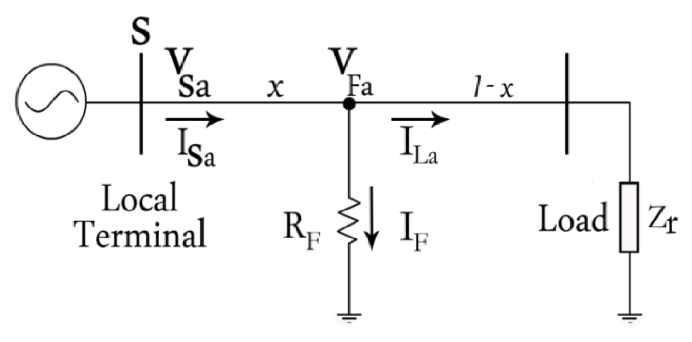
The fault location method that is used in this paper for distribution systems is from the family of the impedance methods. To calculate the fault distance, information like distribution system parameters and a combination of pre-fault, post-fault, and through-fault currents and voltages (measured at the beginning of feeder) are used. Pre-fault values are used to calculate the initial condition of the power system and through-fault values are used as known variables in equations where their unknowns are the distance from the fault location and the fault resistance. The proposed method uses the impedance analysis method to locate the fault. In the impedance analysis of this paper, fifth order equations are used to determine fault locations, which are given in details in the following section. On the basis of the calculated distance of the fault, the fault is located. The proposed scheme assumes that pre-fault and through-fault voltage and currents are stored by the relay at the beginning of the feeder and this information is used to estimate the equivalent load and load current. The equivalent load and load current can be used to calculate fault resistance and fault distance in each section. Consider the circuit represented in
Figure 1. All loads after fault location are represented by an equivalent load
Zr. The total current transmitted to these loads is
ILa, which is equal to the current passing from the short circuit. The voltage and current are measured at the beginning of the feeder and the following relationship is satisfied:
: Impedance matrix
Impedance between phase a and b
Impedance between phase a and cn
This equation is given for a three-phase line where currents of each phase are given as
Ia,
Ib, and
Ic. To calculate the voltage along the line, an equation that is the product of current and impedance is considered. To maintain simplicity, this equation is given for the purpose of illustration; otherwise, as shown in the following section, equations can be obtained for the distributed line model. Then, the current is multiplied by the impedance, which is shown as impedance per unit length multiplied by distance, to calculate voltage where its single line diagram is shown in
Figure 1. It should be noted that in
Figure 1, because it is used to represent phase
a,
Ia would be
shown in
Figure 1, which is mentioned to preserve formulation and integration of
Ia.
In this section, VSa is the voltage at the beginning of the faulty section; VFa is the voltage of the fault location, which is the product of fault resistance (RF) and fault current (IF); and, finally, Zr is the equivalent load at the end of the rest of the line.
If the fault occurs on phase
a (single-phase to ground fault), the voltage equation would be as follows:
In Equation (2),
If can be calculated using the relationship between the load current and line current:
Therefore, voltage equation includes two unknown variables: fault distance (
x) and fault resistance (
Rf), which can be written as follows by taking the real and the imaginary parts of voltage equation and removing (
x):
In addition, coefficients A and B in relationship (4) are as follows:
Finally, the fault resistance is obtained. Note that index (r, i) represents the real and imaginary parts.
The equations for other faults can be obtained using the same method.
Knowing the fault resistance, the fault can be located using the impedance method, which will be described in the remainder of this section. The method is described as an algorithm. Steps are conducted in order and, finally, the main goal, which is determining the fault distance, is achieved. The calculations and formulation are performed as illustrated in the following section.
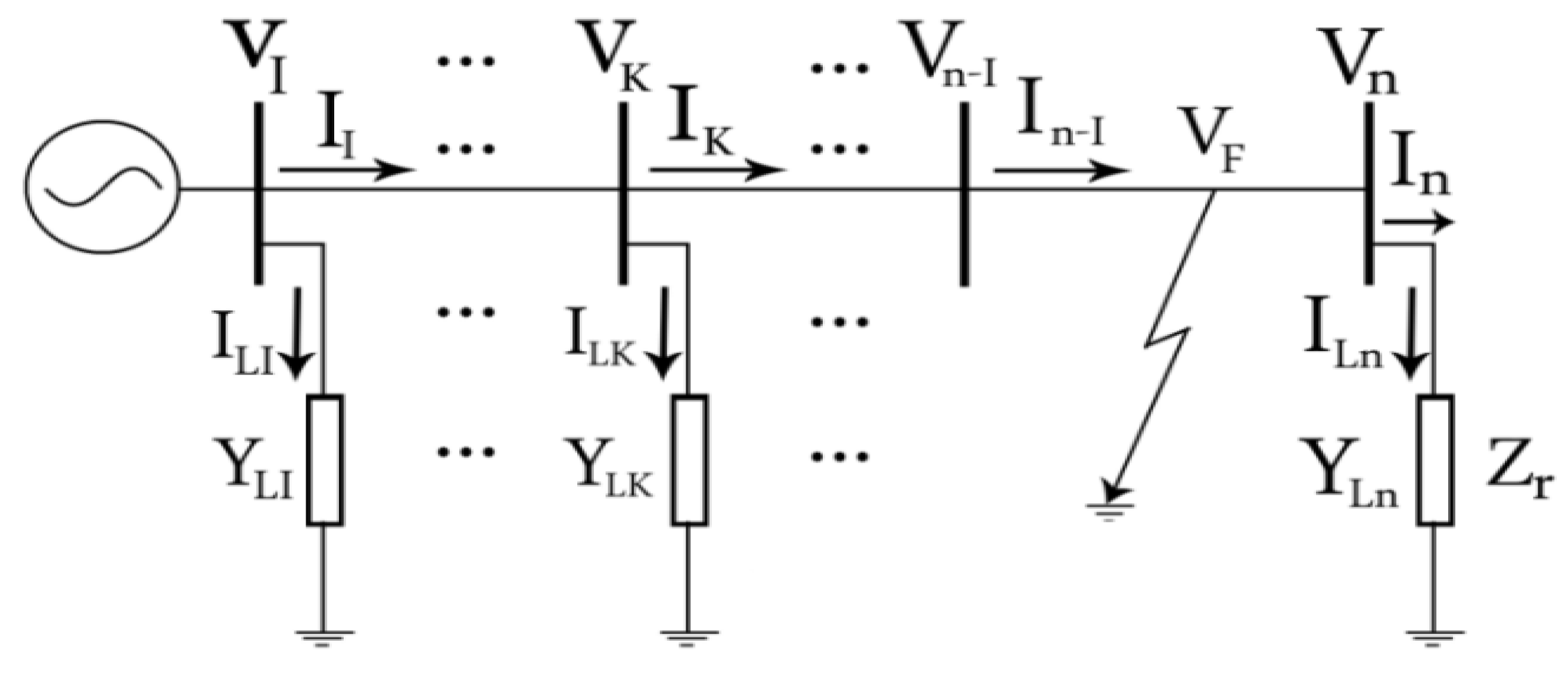
2.2. Determining Equivalent Load at the End of Each Section (DELS)
To describe the calculation of the equivalent load impedance at the end of each section, a sample network shown in
Figure 2 is considered. If the fault occurs on the line between node i and node j, the impedance of the equivalent load at the end of this section (equivalent impedance at ith bus) needs to be specified. This impedance is obtained using the following equation:
To determine each impedance
Z1,
Z2, and
Z3, the equivalent impedance seen from jth node in
Figure 2 and the equations given in the work of [
3] are used:
A single line diagram of a sample PDN is shown in
Figure 2. Suppose the section i–j is analyzed by the proposed method. The equivalent load impedance
is needed for analyzing the DELS in section i–j. In order to calculate it, the equivalent impedances of all paths that start from node j should be determined. It is calculated by (5). In this equation,
is determined from load flows. Each one of
Z1,
Z2, and
Z3 is determined by calculating the equivalent impedance seen from jth node. They are calculated by performing series and parallel of loads and line impedances. A distributed-parameter line model is assumed for each section, which is shown in
Figure 3. By this assumption, the equivalent impedance of each section, which is connected to node j and shown in
Figure 2, can be calculated by (6)–(8). Consequently,
,
and
. Matrix Z, which is the inverse of matrix Y, is an impedance matrix of the line and because Y is symmetric, Z is also symmetric about its main diagonal.
In order to show the above equations for modeling the circuit in DNs (considering the distributed line model), this problem is shown in the form of
Figure 3 which is in fact, the circuit model of each section of the sample DN.
2.3. Determining Current and Voltage at the Beginning of Each Section
Using the voltage and current information recorded at the beginning of the feeder, because each node is downstream of the node at the beginning of the feeder, the voltage of the downstream node
and input current of this node from the previous node (
) can be calculated using Equations (10) and (11):
where
is length of section
i–
j and coefficients
k0–
k5 are coefficients represented in calculations using the method presented in the work of [
3]. The associated formulation is given in
Appendix A (Equation (A1)).
To calculate the output current from node j to node 1 (
), the currents of different laterals and loads that are connected to node j are needed. Therefore,
is calculated by (
). In this equation,
is the sum of all currents that flow from all sections and loads connected to node j. This current can be calculated as follows:
: Output current from node j to node 1.
: sum of output currents from node j to the other branches except j − 1.
2.4. Location Algorithm of the Proposed Method in PDN
The fault location algorithm of the proposed method consists of nine steps, which are described in the following section.
Step 1. Fault type detection
In this step, the fault type is detected as single-phase to ground, two-phase to ground, two-phase to each other, and three-phase to ground.
Step 2. Determining the impedance of the equivalent load at the end of each section, and the current and voltage at the beginning of each section.
Step 3. Considering load current () to be the same before and after fault. In addition, assuming the output current from fault point towards end of section () to be equal to ().
Step 4. Assuming input current to the fault point from upstream (
) equal to output current from beginning node of the section (
). Note that the locations of different currents are shown in
Figure 4.
Step 5. Calculating the fault point using the following equation:
Step 6. Calculating the fault distance, that is, the value of x.
In this part, the location of the fault is determined using the presented impedance method in the work of [
11]. In this method, the distributed-parameter line model is used to improve the accuracy of the impedance-based fault location algorithm. On the basis of this model and depending on the fault type, two new equations are obtained, which can determine fault distance with high accuracy. To derive these equations, the voltage and current of fault point are calculated for each section at first, with respect to the voltage and current at the beginning of this section. As the distributed parameter line model is used, the function of hyperbolic cosine and sine with respect to fault distance exist in these equations. On the basis of Kirchhoff’s laws at the fault point, another equation can be written for fault point voltage with respect to fault current and fault resistance. If these two equations for voltage of fault point are set equal and considering the first three terms of Taylor expansion of hyperbolic cosine and sine function (
cosh(
γx) and
sinh(
γx)), a fifth order algebraic equation with respect to fault distance is obtained for each group of faults (grounded and ungrounded faults) [
3]. These equations are presented as follows:
Double phase fault (between phase
a and phase
b):
where
x is the fault distance from the beginning of feeder,
is the conjugate of fault current at phase
m, and the vectors
k0 to
k5 are defined in the
Appendix A (Equations (A1) and (A2)).
Where the final equations for calculating fault distance are simplified as follows:
Equation (13) can be used for different ground-connected faults and Equation (14) for different phase–phase faults.
Step 7. Checking if the algorithm is converged?
If yes, the algorithm is terminated and the value of x is printed; otherwise, go to Step 8.
Step 8. Determining the voltage of fault point again.
Fault in each section of the distribution system is estimated using convergence of this algorithm. In each step of the fault location using this algorithm,
VSa and
ISa are updated for the next step. This updating reduces faults caused by line losses and topology of PDN elements resulting from different loads along the lines. For better understanding,
Figure 5 is presented. Equations (15)–(17) are used for updating the voltage and current [
11].
Step 9. Updating
and
using Equations (18) and (19) and returning to
Step 3.
By updating the current and voltage, the algorithm is restarted and a new fault point is obtained, which is more accurate. This process is continued until the algorithm converges with the estimated fault point as an output. This algorithm is applied for each section of power distribution system (PDS). It is well known that the impedance-based fault location methods may estimate several locations of fault in different sections because its configuration has some laterals and sub laterals. These locations that are named the possible fault points have the same fundamental components of voltage and current at the beginning of feeder. Among them, distinguishing the actual location is very important. Thus, to determine the actual fault location, it is necessary to present an algorithm for fault section estimation. Up to this point, the proposed method determines possible fault points. To determine the real fault location, fault section should be determined. In the next section, a new method is proposed for fault section estimation.
3. Real Fault Location through Fault Section Estimation
Up to this point, possible fault locations are determined using the impedance method which was described in the last section. Now, the real fault location should be determined among all possible fault locations. To this end, the proposed method employs frequency component analysis of the real fault voltage and compares it with the simulated faults at possible locations.
The faulty section in the frequency domain is obtained based on comparing the absolute value of the theoretic natural frequencies, the natural frequency of the real fault voltage, and the simulated faults at possible locations. In the following section, this method is described. The real fault voltage and possible locations determined by the impedance method are used in the following three-step process to determine the real fault location.
Step 1. Fault is simulated at possible locations and the voltages at different locations are obtained:
V= fault voltage waveform at possible location 1
V= fault voltage waveform at possible location 2
•
•
•
V= fault voltage waveform at nth possible location
Step 2. In this step, the absolute value of frequency Fourier transform (FFT) of the fault voltage waveform is calculated for real fault and for fault at possible locations:
|FFT ()| = absolute value of FFT of real fault voltage
|FFT ()| = absolute value of FFT of fault voltage at possible location 1
|FFT ()| = absolute value of FFT of fault voltage at possible location 2
•
•
•
|FFT ()| = absolute value of FFT of fault voltage at the nth possible location
Step 3. In this step, a quantitative measure in terms of norm, that is,
is used for determining the main faulty section.
as follows:
After calculating for real fault voltage and all possible fault locations, the section that has the least is selected as the real faulty section.
In this method, a characteristic coefficient is calculated for each possible fault location (section estimated by the proposed method) using the fault voltage frequency component. For example,
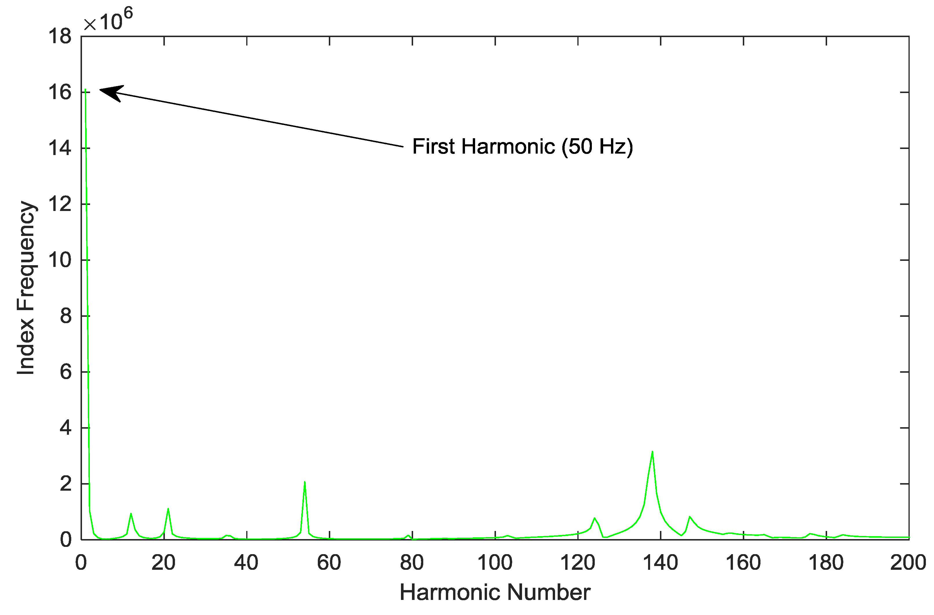
Figure 6 shows the voltage waveform of one of the phases (phase a) under steady state, before short circuit.
Figure 7 shows the voltage of this phase when a fault occurs. It should be mentioned that
Figure 6 and
Figure 7 represent one of the sections of the distribution feeder stored under normal and faulty conditions.
Considering
Figure 7, the transient generated in voltage waveform of phase “
a” can be seen. The characteristic coefficient of the real fault taken at the beginning of the feeder is calculated according to the following procedure. Then, the same fault is created in all possible locations using the proposed impedance method to extract the theoretic characteristic coefficient. These calculations begin from Equation (21).
Voltage stored at the beginning of the feeder is a sinusoidal voltage with respect to time, as shown in
Figure 7 and Equation (21).
In this step, the frequency component of the network voltage is determined using fast Fourier transform as follows:
In this step, the characteristic coefficient that is shown by α is defined. In fact, α is the characteristic coefficient of each branch that is extracted using voltage transient frequency component through-fault. This transient is caused by fault. The formula for this is given in the following:
where
α: characteristic coefficient of each branch
: frequency transform obtained from Fourier transform
: voltage of the phase in which fault has occurred (from relay at the beginning of the feeder)
t1: fault starting time (it can be seen clearly in
Figure 7)
t2: interruption time (in
Figure 7, it indicates storing time, 5 ms)
Considering Equation (23), the following parameters are defined:
: extracted characteristic coefficient of the real fault (using fault voltage stored in relay at the beginning of the feeder)
: extracted characteristic coefficient of estimated locations of feeder branches (using simulation and theoretic calculations)
In the description of Equation (23), its diagram is shown in
Figure 8. In the next step, it is necessary to determine the analysis index according to Equation (24) and one-to-one comparison in the frequency range using the obtained
and
.
where
: the analysis index of the proposed method for a distribution system with n branches
: the extracted characteristic coefficient of the real fault occurring in the sample system
: the extracted characteristic coefficient for all possible fault locations of the sample feeder branches (first to ith branch using simulation and theoretic calculations)
Analysis index: the proposed method calculates the index analysis through comparing the real fault characteristic coefficient and simulated faults for possible locations, which is represented as follows using the following symbol:
where
Finally, the proposed method introduces the branch that has the minimum analysis index as the section in which fault has occurred after calculating post-fault analysis indices and sorting these indices into descending order.
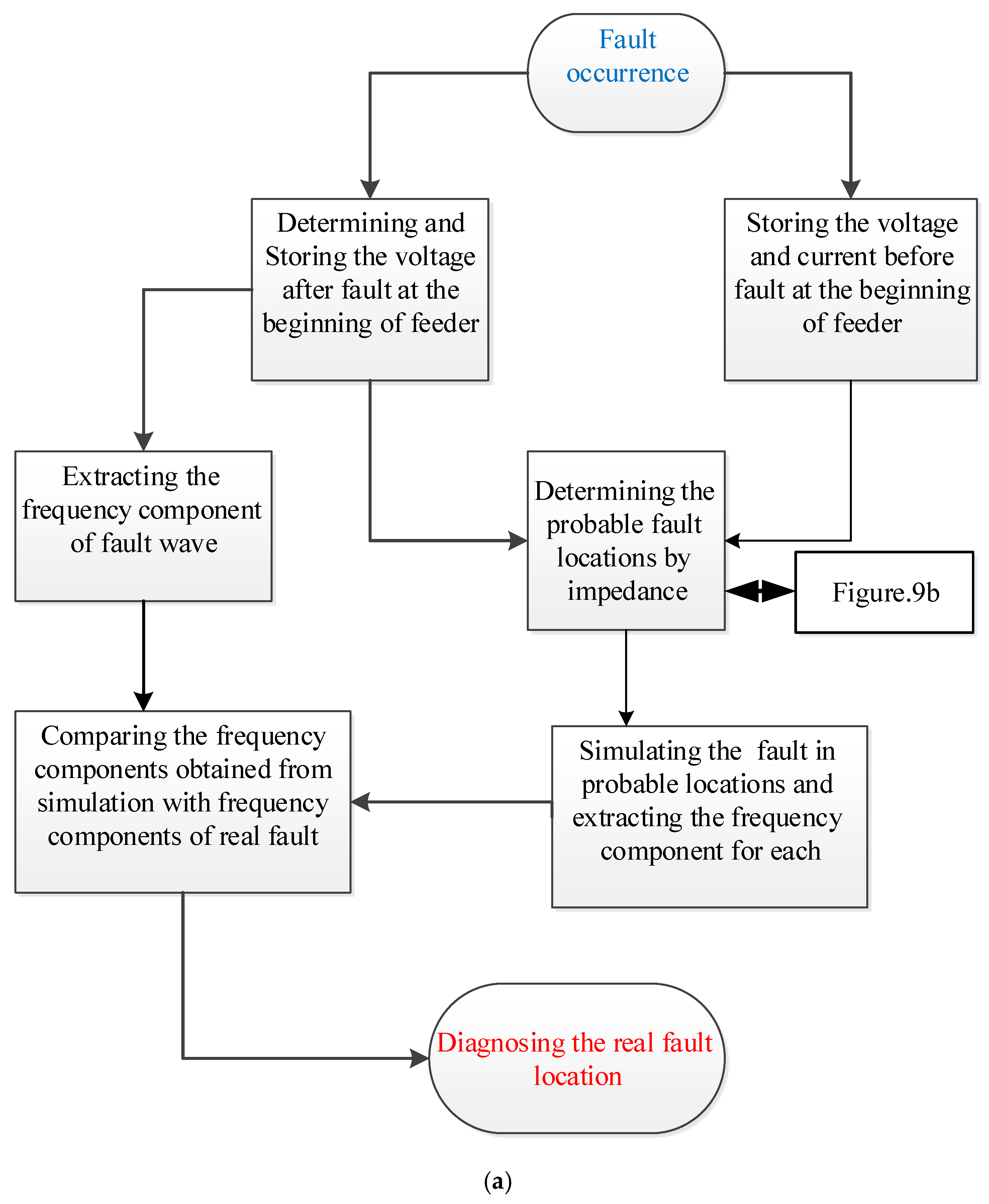
To give a better high-level overview of the method, a flowchart of the proposed method is shown in
Figure 9a, followed by
Figure 9b in which all steps of the proposed method are summarized.
Here, and after presenting the flowchart of the proposed method, complementary descriptions are given in brief. The proposed method, which employs information stored at the beginning of the feeder, starts its operation after operation of the relay when a fault occurs. In the first step and using voltage and current stored in the relay, fault is located according to the presented formulation; in fact, it should be said that to accomplish this goal, voltage and current relationships and the direct relationship between impedance and distance are used to determine fault distance. In the next step and considering the topology of distribution networks, the estimated distance can introduce one or several sections of the distribution network, where the complementary method determines accurate fault location based on the frequency component of each location and information of the main fault stored at the beginning of the relay; this is described in detail in the results analysis section, the explanations given here suffice for now in order to prevent duplicate discussions.
The simulation results on the test network are presented in the next section.
4. Sample Network, Analysis of the Results
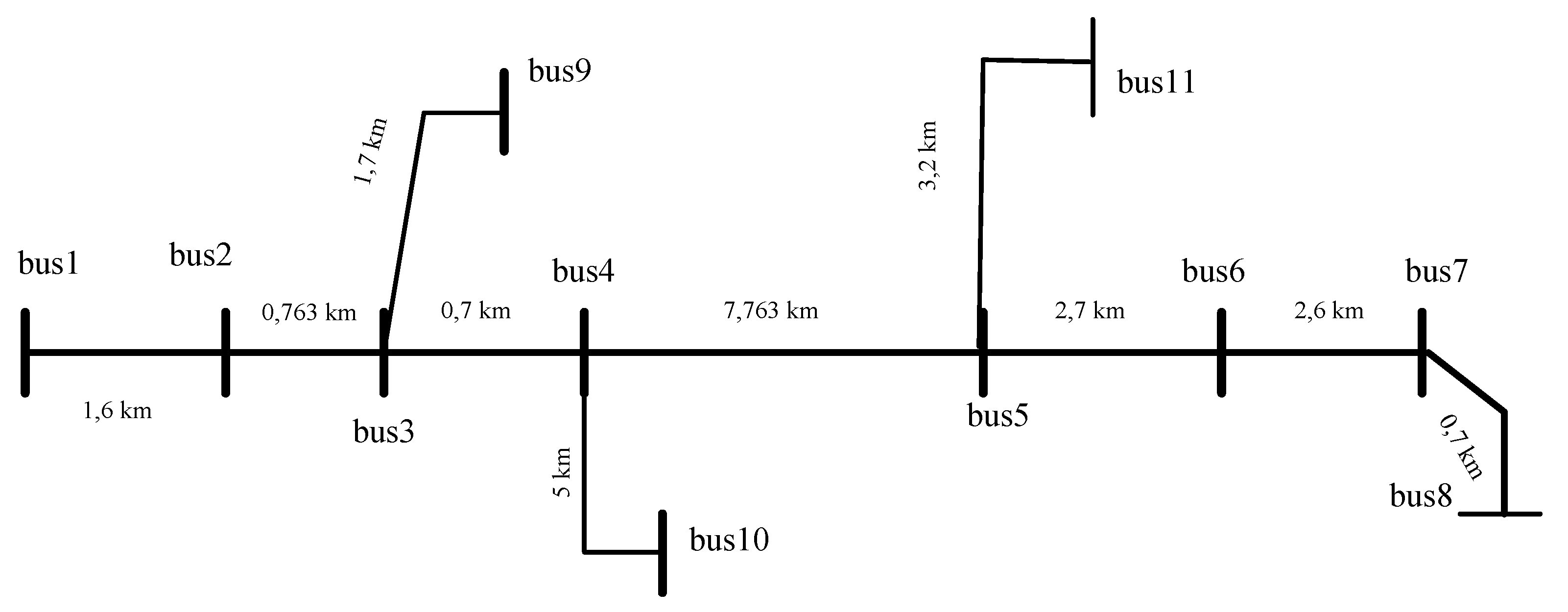
To evaluate the performance of the proposed scheme, a standard IEEE (The Institute of Electrical and Electronics Engineers) feeder with 11 nodes as shown in
Figure 10 is simulated in SIMULINK MATLAB (2016b, Natick, Massachusetts, MA, USA). The sample feeder with 11 nodes is a discrete line model. The feeder has some sections on the main body and sections with side branches of different lengths. The proposed fault location method is implemented in MATLAB. A single-line diagram of the feeder with main branch and side branches is shown in
Figure 10. Fault is simulated in all branches with different fault resistance and in different distances for the testing and evaluation of the proposed method. Fault resistance varies from small values to 150 ohms. In each simulation, the following conditions are created, and results are stored.
- (a)
Fault types
Ag, Bg, Cg, ABg, BCg, ACg, AB, BC, CA, and ABC
- (b)
Fault resistances: 0, 25, 50, 100, and 150 ohms.
- (c)
Fault distance: fault is created in different distances and different sections and the accuracy of the proposed method is evaluated.
It should be mentioned that for accurate simulation, lines are considered to be of the discrete model at a frequency of 50 Hz. The simulations are performed in SIMULINK and the sampling frequency is 256 samples per cycle.
In the simulations, the sample test network is an 11-node IEEE network simulated in MATLAB on a PC. First, the SIMULINK network is simulated in MATLAB, and then the information stored in workspace is used in an m-file. Finally, after running the final program, which is a MATLAB m-file, the main fault point is obtained.
4.1. Analysis of the Results
This section evaluates the accuracy and efficiency of the proposed method. The accuracy of the method is evaluated for different fault resistances, different fault locations, and different types of faults. An implementation of the proposed method and the obtained results confirms that the method has a satisfactory performance. Furthermore, the load changes and their impact on the accuracy of the proposed method are calculated through calculating the equivalent load (impedance load model is assumed to be constant) using pre-fault information when the system is stable.
In the following section, the accuracy of the proposed method in the fault location because of fault resistance and fault distance is shown for different types of faults.
In this step, the proposed method is tested on the test network. A fault is located in one section of the test network and it is run in MATLAB. Voltage and current information with the given sampling rate are given in the stored workspace. Fault creates a transient in voltage and current waveforms. The proposed impedance method coded using the relationships given in MATLAB can be used to estimate fault distance. Then, the analysis index is calculated at points that match the determined distance and, finally, the frequency component can be extracted. The real fault location is calculated based on natural frequency. In fact, a fault is created at each given point using the presented formulation, and then its frequency component is extracted; to this end, FFT of MATLAB is used. In the next step, considering the frequency component information of the real fault, theoretic frequency components (simulated) are extracted. To ensure good performance of the proposed method, all these steps are tested in a power simulator and the results are given in results section.
- (a)
Fault Resistance: various tests were performed to evaluate the accuracy of the proposed method for different fault resistances. Fault resistance varies from small values to 150 ohms and the samples are simulated.
- (b)
Fault Location: To evaluate the accuracy of the proposed method under the effect of fault distance, fault is applied to different branches with different distances from the beginning of the feeder.
It should be noted that distance changes and fault resistance are considered for the different types of faults that are discussed in the following.
4.1.1. Test 1
In the remainder of this paper, when we refer to a specific section such as section (3-4), we refer to the side or the main branch of the test network shown in
Figure 10. The proposed method is assessed with a real single-phase to ground fault in section (5-6) with a resistance of 50 ohms in 12.8643 km from the beginning of the feeder and applying the impedance method. The proposed location method has resulted in possible fault location in sections (5-6) and (5-11) with distances of 12.8676 and 13.0701 km from beginning of the feeder.
In the following, to obtain the real fault section, the proposed section location method is used, and the results are as follows.
= 0.0001413√ (coefficient used to determine the faulty section between section (5-6) and section (5-6))
0.0294
Coefficient used to determine the faulty section between 5-6 and 5-11
In this section, the difference is significant and the difference between real fault and fault created in the real fault section is much smaller than the possible location of fault resistance of 50 ohms. It should be mentioned that here a fault has occurred where the proposed method has first estimated fault distance; according to the locations obtained using the proposed impedance method, two locations in the network match the announced distances where these two locations are selected as possible fault locations in the first phase of the proposed method. In the second phase of the proposed method, the real fault location should be selected from these locations. In the first phase, the proposed method determines the index introduced in the methodology and extracts this coefficient for each location, which is the transient frequency component caused by fault (full description and calculations are given in the fault location section). Finally, real fault location index () is calculated. This index determines real fault location with good accuracy. In the following section, the proposed method is tested such that its accuracy and efficiency are evaluated.
4.1.2. Test 2
The proposed algorithm is evaluated with the real fault in section (3-4) and zero fault resistance at 2.363 km from the beginning of the feeder by applying a real fault at 2.363 km from the beginning of the feeder (in section (3-4)) and applying the proposed impedance method and possible fault locations in sections (3-4) and (3-9) with distances of 2.6721 and 2.6643 km, respectively, from beginning of the feeder are obtained. In this test, the proposed method has estimated fault distance like the previous test and it has succeeded in determining fault locations like the previous test. Finally, the proposed method is used to determine real fault location where all these results are given in simulation results. For a better understanding of the proposed method based on the extracted index for possible fault locations and real fault location, indices are plotted. First, a specific formulation of the proposed method is used to extract the transient frequency component caused by real fault taken from the beginning of the feeder. This index is calculated in the analysis of the proposed method. This index, which is a frequency component, is plotted for Test 2. The initial index is extracted for real fault and shown in
Figure 11. It should be mentioned that real fault has occurred in section (3-4) with zero fault resistance.
After representing
Figure 11, which is the index extracted for real fault, it is time to determine and present indices extracted from theoretic calculations through simulating fault at possible fault locations and extracting transient frequency components based on the proposed method. Considering previous discussions, the diagram of the transient frequency component is determined and plotted in the first possible location. The results based on Test 2 of section (3-4) at 2.6721 km from the beginning of the feeder are shown in
Figure 12.
After illustrating
Figure 11 and
Figure 12 and the analysis of calculations, it is time to present this process and the calculations for the second possible location. The transient frequency component diagram should be plotted for section (3-9) at 2.6643 km from the beginning of the feeder, which is plotted in
Figure 13.
Figure 13 also shows the transient frequency component caused by fault like in
Figure 11 and
Figure 12. It should be noted that this frequency component is extracted based on theoretic calculations and simulations instead of formulation of the proposed method for determining the main fault location or real location in which fault has occurred. Considering steps of the proposed method, in this section, the calculations and performance of the proposed method for determining the real fault section should be considered and the proposed method should be able to determine the real fault location among the three calculated components, as shown in
Figure 14. This can be illustrated better through analysis. Here, it should be mentioned that in
Figure 14, all three frequency components discussed above are plotted simultaneously.
As mentioned in the analysis of the results, a frequency component is generated because of fault simulation for each possible fault location estimated by the proposed location method. In addition, a frequency component is also extracted for the transient caused by the real fault for which information at the beginning of the feeder is used. After illustrating these issues in
Figure 11,
Figure 12 and
Figure 13, all of them are shown simultaneously in
Figure 14, which shows the accuracy. It can be observed that among the plots, a high agreement between
Figure 11 and
Figure 12 exists, while they are clearly different from
Figure 13. The transient frequency component caused by real fault is extracted using the proposed method, which is shown in
Figure 11 and this component is also estimated using the proposed location method for two other locations; one is shown in
Figure 12 and the other one is shown in
Figure 13.
Figure 12 shows the location introduced by the proposed location method as the main fault location. The proposed method identifies this location as the real fault location. As the frequency component of this figure is associated with the location of section (3-4), the proposed method has shown real fault location based on the theoretic index. Note that in
Figure 14,
Figure 11 is shown in blue,
Figure 12 is shown in red and
Figure 13 is shown in green.
4.1.3. Test 3
At the beginning of this section, it should be said that for a comprehensive analysis of accuracy and efficiency of the proposed method, Test 3 is performed. In Test 3, the goal is to assess types of faults that occur in different distances with different resistances after applying the proposed method. Finally, the accuracy and performance of the proposed method are shown in the following section.
(a) Real fault with zero resistance has occurred at 2.363 km from the beginning of the feeder (section (3-4)) where the possible fault location of sections (3-4) and (3-9) after applying the proposed method is estimated to be 2.6271 km and 2.6643 km from the beginning of the feeder. The results obtained from applying the proposed method for determining the main fault section are as follows:
0.1418 √ (Coefficient of fault section determination between section (3-4) and (3-4)),
0.5760 (Coefficient of fault section determination between 3-4 and 3-9).
The calculated index shows that the proposed method has detected the correct main fault.
(b) Fault with zero resistance has occurred at 12.8643 km from the beginning of the feeder (section (5-6)). Calculations of this test are like those of the previous test. The possible fault locations in sections (5-6) and (5-11) are estimated to be 12.9092 and 21.8695 km, respectively, from the beginning of the feeder and the proposed location method is used to calculate real fault location index as follows:
0.0495 √ (Coefficient of fault section determination between section (5-6) and (5-6)),
0.2449 (Coefficient of fault section determination between 5-6 and 5-11).
Finally, it should be noted that in this test, the proposed method first determined fault distance, then simulations and theoretic calculations are used to extract the transient frequency component caused by fault, and finally the fault location method is used to determine the main fault location index. Considering the value of this index, the main fault location is determined. In the following section, several other experiments are carried out and their results are given in
Table 1. It should be noted that in
Table 1, the fault resistance is considered to be zero and the test is performed for different fault distances (in this step, the proposed method has detected real fault location, considering increasing fault resistance. In this step, both fault distance and fault resistance have varied, and the efficiency of the method is shown).
In
Table 1, fault resistance is considered to be zero based on which possible fault locations are determined using the proposed method. Possible fault locations calculated by the proposed method are given in the subsequent columns. The results of
Table 1 should be analyzed. Row 1 indicates that the main fault has occurred in section (3-4) with zero resistance and the proposed location method has estimated the distance. On the basis of the calculations, sections (3-4) and (3-9) with distances given in first row of
Table 1 are introduced as candidates of fault. In the second row, real fault has occurred in section (4-10), where the proposed fault location method has introduced sections (4-10), (4-5), and (3-9) as possible fault locations. Finally, the third row of
Table 1 indicates that real fault has occurred in section (5-6) and the proposed location method has introduced sections (5-6) and (5-11) as possible fault locations. In the following section, the results of the second phase of the proposed method, determining the main fault section, are recorded. These results are obtained by applying the proposed location method on estimated locations in
Table 1 given in
Table 2.
Table 2 presents the simulation results of the fault location presented in this study. Fault resistance in this study is assumed to be zero. The first row presents the sections in which real faults have occurred. Next, the proposed location method is applied to calculate the fault section coefficient to determine the real faulty section. In this table, the transient frequency component of the real fault is calculated first, then this process is repeated through simulation for possible locations, and the transient frequency component is also calculated through theoretic calculations. These components are used to calculate and extract final fault location index based on which real fault location is introduced. To give an example, considering the results, the index calculated for section (3-4) in the first row is 0.1481 and it is 0.5760 for section (3-9), which shows that the proposed method has determined the main faulty section because the index of section (3-4) is smaller. Finally, the analysis of other results of this table is the same, which are not given here. The results of testing the proposed method with fault resistance of 150 ohms are given in the following section. These results are given in
Table 3.
Before analyzing the recorded results in
Table 3, it should be mentioned that significant points of this table are like those of
Table 1, which are not given here. In the analysis of
Table 3, fault resistance is 150 ohms. In
Table 3, fault resistance of 150 ohms is considered for determining possible fault location and the proposed method is used to determine fault locations. In this section, it should be mentioned that the purpose of this simulation is to evaluate the efficiency of the proposed method in determining possible fault locations; next, the efficiency of the proposed method is shown through different fault resistances, which is one of the factors that affects the accuracy of the methods based on voltage and current at the beginning of the feeder. In the following section, the results of simulation show that in all cases, one of the determined possible locations is the real fault location. These experiments are performed by changing fault resistance from 0 to 150 ohms and the proposed location method has determined possible locations with good accuracy; thus it has done its task well. The main fault section is determined using the proposed location method with fault resistance of 150 ohms, and the results are given in
Table 4.
Table 4 shows the location results of the proposed method with fault resistance of 150 ohms. The analysis of
Table 4 is similar to that of
Table 2, which is not given here. Note that when a fault occurs in the electric energy distribution network, the relay at the beginning of the feeder detects the fault and acts. The proposed method uses the information stored at the beginning of the feeder and the proposed impedance methods designed based on voltage and current calculations in order to determine fault distance; then, considering specific condition of distribution networks in which there might be several sections with the same distance, a complementary method based on frequency components is used to determine and identify the main fault location.
Finally, it should be mentioned that resistances of 0 and 150 are selected to show the results obtained from the tests; first, the accuracy of the proposed method in minimum fault resistance and maximum fault resistance is shown; second, in this study, all fault resistances from 0 to 150 ohms are tested, but not all of them are given to keep the text brief. Third, the results obtained at a fault resistance of 150 ohms are very important. It is known that most methods have had problems in determining fault locations in this case. Thus, new methods have been attempted in the literature for solving this problem, among which the fault location method for high impedance faults can be mentioned. The proposed method has resolved this problem and high resistance faults do not affect the accuracy and performance of the method.
In this study, an intelligent method is proposed that has determined the main fault location using information existing in the distribution system unlike other methods, and it does not require installing new devices nor incurring high costs; it only uses information at the beginning of the feeder to locate faults. Another important point is that it can easily detect high impedance faults and determine the main fault location correctly. In all cases, different fault resistances and distances are considered, and the line model is considered to be discrete. The importance of this method is understood when it is seen that no specific information or analysis is required, and simplest calculation and analyses are used to solve one of the challenges of distribution networks. Finally, we have compared our proposed method with methods presented in other references, as shown in
Table 5.


