Article

Hybrid Empirical Mode Decomposition with Support Vector Regression Model for Short Term Load Forecasting

1
School of Computer Science and Technology, Jiangsu Normal University, Xuzhou 221116, Jiangsu, China
2
School of Mathematics and Statistics, Ping Ding Shan University, Ping Ding Shan 467000, Henan, China
*
Authors to whom correspondence should be addressed.
Energies 2019, 12(6), 1093; https://doi.org/10.3390/en12061093
Submission received: 3 March 2019 / Revised: 11 March 2019 / Accepted: 15 March 2019 / Published: 21 March 2019
(This article belongs to the Special Issue Intelligent Optimization Modelling in Energy Forecasting)

Abstract

:
For operational management of power plants, it is desirable to possess more precise short-term load forecasting results to guarantee the power supply and load dispatch. The empirical mode decomposition (EMD) method and the particle swarm optimization (PSO) algorithm have been successfully hybridized with the support vector regression (SVR) to produce satisfactory forecasting performance in previous studies. Decomposed intrinsic mode functions (IMFs), could be further defined as three items: item A contains the random term and the middle term; item B contains the middle term and the trend (residual) term, and item C contains the middle terms only, where the random term represents the high-frequency part of the electric load data, the middle term represents the multiple-frequency part, and the trend term represents the low-frequency part. These three items would be modeled separately by the SVR-PSO model, and the final forecasting results could be calculated as A+B-C (the defined item D). Consequently, this paper proposes a novel electric load forecasting model, namely H-EMD-SVR-PSO model, by hybridizing these three defined items to improve the forecasting accuracy. Based on electric load data from the Australian electricity market, the experimental results demonstrate that the proposed H-EMD-SVR-PSO model receives more satisfied forecasting performance than other compared models.

1. Introduction

Due to the characteristic of being not easy to reserve, electricity suppliers need precise short term load forecasting results to guarantee the power supply and load dispatch of power plants and security strategies. On the user side, accurate short term load forecasting guides the user to efficiently consume (saving electricity usage expenditures) the electricity between peak and valley periods. As mentioned in a recent paper [1], a 1% improvement in forecasting accuracy would have an annual operational benefit.
There are abundant studies proposing ways to improve electric load forecasting accuracy in the literature, which are classified into two categories: statistical models and intelligent models. Statistical models, including the ARIMA model [2,3,4], regression model [5,6,7], exponential smoothing model [8,9,10], Kalman filtering model [11,12], and Bayesian estimation models [13,14], etc., are well known. These statistical models are superior choices to deal with simple linear electric load patterns, such as their increasing tendency. For example, Scarpa and Bianco [12] applied a Kalman filter to validate the natural gas consumption forecasting results by a standard regression technique in the Italian residential sector. Their forecasting results for 2030 indicate that there is only a difference of about 0.05% with these two models, and even when the forecasting window is extended out to 2040, the obtained forecasts demonstrate slow divergence. However, as mentioned above, these models are theoretically based on the assumption of linear electric loads, so they can hardly deal well with more complicated relationships among electric loads. Recently, Bianco et al. [15] proposed a very different analysis on the inequality of the consumption of electricity in the period 2008–2016 within the European Union. They used the Theil index as a synthetic measure of the inequality of the electricity consumption to analyze in detail the sources of inequality according to the level of GDP per capita. They concluded that as GDP is considered as the weighting variable with an increasing trend, energy consumption is not equally distributed among the countries according to their GDP; on the contrary, energy consumption tends to be distributed like the population when population is weighted with the decreasing trend.
Since the 1980s, intelligent models are also well researched, including artificial neural networks (ANNs) [16,17,18,19], expert system models [20,21], and fuzzy system models [22,23,24]. These models could obtain some level of improvement in load forecasting accuracy. However, these models almost all have inherent drawbacks which limit the scope and breadth of these models’ applications. Recently, these intelligent models have been hybridized or combined with other superior intelligent techniques to effectively overcome the inherent shortcomings, and these hybridized or combined methods have received higher attention [25,26,27,28,29,30]. As indicated in Fan et al. [31] these hybrid or combined models have three classic types: (1) hybridizing or combining these intelligent models with each other [25,26]; (2) hybridizing or combining them with statistical models [27,28]; and (3) hybridizing or combining them with evolutionary algorithms [29,30]. It is feasible to apply one of these three types to achieve more accurate forecasting results. However, these hybrid or combined models also have several inherent shortcomings within these hybridized or combined theoretical mechanisms, such as time consuming searching, and getting trapped into local optima, i.e., prematurity problems [32].
Due to its superior learning capacity for non-linear modelling, the support vector regression (SVR) model has been successfully used to deal with electric load forecasting [32,33,34,35,36,37]. In the meanwhile, to overcome the premature convergence problem during the non-linear optimization process while its three parameters are determined. Recently, a series of evolutionary algorithms hybridized with an SVR model have been proposed by Hong and his colleagues [32,33,34,35,36,37,38,39]. Among those employed algorithms, the particle swarm optimization (PSO) algorithm is not only easily implemented, but also it is more appropriate to solve real problems. In addition, to allow equal comparison conditions between this study and Fan et al. [35], this paper also uses the PSO algorithm to determine the three parameters of each SVR-based model. Recently, the empirical mode decomposition (EMD) method [40] was employed to effectively extract the basic components from non-linear (or non-stationary) time series into a series of single and apparent components [41]. The EMD technique has also been used in many application fields [40,41,42,43]; in addition, it is also applied to extract several detailed components from electric load data sets with several associate intrinsic mode functions (IMFs). Then, for each IMF, load can be forecast by an SVR model with only one suitable kernel function, hence successfully improving the forecasting performance, as demonstrated in Fan et al. [35]. However, these IMFs contain random IMF and residual IMF, respectively. Due to different compositions, these two kind of IMFs should be modeled by the SVR model separately to effectively improve the forecasting performance.
In this paper, based on the theoretical knowledge of the EMD, the PSO algorithm, and the SVR-based model, the authors propose a new combined model, namely the hybrid EMD-SVR-PSO model (H-EMD-SVR-PSO), to achieve a satisfactory improved forecasting performance. The principal idea is illustrated as follows: Firstly, we apply the EMD to decompose the electric load data into nine IMFs. Secondly, these IMFs are further divided into three categories, the random term, the middle term, and the trend (residual) term, respectively; the first term represents the high-frequency part of the electric load data, the middle term represents the multiple-frequency part, and the trend term represents the low-frequency part. Thirdly, we define the following items: “A” contains the random term plus the middle term, “B” contains the middle term plus the trend (residual) term, “C” only contains the middle term, and “D” contains all decomposed IMFs. Fourthly, items A, B, C, and D are modeled separately by the SVR-PSO model proposed in [35]. For item A, the middle term contains multiple frequencies, so it can effectively neutralize the volatility of the random item, thus, it would have a good effect by using the SVR-PSO model. For item B, the trend term could be fine-tuned under the non-linear action of the middle term, it is also very effective by using the SVR-PSO model. For item C, it is suitably modeled by the SVR-PSO model. Finally, for item D, the electric load forecasting results with complete decomposed effects are calculated by the forecasting values of A + B − C, i.e., D = A + B − C. The proposed H-EMD-SVR-PSO model has the following capabilities: (1) the capability of smoothing and reducing the noise (inherited from EMD); (2) the capability of filtering datasets and improving microcosmic forecasting performance (inherited from the SVR-PSO model); and (3) the capability of effectively forecasting the macroscopic outline and future tendencies (inherited from the SVR-PSO model). The forecasting outputs obtained by using the hybrid method will be described in the following sections.
In addition, to demonstrate the superiority of the proposed model, the employed electric load data, collected from New South Wales (Australia) in two different sample sizes with 0.5-h type (i.e., 48 data points a day), are used to compare the forecasting performance among the proposed model and other compared models, namely, the original SVR model and the SVR-PSO model (hybridizing the PSO algorithm with the SVR model). The experimental results indicate that the proposed H-EMD-SVR-PSO model has the following advantages: (1) it simultaneously satisfies the need for high accuracy forecasting results and interpretability; (2) the proposed model can tolerate more redundant information than the original SVR model, thus, it has better generalization ability.
This paper is organized as follows: a brief introduction of the proposed H-EMD-SVR-PSO model is illustrated in Section 2. Section 3 presents the experimental results among other compared models proposed in the existing papers. Section 4 concludes this paper.

2. The Proposed H-EMD-SVR-PSO Model

2.1. The Empirical Mode Decomposition (EMD) Technique

The EMD assumes that the original data set is derived from its inherent characteristics, and it can be decomposed into several intrinsic mode functions (IMFs) [40]. Each decomposed IMF, it should satisfy these two conditions: (1) each IMF has only one extreme value among continuous zero-crossings; (2) the mean value of the envelope (see below) of the local maxima and local minima should be zero. Thus, the EMD can effectively avoid premature convergent problem. For the original data set, x(t), the detailed decomposition processes of the EMD are briefly described as follows:
Step 1: Recognize. Recognize all maxima and minima of the data set, x(t).
Step 2: Mean Envelope. Use two cubic spline functions to connect all maxima and minima of the data set, x(t), to fit out the upper envelope and lower envelope, respectively. Then, calculate the mean envelope, m1, by taking the average value of the upper envelope and the lower envelope.
Step 3: Decomposing. Produce the first IMF candidate, c1, by taking that the data set x(t) subtract m1, as illustrated in Equation (1):
c 1 = x ( t ) m 1
If c1 does not meet the two conditions of IMF, then, it could be viewed as the original data set, and m1 would be zero. Repeat the above evolution k times, the k-th component, c1k, is illustrated by Equation (2):
c 1 k = c 1 ( k 1 ) m 1 k
where c1k and c1(k-1) are the data set after k times and k − 1 times evolutions, respectively.
Step 4: IMF Identify. If c1k satisfies the condition of the standard deviation (SD) for the k-th component, as shown in Equation (3), then, c1k can be identified as the first IMF component, IMF1:
S D = t = 1 T | c 1 ( k 1 ) ( t ) c 1 k ( t ) | 2 c 1 k 2 ( t ) ( 0.2 , 0.3 )
where T is the total number of the data set.
After IMF1 is identified, a new series, d1, by subtracting IMF1 (as shown in Equation (4)), would continue the decomposition procedure:
S d 1 = x ( t ) I M F 1
Step 5: IMF Composition. Repeat above Steps 1 to 4, until there are no new IMFs can be decomposed from dn. The decomposition details of these n IMFs are illustrated in Equation (5). Obviously, as shown in Equation (6), the series, dn, is the remainder of x(t), i.e., it is also the residual of x(t):
d 1 = x ( t ) I M F 1 d 2 = d 1 I M F 2 d n = d n 1 I M F n
x ( t ) = i = 1 n I M F i + d n

2.2. The Hybrid Support Vector Regression with Particle Swarm Optimization (SVR-PSO) Model

The brief modeling processes of the hybrid SVR-PSO model are as follows: the given non-linear electric load data set, { x i , y i } i = 1 N (where x i n and represents the actual electric load data), is mapped to a high dimensional feature space ( n h ) where theoretically exists a linear function, f ( x ) , the so-called SVR function (as shown in Equation (7)), to formulate the nonlinear relationship among the electric load data set:
f ( x ) = w T φ ( x ) + b
where φ ( x ) : n n h is the mapping function. The w and b are adjustable coefficients; they could be determined during the SVR optimization modeling process. Based on the SVR theory, it aims to solve the quadratic optimization problem with inequality constraints as shown in Equation (8):
Min w , b , ξ , ξ R ( w , ξ , ξ ) = 1 2 w T w + c i = 1 N ( ξ i + ξ i )
with the constraints:
y i w T φ ( x i ) b ε + ξ i y i + w T φ ( x i ) + b ε + ξ i ξ i ,   ξ i 0   i   =   1 , 2   ,   N
where 1 2 w T w is used to maximize the distance of two separated training data; C is used to measure the flatness of the SVR function; ε is the width of the so-called ε-insensitive loss function, which defines the loss is zero only if the forecasting value is within the range of ε; two positive slack variables, ξ and ξ , are used to demonstrate the training statuses, training error above ε, denotes as ξ , training error below –ε, denotes as ξ . After solving the quadratic problem, Equation (8), the solution of the weight, w, in Equation (7) is computed by Equation (9):
w = i = 1 N ( α i α i ) φ ( x )
where α i and α i are the Lagrangian multipliers.
Eventually, the SVR function is estimated as Equation (10):
f ( x ) = i = 1 N ( α i α i ) K ( x , x i ) + b
where K ( x , x i ) is a kernel function, which is computed as K ( x , x i ) = φ ( x ) φ ( x i ) , the operator, “ ”, means the inner product of two vectors, x and x i . Any functions that meet Mercer’s condition [44] can play the role of the kernel function. Because of simply implementation, the Gaussian function, K ( x , x i ) = exp ( || x x i || 2 / 2 σ 2 ) , is also employed in this study. Therefore, there are totally three parameters, ε, σ and C, in the Gaussian kernel-based SVR model, excellent determination of these three parameters would play the critical role in improving the forecasting accuracy of the SVR model. Authors have conducted a series of researches using different algorithms to determine these three parameters. For comparison with Fan et al. [35], this study also uses the PSO algorithm to look for suitable parameters of the SVR model.
Based on the simple design: each particle flies in the feature space to search for a better position, by simultaneously adjusting the direction from its local search and the global search of the swarm at each generation, particle swarm optimization (PSO) algorithm has been widely applied in optimization modeling process. The modeling processes of the SVR-PSO model are briefly summarized below:
Step 1: Initialization. Randomly initialize the population, the positions, and the velocities of the three particles (σ, ε, C) in the n-dimensional feature space.
Step 2: Initial fitness. Calculate the fitness using the three initialized particles. The initial local fitness, f(lo-best)i, is based on the own best position of the three particles. The initial global fitness, f(glo-best)i, is based on the global best position of the three particles.
Step 3: Position update. Update the velocities and the positions of the three particles by Equations (11) and (12), the associate fitness is also renewed.
V i ( k ) = l i ( k ) V i 1 ( k ) + q 1 r a n d ( · ) ( p ( l o b e s t ) i 1 ( k ) X i 1 ( k ) ) + q 2 R a n d ( · ) ( P ( g l o b e s t ) i 1 ( k ) X i 1 ( k ) )
where q 1 and q 2 are positive constants; r a n d ( · ) and R a n d ( · ) are independently uniformly distributed random variables with range [0, 1]; p ( l o b e s t ) i ( k ) is the own best position of the kth particle; P ( g l o b e s t ) i ( k ) is the global best position of the kth particle; X i ( k ) is the position of the kth particle; k = σ, ε, C; i = 1,2,…,N.
X i ( k ) = X i 1 ( k ) + V i 1 ( k )
The inertia weight is also applied the linear decreasing function [35], as shown in Equation (13).
l i ( k ) = α l i 1 ( k )
where α is a constant, it is less than 1 and is approximate to 1.
Step 4: Fitness Value Update. Use the updated positions of the three particles to calculate the current fitness value, and compare with f(lo-best)i. If the current fitness value is superior, then, update the new fitness value. In this study, the fitness value (forecasting error) is computed by the mean absolute percentage error (MAPE) and the root mean square error (RMSE), as shown in Equations (14) and (15), respectively:
MAPE = 1 N i = 1 N | y i f i y i | × 100 %
RMSE = i = 1 N ( y i f i ) 2 N
where N is the total number of electric load data; y i is the actual load at comparing point i; f i is the forecasted load at comparing point i.
Step 5: Recognize the Best Solution. If the current fitness value is also superior to f(glo-best)i, then, the best solution is recognized in the current iteration.
Step 6: Stopping Criteria. The forecasting error indexes (MAPE and RMSE) can be served as the stopping criteria, if the values of these two indexes are reached the required standards, then, the latest f(glo-best)i can be recognized as the final solution; otherwise go back to Step 3.

2.3. The Full Procedure of the Proposed H-EMD-PSO-SVR Model

The full procedure of the proposed H-EMD-PSO-SVR model is demonstrated in Figure 1 and is briefly described as follows:
Step 1: Decomposed the input data by EMD. Each electric load data set (i.e., the input data) is decomposed into a number of IMFs. As mentioned above, these IMFs are further divided into three categories, the random term, the middle term, and the trend (residual) term, respectively. The first term represents high-frequency part of the electric load data, the middle term represents multiple-frequency part, and the trend term represents the low-frequency part.
Furthermore, we define the following items: (1) “A”, which contains the random term plus the middle term; (2) “B”, which contains the middle term plus the trend (residual) term; (3) “C”, which only contains the middle term; and (4) “D”, which contains all decomposed IMFs.
Step 2: SVR-PSO modeling. The SVR-PSO model is used to forecast the three items (A, B, C and D) separately, as shown in Figure 1. For the relevant settings of the SVR-PSO model in the modeling processes, such as different sizes of fed-in/fed-out subsets, the initial population, the positions, and the velocities for three particles (parameters) readers may refer to Section 2.2 to receive more details of the SVR-PSO model.
Step 3: Forecasting by theH-EMD-SVR-PSO model. The forecasting values of the three items (A, B and C) are received separately from their associated SVR-PSO models. Then, the final electric load forecasting results (with complete decomposed effects, i.e., the item (D) can be eventually calculated by the forecasting values of A + B − C.

3. Experimental Examples

3.1. Data Sets of Experimental Examples

The electric load data set is collected from New South Wales (NSW) market in Australia. It is used to illustrate the superiority and generality of the proposed H-EMD-SVR-PSO model. In addition, to present the overtraining effect for different data sizes, this paper also divides the data set into two different data sizes, the small sample and the large sample, respectively.
For the small sample, the proposed model is trained by the collected electric load from 2 to 7 May 2007 (in total 288 load data points), and the testing data is on 8 May 2007 (in total 48 load data points). As mentioned the load data is based on 0.5-h basis, there are 48 data a day. On the other hand, for the large sample, there are totally 768 load data from 2 to 17 May 2007 as the training data, the testing load data is from 18 to 24 May 2007 (in total 336 load data).

3.2. Parameter Settings of the SVR-PSO Model

To be based on the same comparison condition, the controlled parameters in the PSO algorithm are set as the same in Fan et al. [35] as follows: for the small sample, the maximum iteration number (itmax) is 50, number of particles is 20, length of particle is 3, weight q1 and q2 are set as 2; for the large sample, the maximum iteration number (itmax) is 20, number of particles is 5, length of particle is 3, weight q1 and q2 are also set as 2; for original sample, the maximum iteration number (itmax) is 300, number of particles is 30, length of particle is 3, weight q1 and q2 are set as 2. The search ranges of C and σ in the SVR-PSO model, for all sample sizes, are all set as [ C min , C max ] = [ 0 , 200 ] and [ σ min , σ max ] = [ 0 , 200 ] , respectively.

3.3. Forecasting Accuracy Indexes

This study uses four forecasting accuracy indexes to evaluate the forecasting performances of the proposed model against other compared models. These four indexes are: (1) the mean absolute percentage error (MAPE), the root mean square error (RMSE), the mean absolute error (MAE), and the correlation coefficient ( R ). The definitions are shown in Equations (14) to (17), respectively:
MAE = i = 1 N | y i f i | N
R = i = 1 N ( y i y ¯ ) ( f i f ¯ ) i = 1 N ( y i y ¯ ) i = 1 N ( f i f ¯ )
where N is the total number of electric load data; y i is the actual load at comparing point i;   y ¯ is the average actual load; f i is the forecasted load at comparing point i; f ¯ is the average forecasted load.

3.4. Decomposition Results after EMD

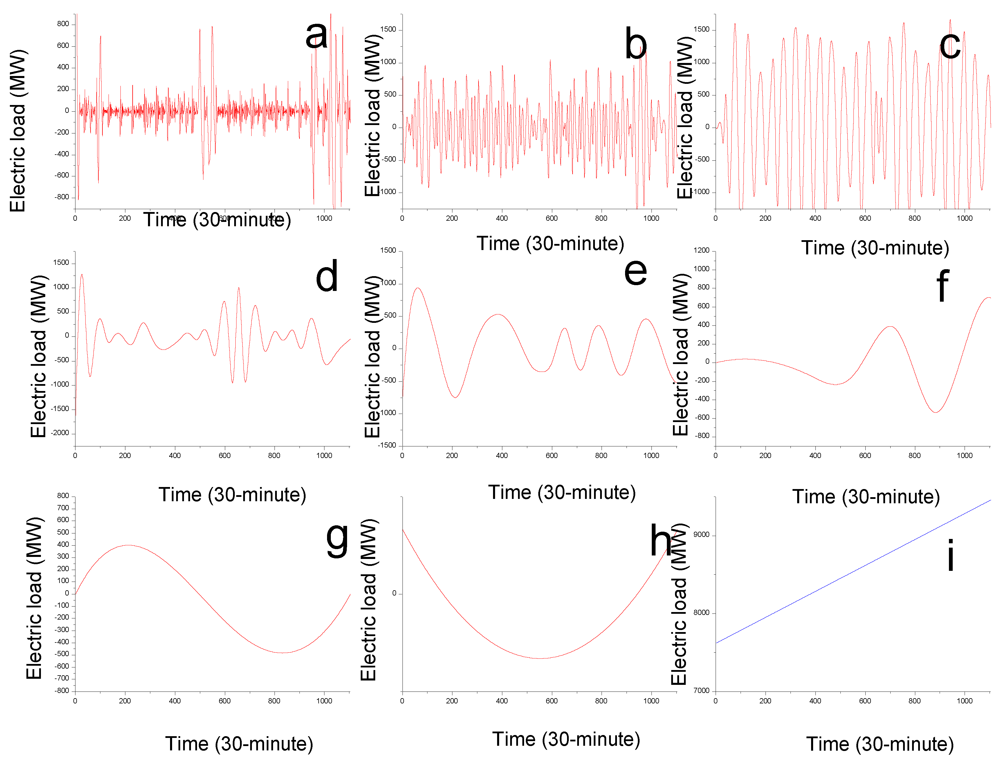
After decomposition by the EMD technique, it is obvious that the large sample data can be classified in nine terms. These nine decomposed terms are demonstrated in Figure 2a–i, in which the first term, Figure 2a, is the random term, the last term, Figure 2i, is the trend (residual) term. It is similar to the decomposed results for the small sample data, the detailed results of which can be seen in Fan et al. [35].

3.5. Forecasting Results by the SVR-PSO Model for Three Defined Items

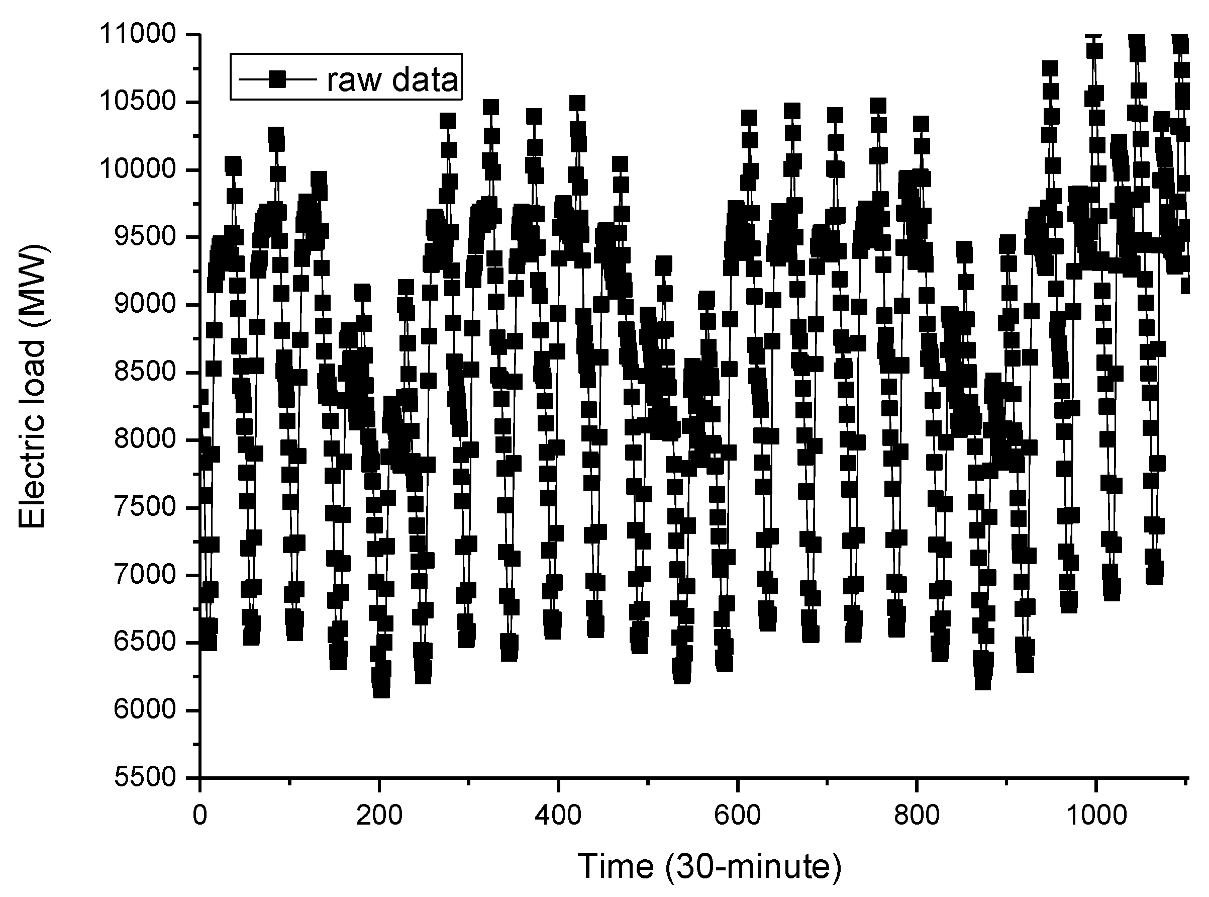
Figure 3 is the raw data of the large sample. It demonstrates the fluctuation characteristics, such as non-linearity and multiple peaks and valleys. The trend (residual) term is difficult to capture. The non-stationarity characteristics of data implies the dynamics between various time periods in the data sequence, which may change the correlation between the past time period and the future period. Thus, the dynamic changing process is unable to be dealt well only by a single time series analysis model. However, it is useful to apply the EMD technique to reduce the non-stationarity. In addition, the noisy level fluctuation also varies in different time periods in the time series data, particularly for the random term, which demonstrates the disturbing details of the continuous changes. A single time series model could encounter local under-fitting or over-fitting problems extracting features from different time periods with various noisy levels.
The SVR model is very adaptive to solve such continuous changing details of time series forecasting problems. To reduce the performance volatility with different parameters of the SVR model, the PSO algorithm is appropriate to optimize the combination of the parameters. Particularly, the rolling-based procedure [34], is employed in the training stage to assist the PSO algorithm to find the most appropriate parameters combination of an SVR model. Firstly, as mentioned above, the decomposed IMFs are defined to form the following items, A, B, C and D. These four items are simultaneously modeled by the SVR-PSO model, and the suitable parameter combination for the four items in the small and the large samples are illustrated in Table 1.
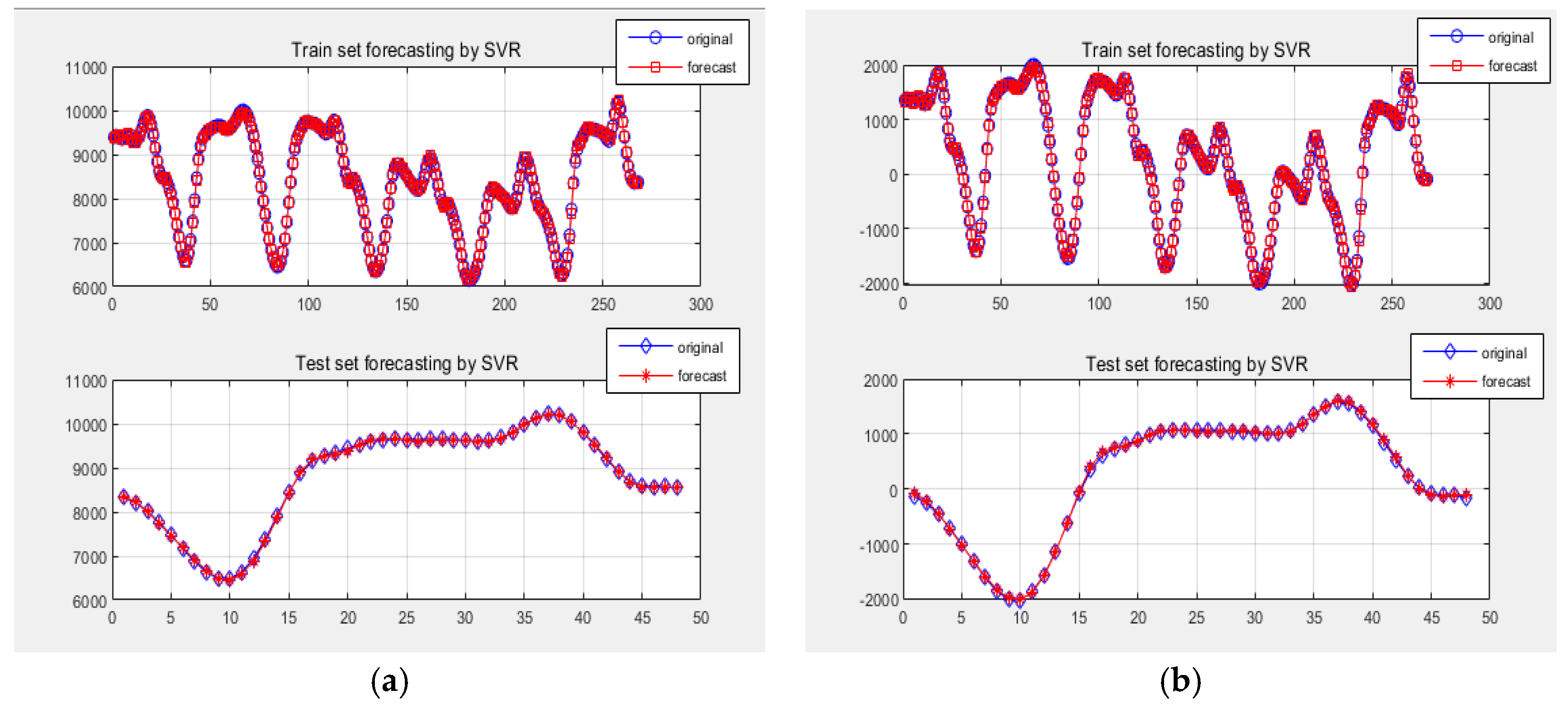
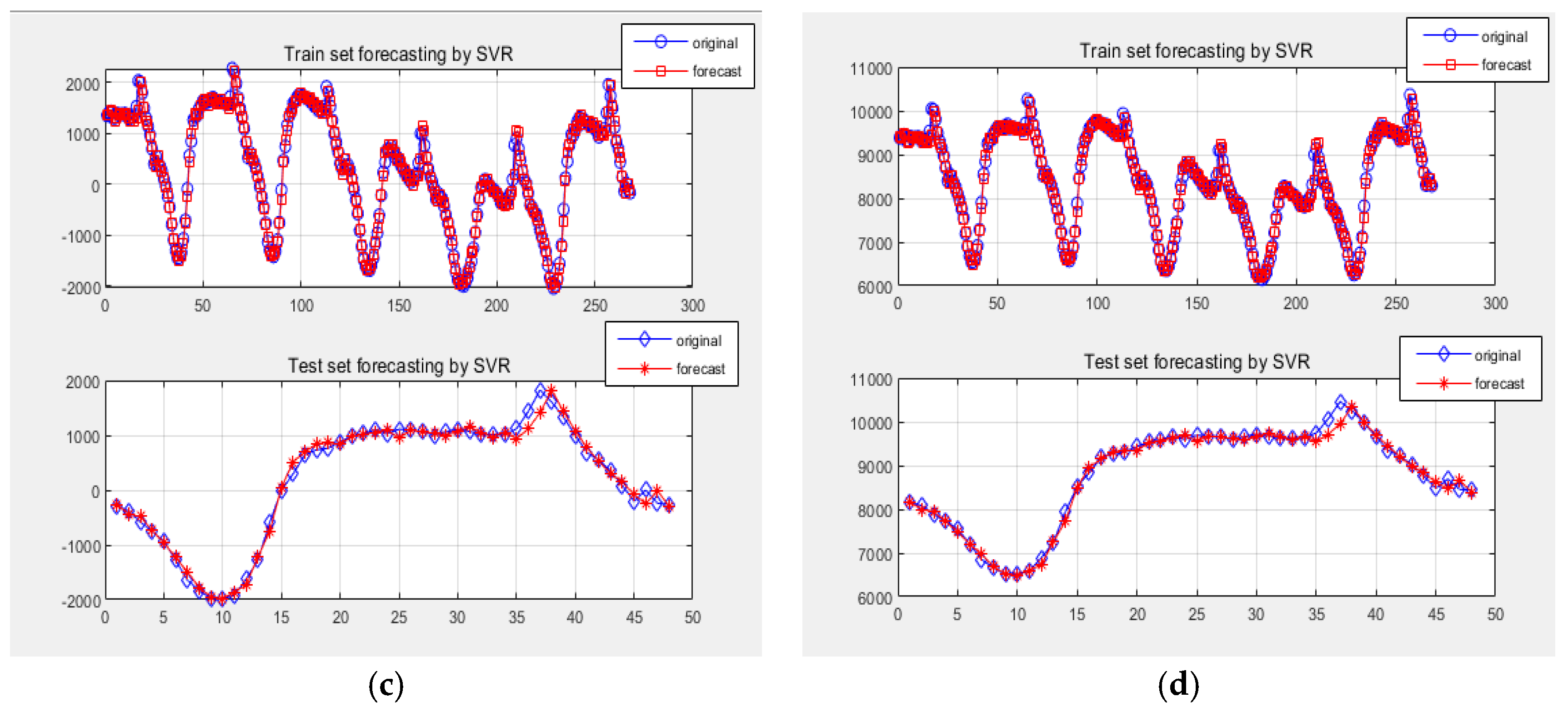
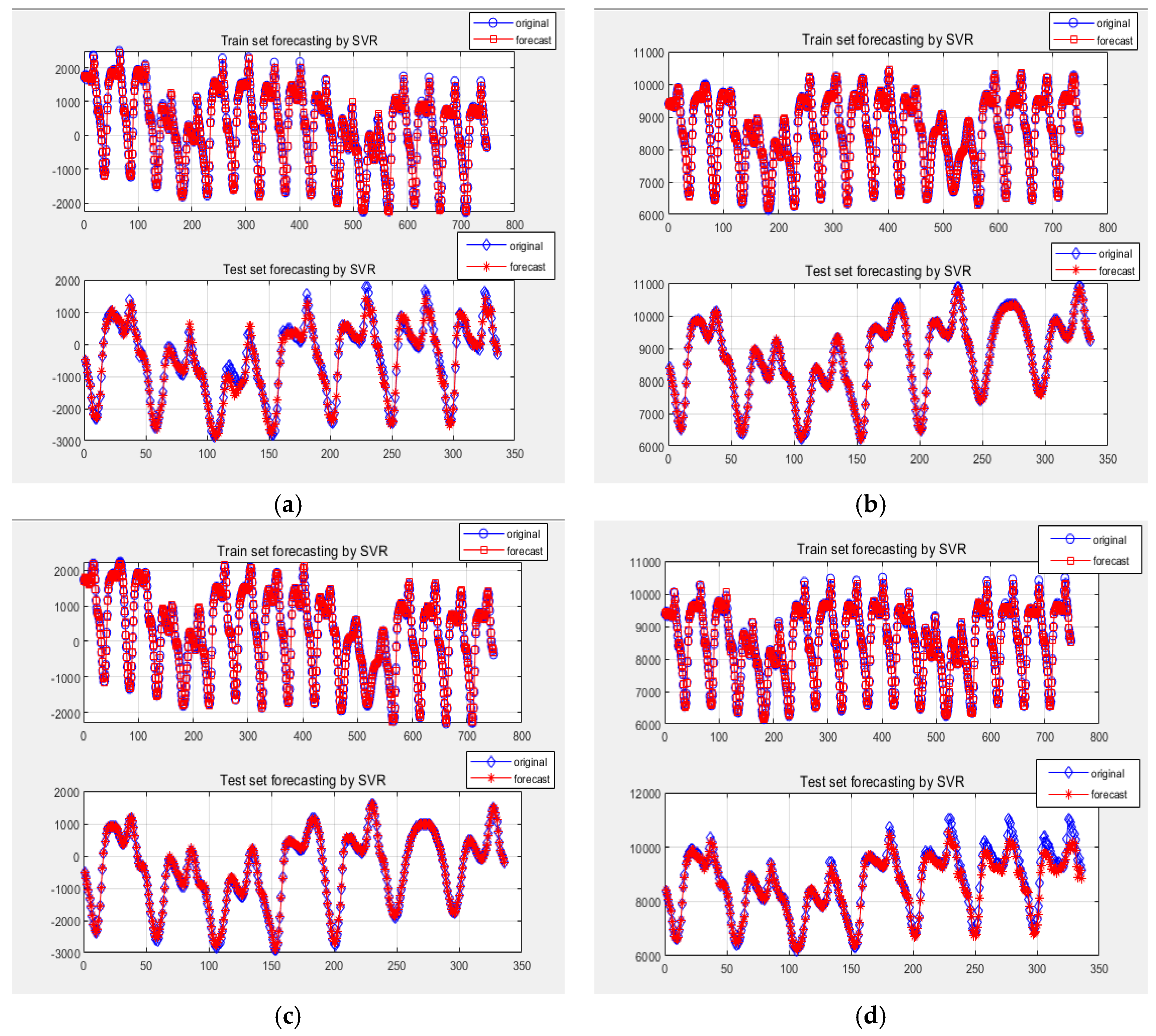
The performances for different defined items in the training and testing (forecasting) sets for the small and the large samples are demonstrated in Figure 4 and Figure 5, respectively.
The values of different forecasting indexes for different defined items in the training and testing stages for the small and the large samples are illustrated in Table 2. It is obviously that the forecasting performance of all items are outstanding, particularly for items A and B, whose forecasting accuracies are almost zero in terms of the square of RMSE. The results imply that the decomposition effects of the EMD technique are useful to increase the forecasting performance from the data composition side. In addition, the forecasting accuracy of the item D by the SVR-PSO model is also superior to the one achieved by the original SVR model. It also indicates that the optimization effects from the PSO algorithm are helpful to improve the forecasting accuracy from the parameter selection side.

3.6. Analyses of Forecasting Accuracy and the Relevant Applications

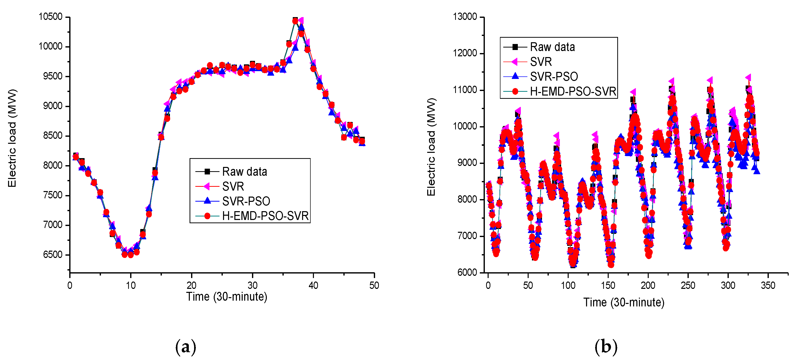
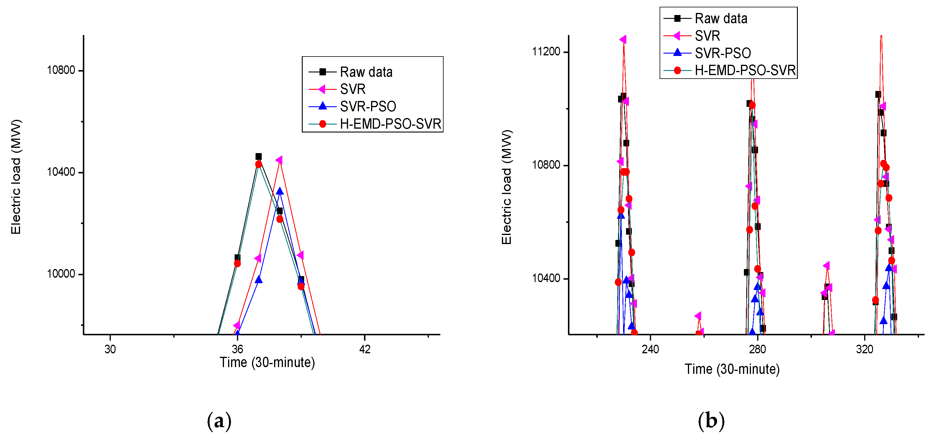
For the small sample, the forecasting results of the original SVR model, the SVR-PSO model, and the proposed H-EMD-SVR-PSO model are demonstrated in Figure 6a. It indicates that the forecasting curve of the proposed H-EMD-SVR-PSO model fits closer than other compared models. For the large sample, Figure 6b illustrates the forecasting results obtained from the proposed H-EMD-SVR-PSO model fits better than other compared models, particularly for those peak load values. In addition, from the local enlarged figure (Figure 7), the peak points of the small and the large samples demonstrate that the proposed H-EMD-SVR-PSO model can capture the mutative changes of the electric loads and can provide effective forecasting the reduced situation of electricity demand, thus, successfully reducing the losses of the power company.
Furthermore, the proposed H-EMD-SVR-PSO model has better generalization ability than other compared models. The comparison results are summarized in Table 3.
The proposed model is also compared with other alternative models proposed in references [32] and [35]. Firstly, the general observation in both samples is that the proposed model tends to fit closer to the actual electric load values with a smaller forecasting error. In addition, it is also found that proposed model outperforms the compared models (except EMD-SVR-AR and EMD-PSO-GA-SVR models) in terms of all the used forecasting accuracy indexes and the running times.
For the small sample, the proposed H-EMD-SVR-PSO model outperforms the original SVR model, SVR-PSO model [32], PSO-BP model [32], and SVR-GA model [35]. A slight forecasting accuracy index value behind the EMD-SVR-AR model [32] and EMD-PSO-GA-SVR model [35], i.e., the advantages of this kind of EMD-SVR-based models are superior to other SVR-based models, however, they are not much different in forecasting performance due to their use of the same hybridization structure. In the running time comparison, these kinds of EMD-SVR-based models often have high running speed, however, the running time would increase when the number of hybridizing techniques is large or the hybridized technique is very complicate in computing terms, such as the EMD-PSO-GA-SVR model which is the most time consuming among these three EMD-SVR-based models; on the contrary, when the number of hybridizing techniques is small or the hybridized technique is easy to model, such as the EMD-SVR-AR model is the most time saving among these EMD-SVR-based models.
On the other hand, from Table 3, the forecasting accuracy of the SVR-PSO model [32] is not outstanding when it is applied directly. This results from the interactive effects of the random term and the trend (residual) term, the so-called inherent non-linearity of the electric load data. After hybridizing with the EMD technique, the proposed H-EMD-SVR-PSO model is capable of capturing the inherent non-linearity by separately modeling these decomposed IMFs and these defined items (A, B, C and D). The forecasting performance of items A and B are significantly improved, which indicates that the inherent non-linearity of the electric load data can be effectively explained by the proposed model. In the other words, the proposed H-EMD-SVR-PSO model provides a very powerful tool to easily implement the electric load forecasting work.
The significance of the forecasting performance from the proposed H-EMD-SVR-PSO model should be further verified. The recommended statistical test by Derrac et al. [45] and Fan et al. [31], namely Wilcoxon signed-rank test is used to conduct the forecasting performance comparison among the proposed H-EMD-SVR-PSO model and the alternative models. The test is based on one-tail-test and is under two significance levels, α = 0.025 and α = 0.05. The test results are shown in Table 4. Clearly, the proposed H-EMD-SVR-PSO model significantly outperforms other compared models. In other words, the hybrid model leads to better accuracy and statistical interpretation.
Finally, some real life applications of the proposed methodology could be as followings. Via the EMD operation, (1) the random (stochastic) volatility term can be obviously revealed, which could be viewed as the microeconomic behavior; (2) the trend (residual) term is the inertial behavior, i.e., the general tendency of the economy, which could be viewed as the macroeconomic behavior; and (3) the middle term could be expressed from the unique economic behavior or production and living characteristics of each industry. Thus, the reason that the item A (the random term plus the middle term) could be well simulated during the modeling processes of the SVR-PSO model is that the characteristics of economic behaviors in each industry and their interactive influences (i.e., the random fluctuations) are in line with the modeling rules of the PSO algorithm (i.e., from random solution to adaptability). On the other hand, while the item B (the middle term plus the trend (residual) term) is characterizing, the SVR-based model (with the generalized linear capability in the feature space) can reveal the characteristics of economic behaviors along with the optimization processes of the PSO algorithm. Based on the observation from the above two items (items A and B), the proposed H-EMD-SVR-PSO model is obviously to have superior forecasting results, as shown in Table 2. In addition, the proposed model can be furtherly applied not only in electricity load forecasting, but also for the disclosure of other energy consumption behaviors or similar rules.

4. Conclusions

This paper proposes a novel H-EMD-SVR-PSO electric load forecasting model, by classifying the IMFs decomposed by the EMD technique into four different defined items (A, B, C and D). It is effective at overcoming the interactive effects of the random term and the trend (residual) term, and the inherent non-linearity of the electric load data. In addition, by hybridizing the PSO algorithm to optimize the parameter combination of the SVR model for these four items, respectively, it can effectively guarantee the better forecasting performance of each item by using the SVR-PSO model. Via two experiments with different sample sizes from the Australian market data, the proposed model has obtained significant forecasting results than other alternative models in the existed papers, such as original SVR, SVR-PSO, PSO-BP, SVR-GA, EMD-SVR-AR and EMD-PSO-GA-SVR models.
The results also verify the feasibility and the generalization capability of the EMD-SVR-based model to deal with the complicate interactions inherent in the electric load data. Various data characteristics of electric load are decomposed and identified by the employed EMD technique, which can guide researchers to select more suitable SVR-based forecasting models. For future research, the EMD-SVR-based model can be hybridized with other advanced classification tools to further improve the electric load forecasting accuracy.

Author Contributions

G.-F.F. and W.-C.H. conceived and designed the experiments; G.-F.F. performed the experiments and analyzed the data; W.-C.H. wrote the paper.

Funding

This paper is sponsored by the Academic and Technical Leader of Pingdingshan University, Program for Young Scholar of Pingdingshan University, and the support from Jiangsu Normal University (no. 9213618401), China.

Conflicts of Interest

The authors declare no conflict of interest.

References

  1. Xiao, L.; Shao, W.; Liang, T.; Wang, C. A combined model based on multiple seasonal patterns and modified firefly algorithm for electrical load forecasting. Appl. Energy 2016, 167, 135–153. [Google Scholar] [CrossRef]
  2. Hussain, A.; Rahman, M.; Memon, J.A. Forecasting electricity consumption in Pakistan: The way forward. Energy Policy 2016, 90, 73–80. [Google Scholar] [CrossRef]
  3. Tarsitano, A.; Amerise, I.L. Short-term load forecasting using a two-stage sarimax model. Energy 2017, 133, 108–114. [Google Scholar] [CrossRef]
  4. Boroojeni, K.G.; Amini, M.H.; Bahrami, S.; Iyengar, S.S.; Sarwat, A.I.; Karabasoglu, O. A novel multi-time-scale modeling for electric power demand forecasting: From short-term to medium-term horizon. Electr. Power Syst. Res. 2017, 142, 58–73. [Google Scholar] [CrossRef]
  5. Dudek, G. Pattern based local linear regression models for short term load forecasting. Electr. Power Syst. Res. 2016, 130, 139–147. [Google Scholar] [CrossRef]
  6. Vu, D.H.; Muttaqi, K.M.; Agalgaonkar, A.P. A variance inflation factor and backward elimination based robust regression model for forecasting monthly electricity demand using climatic variables. Appl. Energy 2015, 140, 385–394. [Google Scholar] [CrossRef] [Green Version]
  7. Wu, J.; Wang, J.; Lu, H.; Dong, Y.; Lu, X. Short term load forecasting technique based on the seasonal exponential adjustment method and the regression model. Energy Convers. Manag. 2013, 70, 1–9. [Google Scholar] [CrossRef]
  8. Maçaira, P.M.; Souza, R.C.; Oliveira, F.L.C. Modelling and forecasting the residential electricity consumption in Brazil with pegels exponential smoothing techniques. Procedia Comput. Sci. 2015, 55, 328–335. [Google Scholar] [CrossRef]
  9. Dong, Z.; Yang, D.; Reindl, T.; Walsh, W.M. Short-term solar irradiance forecasting using exponential smoothing state space model. Energy 2013, 55, 1104–1113. [Google Scholar] [CrossRef]
  10. De Oliveira, E.M.; Oliveira, F.L.C. Forecasting mid-long term electric energy consumption through bagging ARIMA and exponential smoothing methods. Energy 2018, 144, 776–788. [Google Scholar] [CrossRef]
  11. Takeda, H.; Tamura, Y.; Sato, S. Using the ensemble Kalman filter for electricity load forecasting and analysis. Energy 2016, 104, 184–198. [Google Scholar] [CrossRef]
  12. Scarpa, F.; Bianco, V. Assessing the quality of natural gas consumption forecasting: An application to the Italian residential sector. Energies 2017, 10, 1879. [Google Scholar] [CrossRef]
  13. Niu, D.X.; Shi, H.F.; Wu, D.D. Short-term load forecasting using Bayesian neural networks learned by hybrid Monte Carlo algorithm. Appl. Soft Comput. 2012, 12, 1822–1827. [Google Scholar] [CrossRef]
  14. Hippert, H.S.; Taylor, J.W. An evaluation of Bayesian techniques for controlling model complexity and selecting inputs in a neural network for short-term load forecasting. Neural Netw. 2010, 23, 386–395. [Google Scholar] [CrossRef] [PubMed]
  15. Bianco, V.; Cascetta, F.; Marino, A.; Nardini, S. Understanding energy consumption and carbon emissions in Europe: A focus on inequality issues. Energy 2019, 170, 120–130. [Google Scholar] [CrossRef]
  16. Kelo, S.; Dudul, S. A wavelet Elman neural network for short term electrical load prediction under the influence of temperature. Int. J. Electr. Power Energy Syst. 2012, 43, 1063–1071. [Google Scholar] [CrossRef]
  17. Ghofrani, M.; Ghayekhloo, M.; Arabali, A.; Ghayekhloo, A. A hybrid short-term load forecasting with a new input selection framework. Energy 2015, 81, 777–786. [Google Scholar] [CrossRef]
  18. Singh, P.; Dwivedi, P. Integration of new evolutionary approach with artificial neural network for solving short term load forecast problem. Appl Energy 2018, 217, 537–549. [Google Scholar] [CrossRef]
  19. Khwaja, A.S.; Zhang, X.; Anpalagan, A.; Venkatesh, B. Boosted neural networks for improved short-term electric load forecasting. Electr. Power Syst. Res. 2017, 143, 431–437. [Google Scholar] [CrossRef]
  20. Duan, Q.; Liu, J.; Zhao, D. Short term electric load forecasting using an automated system of model choice. Int. J. Electr. Power Energy Syst. 2017, 91, 92–100. [Google Scholar] [CrossRef]
  21. Karimi, M.; Karami, H.; Gholami, M.; Khatibzadehazad, H.; Moslemi, N. Priority index considering temperature and date proximity for selection of similar days in knowledge-based short term load forecasting method. Energy 2018, 144, 928–940. [Google Scholar] [CrossRef]
  22. Chaturvedi, D.K.; Sinha, A.P.; Malik, O.P. Short term load forecast using fuzzy logic and wavelet transform integrated generalized neural network. Int. J. Electr. Power Energy Syst. 2015, 67, 230–237. [Google Scholar] [CrossRef]
  23. Sadaei, H.J.; Guimarães, F.G.; da Silva, C.J.; Lee, M.H.; Eslami, T. Short-term load forecasting method based on fuzzy time series, seasonality and long memory process. Int. J. Approx. Reason. 2017, 83, 196–217. [Google Scholar] [CrossRef]
  24. Efendi, R.; Ismail, Z.; Deris, M.M. A new linguistic out-sample approach of fuzzy time series for daily forecasting of Malaysian electricity load demand. Appl. Soft Comput. 2015, 28, 422–430. [Google Scholar] [CrossRef]
  25. Hooshmand, R.A.; Amooshahi, H.; Parastegari, M. A hybrid intelligent algorithm based short-term load forecasting approach. Int. J. Electr. Power Energy Syst. 2013, 45, 313–324. [Google Scholar] [CrossRef]
  26. Lou, C.W.; Dong, M.C. A novel random fuzzy neural networks for tackling uncertainties of electric load forecasting. Int. J. Electr. Power Energy Syst. 2015, 73, 34–44. [Google Scholar] [CrossRef]
  27. Niu, M.; Sun, S.; Wu, J.; Yu, L.; Wang, J. An innovative integrated model using the singular spectrum analysis and nonlinear multi-layer perceptron network optimized by hybrid intelligent algorithm for short-term load forecasting. Appl. Math. Model. 2016, 40, 4079–4093. [Google Scholar] [CrossRef]
  28. Zhao, J.; Liu, X. A hybrid method of dynamic cooling and heating load forecasting for office buildings based on artificial intelligence and regression analysis. Energy Buildings 2018, 174, 293–308. [Google Scholar] [CrossRef]
  29. Yu, F.; Xu, X. A short-term load forecasting model of natural gas based on optimized genetic algorithm and improved BP neural network. Appl. Energy 2014, 134, 102–113. [Google Scholar] [CrossRef]
  30. Liu, N.; Tang, Q.; Zhang, J.; Fan, W.; Liu, J. A hybrid forecasting model with parameter optimization for short-term load forecasting of micro-grids. Appl. Energy 2014, 129, 336–345. [Google Scholar] [CrossRef]
  31. Fan, G.-F.; Peng, L.-L.; Hong, W.-C. Short term load forecasting based on phase space reconstruction algorithm and bi-square kernel regression model. Appl. Energy 2018, 224, 13–33. [Google Scholar] [CrossRef]
  32. Fan, G.; Wang, H.; Qing, S.; Hong, W.-C.; Li, H.-J. Support vector regression model based on empirical mode decomposition and auto regression for electric load forecasting. Energies 2013, 6, 1887–1901. [Google Scholar] [CrossRef]
  33. Geng, J.; Huang, M.L.; Li, M.W.; Hong, W.C. Hybridization of seasonal chaotic cloud simulated annealing algorithm in a SVR-based load forecasting model. Neurocomputing 2015, 151, 1362–1373. [Google Scholar] [CrossRef]
  34. Hong, W.-C.; Dong, Y.; Lai, C.-Y.; Chen, L.-Y.; Wei, S.-Y. SVR with hybrid chaotic immune algorithm for seasonal load demand forecasting. Energies 2011, 4, 960–977. [Google Scholar] [CrossRef]
  35. Fan, G.-F.; Peng, L.-L.; Zhao, X.; Hong, W.-C. Applications of hybrid EMD with PSO and GA for an SVR-based load forecasting model. Energies 2017, 10, 1713. [Google Scholar] [CrossRef]
  36. Hong, W.-C.; Dong, Y.; Zhang, W.; Chen, L.-Y.; Panigrahi, B.K. Cyclic electric load forecasting by seasonal SVR with chaotic genetic algorithm. Int. J. Electr. Power Energy Syst. 2013, 44, 604–614. [Google Scholar] [CrossRef]
  37. Ju, F.-Y.; Hong, W.-C. Application of seasonal SVR with chaotic gravitational search algorithm in electricity forecasting. Appl. Math. Model. 2013, 37, 9643–9651. [Google Scholar] [CrossRef]
  38. Li, M.; Hong, W.-C.; Kang, H. Urban traffic flow forecasting using Gauss-SVR with cat mapping, cloud model and PSO hybrid algorithm. Neurocomputing 2013, 99, 230–240. [Google Scholar] [CrossRef]
  39. Chen, R.; Liang, C.; Hong, W.-C.; Gu, D. Forecasting holiday daily tourist flow based on seasonal support vector regression with adaptive genetic algorithm. Appl. Soft Comput. 2015, 26, 435–443. [Google Scholar] [CrossRef]
  40. Huang, B.; Kunoth, A. An optimization based empirical mode decomposition scheme. J. Comput. Appl. Math. 2013, 240, 174–183. [Google Scholar] [CrossRef]
  41. An, X.; Jiang, D.; Zhao, M.; Liu, C. Short-term prediction of wind power using EMD and chaotic theory. Commun. Nonlinear Sci. Numer. Simul. 2012, 17, 1036–1042. [Google Scholar] [CrossRef]
  42. Fan, G.; Qing, S.; Wang, S.Z.; Hong, W.C.; Dai, L. Study on apparent kinetic prediction model of the smelting reduction based on the time series. Math. Probl. Eng. 2012, 720849. [Google Scholar] [CrossRef]
  43. Premanode, B.; Toumazou, C. Improving prediction of exchange rates using Differential EMD. Expert Syst. Appl. 2013, 40, 377–384. [Google Scholar] [CrossRef]
  44. Dong, Y.; Zhang, Z.; Hong, W.-C. A hybrid seasonal mechanism with a chaotic cuckoo search algorithm with a support vector regression model for electric load forecasting. Energies 2018, 11, 1009. [Google Scholar] [CrossRef]
  45. Derrac, J.; García, S.; Molina, D.; Herrera, F. A practical tutorial on the use of nonparametric statistical tests as a methodology for comparing evolutionary and swarm intelligence algorithms. Swarm Evol. Comput. 2011, 1, 3–18. [Google Scholar] [CrossRef]
Figure 1. The full flowchart of the proposed H-EMD-SVR-PSO model.
Energies 12 01093 g001
Figure 2. The decomposed items for the large sample data. (a) IMF1 (the random term); (b) IMF2 (the middle term 1); (c) IMF3 (the middle term 2); (d) IMF4 (the middle term 3); (e) IMF5 (the middle term 4); (f) IMF6 (the middle term 5); (g) IMF7 (the middle term 6); (h) IMF8 (the middle term 7); and (i) IMF9 (the trend (residuals) term).
Energies 12 01093 g002
Figure 3. The raw data of the large sample data.
Energies 12 01093 g003
Figure 4. Comparison the forecasting results for different defined items by the SVR-PSO model (the small sample; one-day ahead forecasting on 8 May 2007). (a) Item A: the random term + the middle term; (b) Item B: the middle term + the trend (residual) term; (c) Item C: the middle term; (d) Item D: A + B − C (all IMFs, i.e., complete decomposed effects).
Energies 12 01093 g004aEnergies 12 01093 g004b
Figure 5. Comparison the forecasting results for different defined items by the SVR-PSO model (the large sample; one-week ahead forecasting on 18 to 24 May 2007). (a) Item A: the random term + the middle term; (b) Item B: the middle term + the trend (residual) term; (c) Item C: the middle term; (d) Item D: A + B − C (all IMFs, i.e., complete decomposed effects).
Energies 12 01093 g005
Figure 6. Comparison of the forecasting results among the H-EMD-SVR-PSO model and other models. (a) The small sample; (b) The large sample.
Energies 12 01093 g006
Figure 7. The local enlargement (peak) comparison of the H-EMD-SVR-PSO model and other models. (a) The small sample; (b) The large sample.
Energies 12 01093 g007
Table 1. The optimized parameters of the SVR-PSO model for different items in both samples.
Sample Size/Defined ItemsThe Parameters of an SVR Model
σ C ε
The small sample data
Item A: the random term + the middle term0.14890.0022
Item B: the middle term + the trend (residual) term0.14880.0020
Item C: the middle term0.15910.0025
Item D: A + B − C (all IMFs, i.e., complete decomposed effects)0.15920.0025
The large sample data
Item A: the random term + the middle term0.18950.0011
Item B: the middle term + the trend (residual) term0.18960.0011
Item C: the middle term0.20980.0013
Item D: A + B − C (all IMFs, i.e., complete decomposed effects)0.20980.0012
Table 2. Summary of the forecasting results for each defined items.
Forecasting Accuracy IndexesThe Defined Items
Item A (by SVR-PSO)Item B (by SVR-PSO)Item C (by SVR-PSO)Item D (by SVR-PSO)Item D (by SVR)
The Small Sample
RMSE 2 (training stage)0.00019360.00016350.00290.00090.0021
RMSE 2 (testing stage)0.00018060.00016410.00330.00110.0026
R (training stage)0.99930.99950.98880.98840.9871
R (testing stage)0.99940.99950.98670.98810.9890
The Large Sample
RMSE 2 (training stage)0.00012800.00010900.00070.00070.0012
RMSE 2 (testing stage)0.00022810.00028140.00330.00960.0099
R (training stage)0.99940.99940.99620.99650.9916
R (testing stage)0.99920.99910.99820.97560.9912
Table 3. Summary of results of the forecasting models.
Compared ModelsMAPERMSEMAERunning Time (s)
The Small Sample
Original SVR [32]11.70145.8710.92180.4
SVR-PSO [32]11.41145.6910.67165.2
PSO–BP [32]10.91142.2610.14159.9
SVR-GA [35]13.52150.3811.88171.3
EMD-SVR-AR [32]9.86117.169.1080.7
EMD-PSO-GA-SVR [35]9.09123.389.19135.7
H-EMD-SVR-PSO10.01125.389.75120.5
The Large Sample
Original SVR [32]12.88181.6212.05116.8
SVR-PSO [32]13.50271.4313.07192.7
PSO–BP [32]12.24175.2411.36163.1
SVR-GA [35]14.31183.5715.31195.7
EMD-SVR-AR [32]5.10134.209.82162.0
EMD-PSO-GA-SVR [35]3.92142.419.04179.1
H-EMD-SVR-PSO5.83130.179.56167.4
Table 4. Wilcoxon signed-rank test.
Compared ModelsWilcoxon Signed-Rank Test
α = 0.025; W = 4α = 0.05; W = 6
The Small Sample
H-EMD-SVR-PSO vs. Original SVR3 *3 *
H-EMD-SVR-PSO vs. SVR-PSO2 *2 *
H-EMD-SVR-PSO vs. PSO–BP2 *3 *
H-EMD-SVR-PSO vs. SVR-GA2 *3 *
H-EMD-SVR-PSO vs. EMD-SVR-AR64 *
H-EMD-SVR-PSO vs. EMD-PSO-GA-SVR68
The Large Sample
H-EMD-SVR-PSO vs. Original SVR3 *2 *
H-EMD-SVR-PSO vs. SVR-PSO3 *2 *
H-EMD-SVR-PSO vs. PSO–BP3 *2 *
H-EMD-SVR-PSO vs. SVR-GA3 *2 *
H-EMD-SVR-PSO vs. EMD-SVR-AR62 *
H-EMD-SVR-PSO vs. EMD-PSO-GA-SVR64 *
Note: * denotes that the H-EMD-SVR-PSO model significantly outperforms other alternative models.