Coupling Exergy with the Emission of Greenhouse Gases in Bioenergy: A Case Study Using Biochar

Abstract

The loss in the quality of energy throughout any process can be assessed by the thermodynamics magnitude related to its entropic performance—the exergy. This indicator has been suggested as an environmental index, as an alternative to life cycle assessment (LCA), which is a classic tool for this purpose. This study assesses the potential of coupling the life cycle approach and exergy in a bioenergy supply chain environmental performance characterization, examining two scenarios in the sugarcane agroindustry. The first one, the reference scenario, is a classical production, and the second includes the returning of a portion of residual biomass from the plant, in the form of biochar, to agricultural soil. The use of biochar engendered an increase in sugarcane productivities and a reduction of nitrous oxide emissions. These changes resulted in scenarios 1 and 2, reducing the exergy destroyed from 390 to 355 MJ/MJ ethanol (9.0%) and decreasing the greenhouse gases emissions (GHG) from 11.8 to 11.0 g CO_2-equivalent/MJ ethanol (6.8%). The latter represents an improvement in the use of carbon. A sensitivity analysis showed that the effect of changing productivity was quite significant: The exergy showed a sensitivity of −0.49, and in total emissions, this figure was slightly lower, at −0.41. By changing the emissions of N₂O in the soil, the sensitivity of exergy was almost null, and the total emissions were 0.077.

1. Introduction

Since the beginning of the 20th century, the world’s population has increased more than four-fold, increasing from 1.7 to 7 billion inhabitants. At the same time, there was a 100-fold increase in industrial production and a 50-fold increase in fossil fuel consumption, reaching 10,700 MTOE (million tons of oil equivalent) in 2016 [1]. More than one decade before, Graedel and Allenby [2] already pointed out that such consumption, either by the finiteness of natural resources or due to the consequential damage, has shown to be not sustainable in relation to the environment. The old industrial model, focused on production (and productivity), has somehow met such demands, although in an immediate manner. A new model has emerged, which is economically and socially feasible, as well as environmentally sustainable.

In order to allow for the development of this new industrial model, it is necessary to quantify the environmental impacts related to any processes, enabling a comparison of possible corrections, in which exergy can be of use. The use of the exergetic method, which, according to Kotas [3], is a relatively new alternative thermodynamic analysis based on the concept of exergy, is loosely defined as a universal measure of the work potential or quality of different forms of energy in relation to a given environment. Originally considered a technical working capacity or available energy, the Slovenian Zoran Rant, in a scientific meeting in 1953, suggested the term exergy to differentiate from energy [4].

Still, in the 1970s, Wall [5] proposed exergy as a useful concept in the management of resources. Rifkin and Howard [6] later claimed that both industrial systems and ecological processes materials and consume energy, like an economic system, and thermodynamics provides entropy as a thermodynamic property, which allows these transformations to be addressed. In the same way, Cornelissen [7] mentions that the exergetic analysis, originally applied in improving the efficiency of thermal machines, is an important tool for addressing the environmental effects associated with resource depletion as well as GHG emissions, especially those related to non-renewable energy sources. However, it is worth mentioning that [4] pointed out that exergy cannot be considered a good environmental performance indicator, which is qualitatively correct but incorrect quantitatively, but this is not the only approach of this study.

In this sense, Szargut et al. [8] proposed the concept of cumulative exergy consumption (CExC), which uses, within the life cycle of a product, the accumulated exergy, not only of energy flows but also of material inputs of the process, such as fuels, minerals or gases. Later, Dewulf et al. [9] extended the exergy analysis so that it could also include natural resources, extracted from ecosystems, such as solar radiation, among other things, through the CEENE methodology (cumulative exergy extraction from the natural environment), which studies the impact of resource accounting during a life-cycle assessment. In the specific case of bioproducts, this methodology accounts for exergy within a life cycle approach, taking into consideration the exergy of solar irradiation necessary to produce the initial biomass, thus extending the scope of the production chain from the cradle to the grave.

In such a context, LCA (life cycle assessment), which evolved from its origins in energy analysis, in the 1960s and 1970s, to a broadly used tool for determining the impacts of products or systems on various environmental and resource issues, has emerged as a new methodology to meet this need. With its broad life cycle approach, applied to the characterization of the supply chains, this environmental performance diagnostic tool is being widely used in the evaluation and quantification of potential environmental impacts of products or systems [10].

Within the combined context of bioenergy supply chains and the efficient use of resources, in which carbon is the fundamental resource, the main goal of this research is to comparatively assess the life cycle exergy consumption of an agro-industrial system of ethanol production and its GHG emissions.

2. Materials and Methods

The methodology includes the characterization of a case study in the bioenergy sector, namely, sugarcane-based ethanol production, coupled with a thermodynamic variable that represents the exergy extraction (CEENE—cumulative exergy extraction from the natural environment), with GHG emissions.

Exergy and emissions, as well as the relationship between them, were treated in two scenarios. Scenario 1, which is the reference system (RS), describes a sugarcane, typical for ethanol in the southwestern region of Brazil, calculated from the inventory reported by Macedo et al. [11], whose data were adjusted and/or updated, as presented in

Table 1. Reference values used in the calculation of inventory.

Variable	Value	Unity	Description
Carb_ethanol	0.4957	dimensionless	Carbon in hydrated ethanol (calculated)
Rat_co2carb	3.666	dimensionless	Mass ratio CO2 mass carbon (calculated)
Ex_co2	0.45	MJ/kg	Exergy of carbon dioxide [8]
Ex_h2so4	1.11	MJ/kg	Exergy of sulfuric acid [8]
Ex_k2o5	4.40	MJ/kg	Exergy of fertilizer K2O [8]
Ex_naoh	0.18	MJ/kg	Exergy of caustic soda [8]
Ex_nh3	19.9	MJ/kg	Exergy of ammonia [8]
Ex_p2o5	2.91	MJ/kg	Exergy of fertilizer P2O5 [8]
Ex_sdl	0.08	MJ/kg	Exergy of seedlings [8]
Ex_ww	0.72	MJ/kg	Exergy of whitewash [8]
App_k_ha	100.0	kg/ha	Annual average application rate of K2O [11]
App_ls	0.65	kg/SCT 1	Annual rate of limestone application [11]
App_n_ha	58.3	kg/ha	Annual average application rate of fertilizer N [11]
App_p_ha	36.7	kg/ha	Annual average application rate of P2O5 [11]
En_h2so4	3.093	MJ/SCT 1	Energy for the production of H2SO4 [11]
En_herb	11.24	MJ/SCT 1	Energy for the application of herbicides [11]
En_k2o	6.69	MJ/kg	Energy for the production of fertilizer K2O [11]
En_ls	7.13	MJ/SCT 1	Energy for the application of limestone [11]
En_n	61.45	MJ/kg	Energy for the production of fertilizer N [11]
En_p	9.61	MJ/kg	Energy for the production of fertilizer P2O5 [11]
En_sdl	5.88	MJ/SCT 1	Energy for the application of seedlings [11]
Rea_n_n	0.01	dimensionless	Reason N diminished N used in fertilization [11]
Bagasse_sct	270.0	kg/SCT 1	Bagasse mass 50% wet [19]
Prod_cane	70.0	SCT/ha	Productivity of sugarcane [19]
Prod_ethanol	88.0	L/SCT 1	Productivity of hydrated ethanol [19]
Diesel_dens	0.85	kg/L	Diesel density [20]
EF_diesel_kg	3.7	kg CO2-equivalent/kg Diesel	Diesel emission factor [20]
EF_fuel_mj	0.07735	kg CO2-equivalent/MJ	Emission factor of fuel oil [20]
Ethanol_dens	0.79	kg/L	Hydrated ethanol density [20]
Ex_diesel	42.28	MJ/kg	Exergy of diesel ≈ LHV [20]
Ex_dry_bagasse	18.90	MJ/kg	Dry bagasse exergy [21]
Ex_ wet_bagasse	9.89	MJ/kg	Exergy of bagasse that is 50% wet [22]
Ex_biochar	16.00	MJ/kg	Exergy of bagasse biochar [23]
Ex_cane	5.76	MJ/kg	Exergy of sugarcane [24]
Ex_ethanol	27.64	MJ/kg	Exergy of hydrated ethanol [24]
Ex_straw	12.97	MJ/kg	Exergy of straw that is 15% wet [25]
Diesel_ctr	0.85	kg/SCT 1	Diesel consumed in cane transport [26]
Diesel_oah	0.76	kg/SCT 1	Diesel consumed in agricultural operations and harvest [26]
Efic_KVA	0.28	dimensionless	Electricity generation thermal efficiency [26]
Port_straw	0.5	dimensionless	Portion of straw removed from the field for industry [26]
Straw_sct	165.0	kg/SCT 1	Amount of straw mass that is 15% wet [26]
Pot_n2o	265.0	dimensionless	Potential greenhouse effect of nitrous oxide [27]
Sol_rad	16.0	MJm−2day−1	Average annual solar radiation, SE, Brazil [27]

¹ Sugarcane ton.

, with appropriate references. Scenario 2 describes the changes due to the reusing of the industrial waste filtercake, which, after drying and pyrolysis, is transformed into biochar. These changes affect some items of the inventory, detailed in Table 1, thus altering both exergy consumption and GHG emissions.

Exergy is divided into four parts: potential, which is associated with a potential difference (X_po) that can be gravitational or even magnetic; kinetics (X_ki), which is associated with motion (speed); Physics (X_ph), which occurs as a result of differences in temperature and pressure, with respect to the environment and chemistry (X_ch), which are due to differences in the chemical composition between the initial and final states [3].

Exergy requires a reference level for its final state, which is considered dead when modified matter is under an equilibrium with the reference environment. As for physical exergy, both references, temperature and pressure, are described, with a zero index in the form of T₀ and P₀, standardized in 298 K and 1 bar, respectively [8]. Similarly, enthalpy (H₀) and entropy (S₀) refer to this same condition of T₀ and P₀. Thus, the physical exergy can be calculated according to Equation (1).

$$X_{ph}=H-H_0-T_0\left(S-S_0\right)=\Delta H_{ph}-T_0\Delta S_{ph}$$

(1)

where X: physical exergy (J); H(J): enthalpy of the flow in the process under T, P conditions; H₀ (J): enthalpies of the flow under the T₀, P₀ reference conditions; S (JK⁻¹): entropy of the flow in the process under conditions T, P; S₀ (JK⁻¹): entropy of the flow in the process under T₀, P₀ conditions; T₀ (K): reference temperature; and P₀: reference pressure (100 KPa).

Concerning chemical exergy, the level or reference state for most elements is where they present themselves in the most oxidized or chlorinated form. When in balance with the atmosphere, hydrosphere and crust, these elements, under such conditions, are taken as the reference state, with their state, concentration and composition defined, that is, the exergy value of a chemical compound is determined by comparing it with the standard condition of this compound in the terrestrial biosphere [12,13,14]. The general formulation proposed by Szargut [12] is presented in Equations (2) and (3).

$$X_{CH}={\displaystyle \sum }_i{n}_i{\tilde{b}}_{ch,i}$$

(2)

where the exergy part of the molar component $i,{\tilde{b}}_{ch,i}$ is calculated by Equation (3).

$${\tilde{b}}_{ch,i}={\tilde{b}}_{ch,i}^0+R{T}_{0}ln{x}_i{\phi }_i$$

(3)

where ${\tilde{b}}_{ch,i}^0$: molarpart of i component exergy under the T₀, P₀ (Jmol⁻¹) reference conditions; R: the ideal gas constant (Jmol⁻¹ K⁻¹); x_i: molar composition of i component; and φ_i: fugacity coefficient of i component.

According to Maes and Passel [14], there are two possible approaches for including solar irradiation in the exergy calculation. The first one is to include it only indirectly, only accounting for the biomass provided to the industrial process [15], and a second one, more comprehensive and inclusive approach, accounting for all solar irradiation necessary to produce biomass, which is the expanded concept of the cumulative exergy consumption (CExC) of Szargut et al. [8] and the entitled CEENE methodology (cumulative exergy extraction from the natural environment), assessing all kinds of resources that are excluded from the natural ecosystem, proposed by Dewulf et al. [9]. The value of CEENE, normalized here by megajoules of the ethanol unit, is described in Equation (4).

$$\mathrm{CEENE}={\displaystyle \sum }_{i=1}^n{\mathrm{ExC}}_{i\left(\mathrm{in}\right)}-{\displaystyle \sum }_{i=1}^n{\mathrm{ExC}}_{i\left(\mathrm{out}\right)}$$

(4)

where CEENE: the process (MJ/MJ ethanol); ∑ExC_i (in): sum of the accumulated exergy of n inputs (MJ/MJ ethanol); and ∑ExC_i (out): sum of the accumulated exergy of n outputs (MJ/MJ ethanol).

GHG emissions were also normalized by megajoules of ethanol, and this was accounted for in the general Equation (5).

$${\epsilon }_{\mathrm{GHG}}={\displaystyle \sum }_{i=1}^n{\epsilon }_i$$

(5)

where ε_GHG: greenhouse gas emissions of the process (g CO_2-equivalent/MJ ethanol); and ε_i: sum of the emissions of n inputs/products.

The ratio of these quantities, which is between CEENE and GHG emissions, in the considered scenarios, is already presented in Equation (6).

$${\kappa }_j=\frac{{\mathrm{CEENE}}_j}{{\epsilon }_{\mathrm{GHG}-j}}$$

(6)

where ${\kappa }_j:$ CEENE and emissions ratio in scenario j (in MJ/kg CO_2-equivalent); CEENE_j: Cumulative Exergy Extraction from the Natural Environment in scenario j (MJ/MJ ethanol); and ε_GHG-j: GHG emissions in scenario j (kg CO_2-equivalent/MJ ethanol).

In general, the use of this same ratio, when altering n possible input variables, can be presented as a dependent Y function, as shown in Equation (7).

$$Y\left(X_1,X_2\dots .X_n\right)=\frac{\mathrm{CEENE}\left(X_1,X_2\dots X_n\right)}{{\epsilon }_{\mathrm{GHG}}\left(X_1,X_2\dots .X_n\right)}$$

(7)

where $Y$: variable that represents the rate of CEENE and GHG emissions (MJ/g CO_2-equivalent); X₁, X₂ … X_n: input variables; CEENE: (MJ/MJ ethanol); and ε: GHG emissions (g CO_2-equivalent/MJ ethanol).

When addressing the sensitivity issue of variables, in the study, it was briefly indicated that, when comparing the output dependent variable behavior, it is usual to change the input variable value from 0 to 200% of its base or reference value. The behavior between the input and output variation is what makes it possible to quantify the sensitivity of this variable, both in relation to the other variable and the other points of the scanning [16,17].

Regarding sensitivity, when there is an explicit algebraic relationship, describing the relationship between an independent X_i variable and a dependent Y variable, this analysis is easy to carry out, and in this case, the Φ_i sensitivity coefficient for an independent variable in the study can be calculated on the basis of an X_i variable. For small changes in the input parameters, the partial derivative can be approximated as a finite difference, where non-linearity is neglected, and the partial derivative can be approximated in numerical form as Equation (8).

$${\Phi }_i=\frac{\%\Delta Y}{\%\Delta X_i}$$

(8)

where ${\Phi }_i$: sensitivity in X_i; % ΔY: percentage variation of Y magnitude; and % ΔX_i: percentage variation of X_i magnitude.

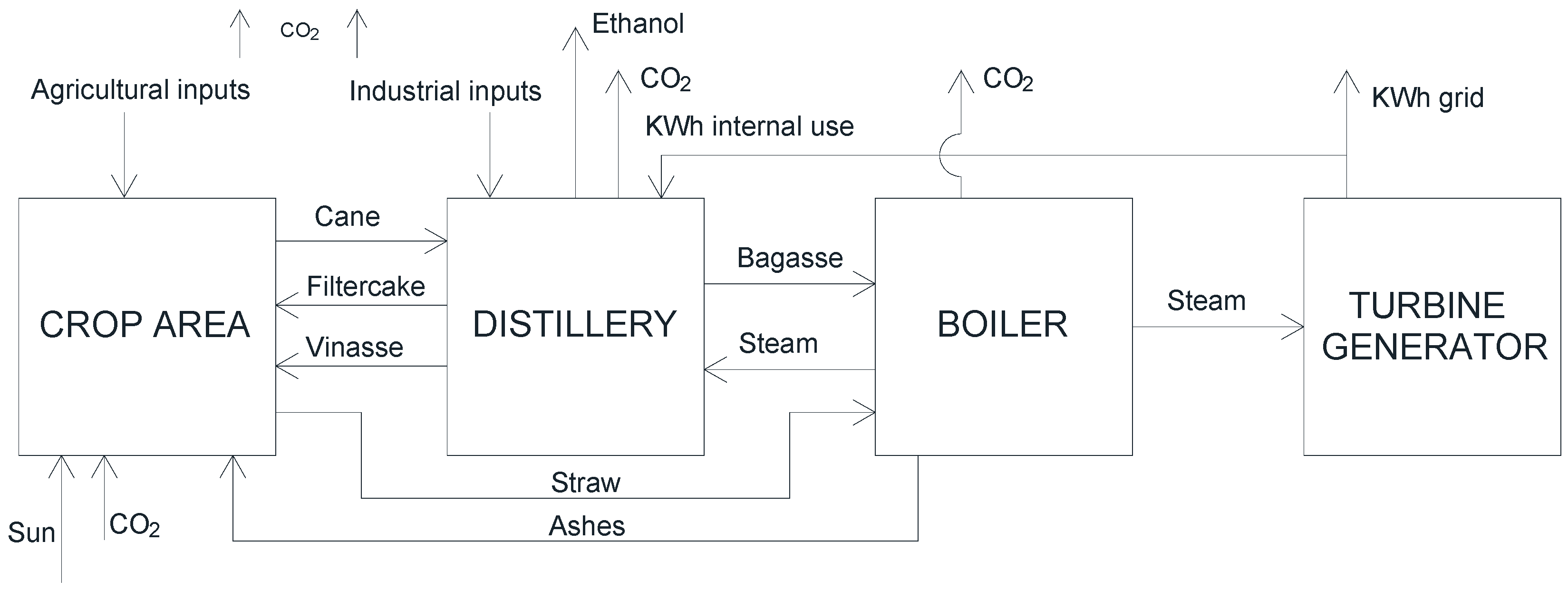
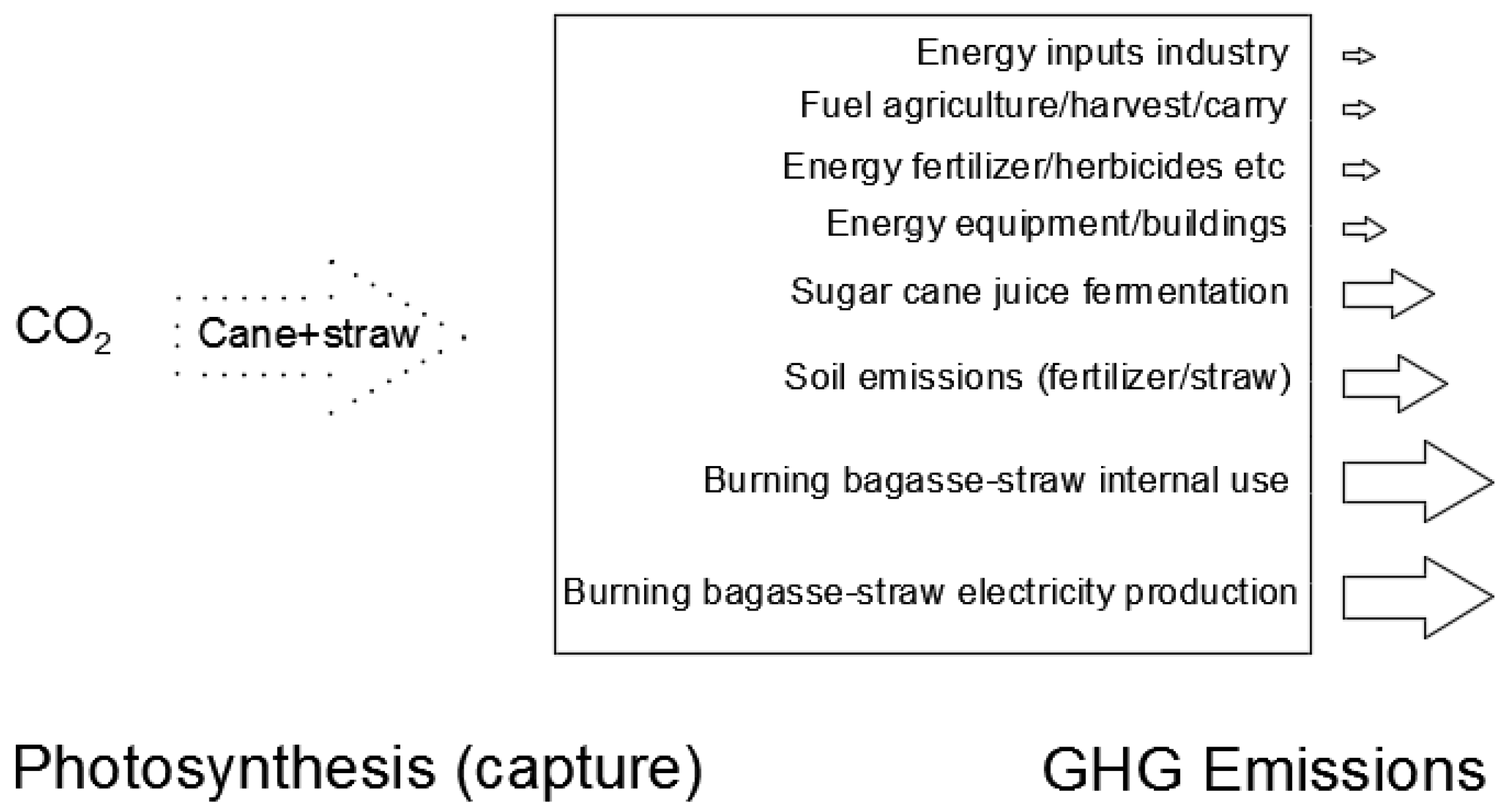
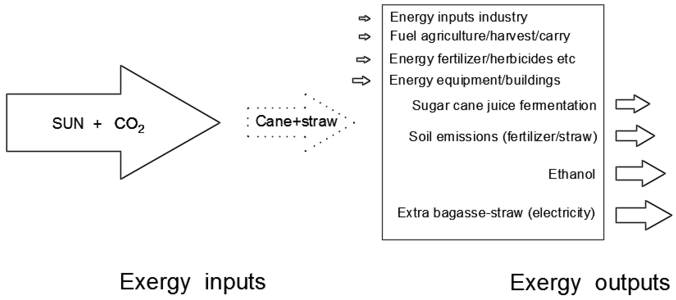
2.1. Bioenergy Systems, GHG and Exergy

The simplified flowchart of the process in the sugar ethanol sector, which was the basis of this study, is presented in Figure 1. Within the limits of this system, composed of both agricultural and industrial parts, are catalogued as both emissions and exergy flows.

It is highlighted that the main exergy flow entering the system is sunlight, and the main outputs are ethanol and electricity, which are exported to the plant. The latter was produced from steam from bagasse and straw. All emissions throughout the process were catalogued, from the capture of carbon in photosynthesis, turning it into sugarcane and straw, until its return to the atmosphere during the cycle.

The limits of the system under study are the limits of the agro-industry itself, from agricultural biomass production to industrial processing. In sucroenergy, the vinasse, ash and filtercake that were returned to the soil, without any treatment, have not been accounted for.

The exergy outcomes of CEENE and the associated GHG emissions, by ethanol megajoules, will be grouped at the same levels, as proposed by Szargut et al. [8], as follows:

• Level 1: Direct inputs, considered beyond the Sun, fuel consumption and the electric energy occasionally taken from an external source;
• Level 2: Indirect energy inputs, where it is added to the first level of the energy/emissions associated with the production of other inputs, either by the crop or through the manufacturing process;
• Level 3: The energy/emissions, related to the production and maintenance of equipment and installations, added to the previous levels. In this study, level 3 was used.

Emissions during biofuel production, with which this study is concerned, at the levels already mentioned, as well as the carbon cycle in sucroenergy, are represented in a summarized way in Figure 2. At the entrance, the carbon photosynthesis capture is represented, and at the exit, both the biotic and non-biotic carbon are represented. Non-biotic carbon-related emissions, as well as those that occur during the use of soil, represented by nitrogenous fertilizer’s N₂O, are the agents considered in this comparative LCA, that is, the biotic cycle is considered to be neutral.

Exergy inputs are grouped in the same way as the emissions, and their calculations were carried out in accordance with the aforementioned CEENE Equation (4). In Figure 3, the exergy inputs/products to the sucroenergy sector are briefly presented, both the high (energy drinks) and low exergy. In the case of fertilizers, accumulated exergy is calculated by the sum of the exergy consumed during production and by the chemical exergy present in the fertilizer itself (input), as well as the exergy of nitrous oxide emissions. The main exergy output of the bioenergy system is the ethanol itself, but there is also a large contribution of bagasse biomass and surplus straw to the production of electricity since the internal usage is irreversible in the process.

All the calculation presented in the course of this work were carried out, in vector form, in the numerical software, Scilab [18], from the values listed in Table 1. From the dataset of the table from Macedo et al. [11], the values of the consumed energies and the associated emissions are quantified integrally in fossil form, where the values of the energy consumption and constants in the form of LHV (Lower Heat Value) are approximated as the consumption of exergy, considered as energy inputs (fuels), and these values are close.

The production of the biochar occurs after the collection of the filtercake residue inside the distillery when it has been dried, and pyrolysis is transformed into biochar. As already mentioned, originally (scenario 1), this residue returns to the agricultural soil without any treatment and, unlike what occurs in scenario 2, already in the form of biochar. As shown in Figure 4, inside the distillery, the collection of the filtercake occurs during the separation of impurities from the sugarcane juice through the process known as juice clarification.

According to Jeffery et al. [28], reporting an increase in crop yield, and through a statistical meta-analysis by compiling results from several studies, it was possible to assess the relationship between biochar and productivity. The outcomes showed an important benefit, with an average increase of 10%.

Similarly, Cayuelaa et al. [29], also using the meta-analysis methodology, obtained a mean value in the reduction of nitrous oxide emissions of 23% for low concentrations of biochar in the soil.

Then, for scenario 2, the calculation of the emissions and the energies, present in all processes in the agro-industrial system, will be considered:

• An increase in productivity of 10%;
• A decrease in nitrous oxide emissions of 23%.

2.2. Accounting for Emissions and Exergy

Table 2. Listed parts, exergy and emissions.

N°	Exergies	Emissions	Description
1	Ex1	$\epsilon$1	Sun
2	Ex2	$\epsilon$2	Captured CO2 sugarcane
3	Ex3	$\epsilon$3	Captured CO2 straw
4	Ex4	$\epsilon$4	Domestic energy consumption
5	Ex5	$\epsilon$5	Ethanol
6	Ex6	$\epsilon$6	Internal use of boiler bagasse
7	Ex7	$\epsilon$7	Extra use of boiler bagasse
8	Ex8	$\epsilon$8	Straw to boiler
9	Ex9	$\epsilon$9	Straw to soil
10	Ex10	$\epsilon$10	CO2 bagasse–straw from boiler
11	Ex11	$\epsilon$11	Electricity to electric grid
12	Ex12	$\epsilon$12	CO2 of fermentation
13	Ex13	$\epsilon$13	Agricultural operations and harvesting
14	Ex14	$\epsilon$14	Transportation of sugarcane
15	Ex15	$\epsilon$15	Fertilizer N
16	Ex16	$\epsilon$16	Fertilizer P2O5
17	Ex17	$\epsilon$17	Fertilizer K2O
18	Ex18	$\epsilon$18	Limestone
19	Ex19	$\epsilon$19	Herbicides
20	Ex20	$\epsilon$20	Insecticides
21	Ex21	$\epsilon$21	Seedlings
22	Ex22	$\epsilon$22	Sulfuric acid
23	Ex23	$\epsilon$23	Caustic soda
24	Ex24	$\epsilon$24	Lubricants
25	Ex25	$\epsilon$25	Whitewash
26	Ex26	$\epsilon$26	Manufacture and maintenance of agricultural equipment
27	Ex27	$\epsilon$27	Manufacture and maintenance of buildings
28	Ex28	$\epsilon$28	Heavy industry equipment
29	Ex29	$\epsilon$29	Light industry equipment
30	Ex30	$\epsilon$30	Emissions of soil fertilizers (N2O)

presents all the inventoried processes in the agro-industrial system under study. For the final accounting of CEENE and emissions, all items are not necessarily considered, as detailed below.

Accounting for the emissions, we initially considered the CO_2-equivalent values related to each ton of cane produced. Later, we considered the productivity of sugarcane suitable for each hectare planted, and finally, we considered the production and exergy of ethanol, leading to the emissions in megajoules functional unit of ethanol produced (g CO_2-equivalent/MJ ethanol), as shown in Equation (9).

$${\mathsf{\epsilon }}_{\mathrm{GHG}}=\frac{{\mathrm{g}\mathrm{CO}}_{2-\mathrm{equivalent}}}{\mathrm{MJ}\mathrm{ethanol}}=\frac{1000\left(\frac{{\mathrm{kg}\mathrm{CO}}_2}{\mathrm{TC}}\right)\left(\mathrm{Prod}\_\mathrm{cane}\right)}{\left(\mathrm{Prod}\_\mathrm{ethanol}\right)\left({\mathrm{Ex}}_{\mathrm{ethanol}}\right)}$$

(9)

where ${\epsilon }_{\mathrm{GHG}}:$ GHG emissions in grams of CO_2-equivalent per megajoule of ethanol produced; Prod_cane: productivity of sugarcane per hectare (Mg/ha); Prod_ethanol: ethanol productivity per hectare (kg/ha); and Ex_ethanol: exergy of hydrated ethanol (MJ/kg).

The life cycle approach to the entire system was used in this study, with GHG emissions in kilograms of CO_2-equivalent per megajoules of ethanol (ε), which are included in

As an example, will further detail how was obtain the item ε₁₅ during the use of nitrogen fertilizer, by inserting emissions per ton of sugarcane in Equation (10).

$$\frac{{\mathrm{kg}\mathrm{CO}}_{2-\mathrm{equivalent}}}{\mathrm{SCT}}\left(15\right)={\mathrm{m}}_{\mathrm{N}/\mathrm{SCT}}{\mathrm{Rea}}_{\mathrm{N}/\mathrm{N}}{\mathrm{CO}}_{2-{\mathrm{equivalent}\mathrm{N}}_2\mathrm{O}}$$

(10)

where m_N-SCT: mass of nitrogen in fertilizer per ton of sugarcane (kg/SCT); Rea_N/N: nitrogen mass ratio converted into N₂O and the chemical composition of the fertilizer (kg/kg); and CO_2-equivalent of N₂O [30].

The aggregation of the emissions per megajoule of ethanol occurred in two ways:

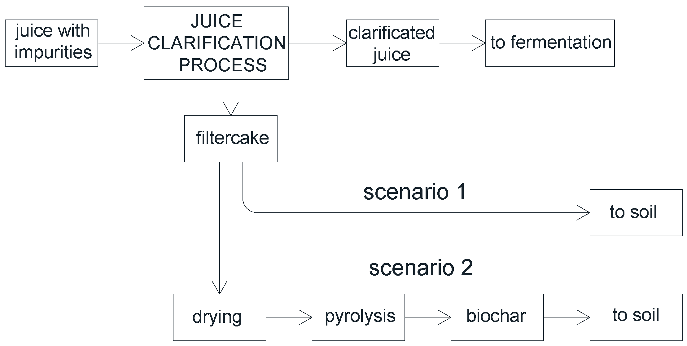
• Scenario 1, without the use of biochar, as shown in Equation (11);
• Scenario 2, with the use of biochar, as shown in Equation (12).

$$\sum {\epsilon }_{\left(1\right)}=\left({\epsilon }_{13\left(1\right)}+{\epsilon }_{14\left(1\right)}+{\epsilon }_{15\left(1\right)}+{\epsilon }_{16\left(1\right)}+\dots +{\epsilon }_{27\left(1\right)}+{\epsilon }_{28\left(1\right)}+{\epsilon }_{29\left(1\right)}+{\epsilon }_{30\left(1\right)}\right)$$

(11)

$$\sum {\epsilon }_{\left(2\right)}=({\epsilon }_{13\left(2\right)}+{\epsilon }_{14\left(2\right)}+{\epsilon }_{15\left(2\right)}+{\epsilon }_{16\left(2\right)}+\dots +{\epsilon }_{27\left(2\right)}+{\epsilon }_{28\left(2\right)}+{\epsilon }_{29\left(2\right)}+{\epsilon }_{30\left(2\right)})$$

(12)

CEENE initially accounted for each ton of cane produced, then the productivity of sugarcane for each hectare planted was considered, and finally, the productivity of ethanol was considered, which resulted in the irreversibilities in megajoules per megajoule of ethanol produced (MJ/MJ ethanol), as shown in Equation (13).

$$\mathrm{CEENE}=\frac{\mathrm{MJ}}{\mathrm{MJ}\mathrm{ethanol}}=\frac{\left(\frac{\mathrm{MJ}}{\mathrm{TC}}\right)\left(\mathrm{Prod}\_\mathrm{cane}\right)}{\left(\mathrm{Prod}\_\mathrm{ethanol}\right)\left({\mathrm{Ex}}_{\mathrm{ethanol}}\right)}$$

(13)

where CEENE: Cumulative Exergy Extraction from the Natural Environment per megajoule of ethanol produced (MJ/MJ); Prod_cane: productivity of sugarcane in tons of sugarcane per hectare (Mg/ha); Prod_ethanol: ethanol productivity per hectare (kg/ha); and Ex_ethanol: exergy of hydrated ethanol (MJ/kg)

As in the above-mentioned case of the emissions of nitrogen fertilization (ε₁₅) in Equation (10), we also individually calculated the exergy consumed (Ex₁₅) during the use of nitrogen fertilizer, initially per ton of sugarcane, as in Equation (14), and then, we transported this value to Equation (13). This item, as well as several other ones, has the characteristic of needing to add the energy consumed in the production of compost to the chemical exergy of compost because these two resources are being degraded.

$$Ex\left(15\right)=m_{\mathrm{N}/\mathrm{SCT}}{E}_N+m_{\mathrm{N}/\mathrm{TC}}{X}_N$$

(14)

where m_N/_SCT: nitrogen fertilizer mass per sugarcane ton (kg/SCT); EN: exergy consumed in the production of nitrogen fertilizer (MJ/kg); and X_N: chemical exergy of nitrogen fertilizer (MJ/kg).

Being an exergy input, the exergy of the sun (Ex₁), whose value must also be transferred to Equation (13), shall be calculated as shown in Equation (15).

$$X_{sun}=\left(10,000\right)\left(365\right)\left(0.9\right)\left(AR\right)$$

(15)

where Xsun: absorbed solar exergy per hectare in the cycle of one year (MJ/ha); 10,000 m² = 1 ha; 365 days a year; AR: average annual radiation for one day in the southeast region of Brazil (16 MJ/m² day); and “0.9”: exergy quality factor for sunlight.

In accordance with Equations (16) and (17) and inserting data from the exergy values in Table 2, the total extraction of exergy of the system was calculated for both scenarios, where this extraction (irreversibilities) is in megajoule units per kilogram of ethanol.

$${\mathrm{CEENE}}_1=\frac{{[(E{x}_5+E{x}_{10}+E{x}_{11}+E{x}_{12})-\left(E{x}_1+E{x}_2+E{x}_3+E{x}_{13}+\dots +E{x}_{29}\right)]}_1}{{\left(\mathrm{ethanol}\mathrm{mass}\right)}_1\left({\mathrm{Ex}}_{\mathrm{ethanol}}\right)}$$

(16)

$${\mathrm{CEENE}}_2=\frac{{[(E{x}_5+E{x}_{10}+E{x}_{11}+E{x}_{12})-\left(E{x}_1+E{x}_2+E{x}_3+E{x}_{13}+\dots +E{x}_{29}\right)]}_2}{{\left(\mathrm{ethanol}\mathrm{mass}\right)}_2\left({\mathrm{Ex}}_{\mathrm{ethanol}}\right)}$$

(17)

3. Results

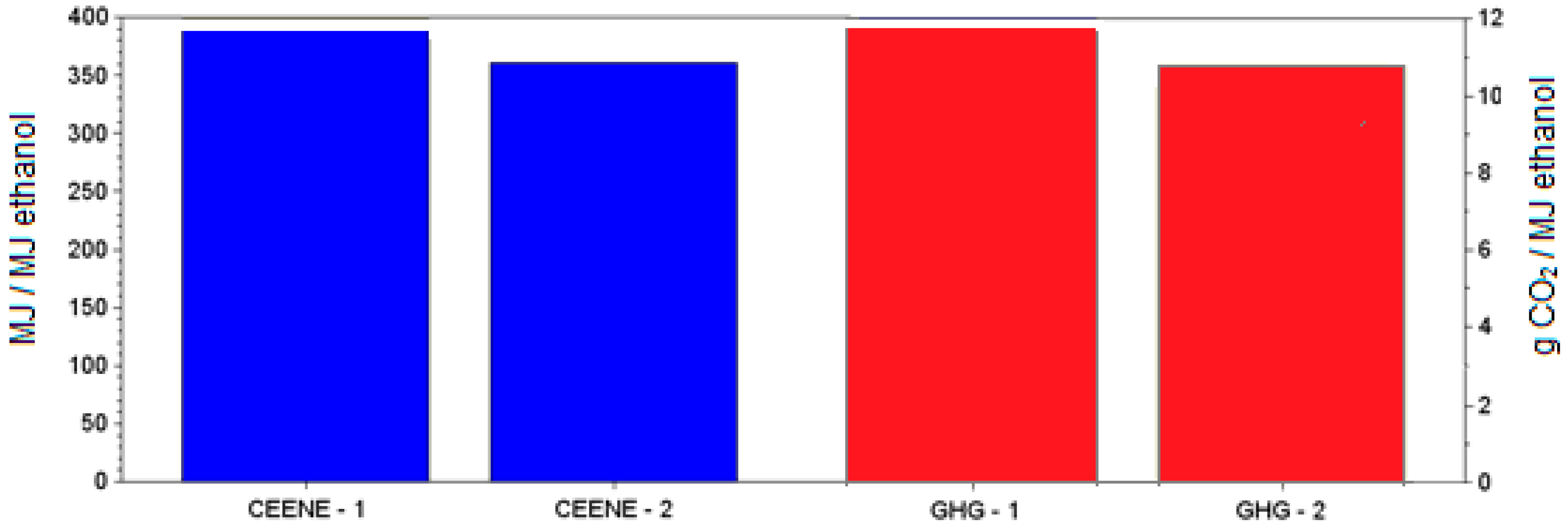
3.1. The Biochar Changing Scenarios

With the use of biochar, both the productivity of sugarcane and the nitrous oxide are altered, and the impacts of these variations are initially analyzed punctually and, later, more generally, when the same variables are scanned.

Figure 5 presents the exergy (CEENE) and GHG emissions behavior of scenarios 1 and 2. Exergy is calculated according to Equations (16) and (17), in MJ/MJ ethanol, and GHG emissions, in g CO_2-equivalent/MJ ethanol, is calculated according to Equations (11) and (12). The increase in productivity had the greatest contribution to the decrease of exergy extraction, and the influence of the nitrous oxide emissions is much less significant. In addition to the two causes are GHG emissions due to increased productivity and lower emissions of nitrous oxide itself, where increased productivity is more sensitive.

Figure 6 represents the values alteration concerning exergy–emissions rates for scenarios 1 and 2, according to Equation (6), in MJ/g CO_2-equivalent. It is observed that the exergy–emissions relationship remained relatively constant due to the simultaneous occurrence of increased productivity and the decrease in the nitrous oxide emissions with the use of biochar.

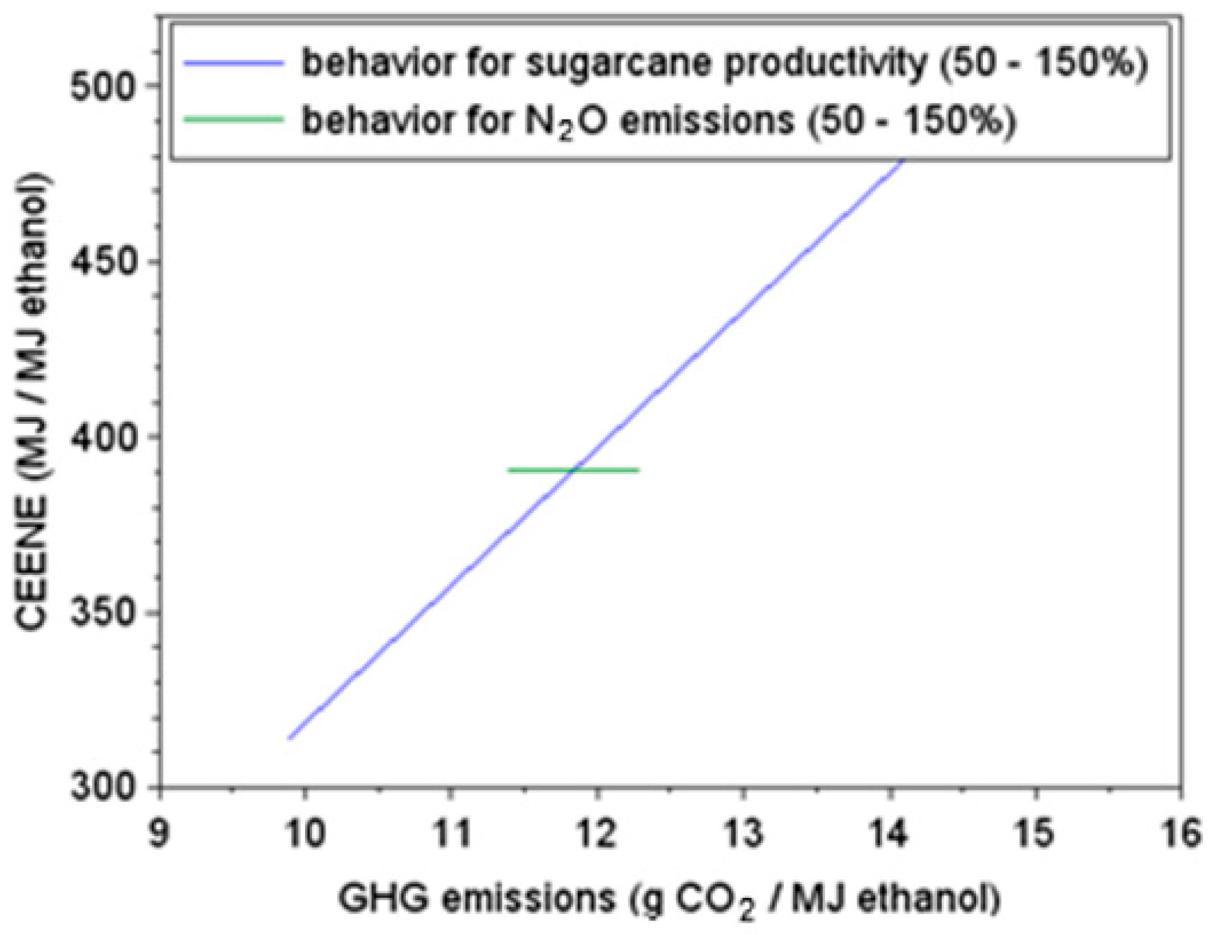
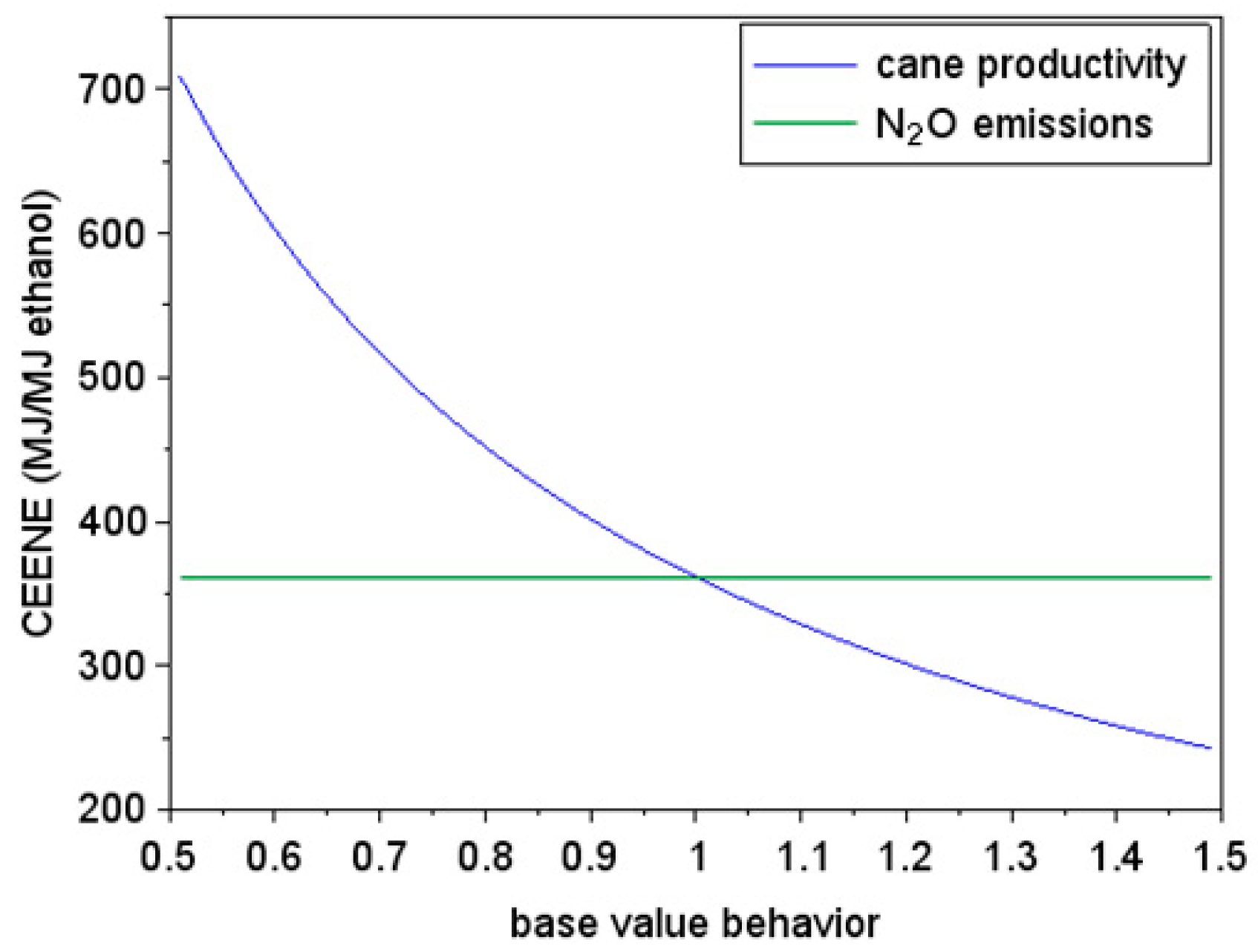
3.2. Scanning Production and N₂O Emissions

From the inventory database inserted in the Scilab numerical software, Figure 7 presents individually, through two functions, the relationship between CEENE and GHG emissions quantities. In the first function, the productivity of sugarcane varied between 50 and 150% (the other values are the same as those in RS, the reference system). The second function had the same percentages when varying the emissions of nitrous oxide. This figure shows a great sensitivity of CEENE and GHG emissions due to the sweep of productivity and the almost null sensitivity in the sweeping of nitrous oxide emissions in soil.

Using the algorithm in the Scilab numerical programming software, Equations (6), (11) and (16) are applied in an amplified way, when scanning from 50% to 150% around the base value, which is the reference value (X-axis). For example, for sugarcane productivity (Prod_cane), as shown in Equations (9) and (13), this value is 70 tons per hectare, i.e., scanning takes place from 35 and 105 tonnes per hectare, impacting (or not) on the outcomes of the Equation. The notable function behavior around the base value represents a greater or lesser sensitivity of the input.

3.2.1. The CEENE Behavior

Figure 8 presents the irreversibility values (CEENE), ranging from 50% to 150%, by inputs or products: (a) sugarcane productivity; (b) nitrous oxide emissions. In this figure, it is possible to observe the great sensitivity of the sugarcane productivity, calculated from the base value through Equation (8), at −0.49 and close to zero for the nitrous oxide emissions.

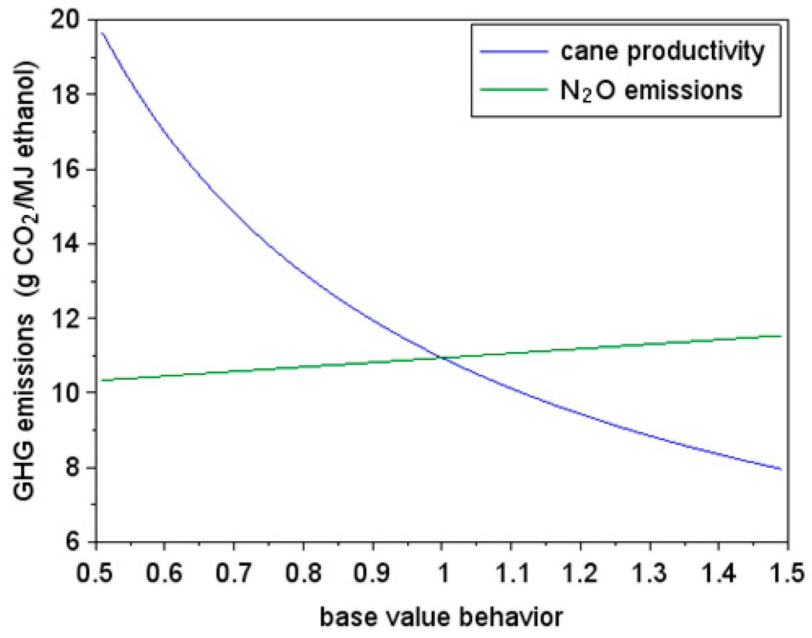
3.2.2. The GHG Behavior

Figure 9 presents the values of GHG emissions “ε” and the variables between 50% and 150% for the inputs or products: (a) sugarcane productivity; and (b) nitrous oxide emissions. The sensitivity of cane productivity from the base value is higher, according to Equation (8), at −0.41, and the nitrous oxide emissions are smaller, at 0.07.

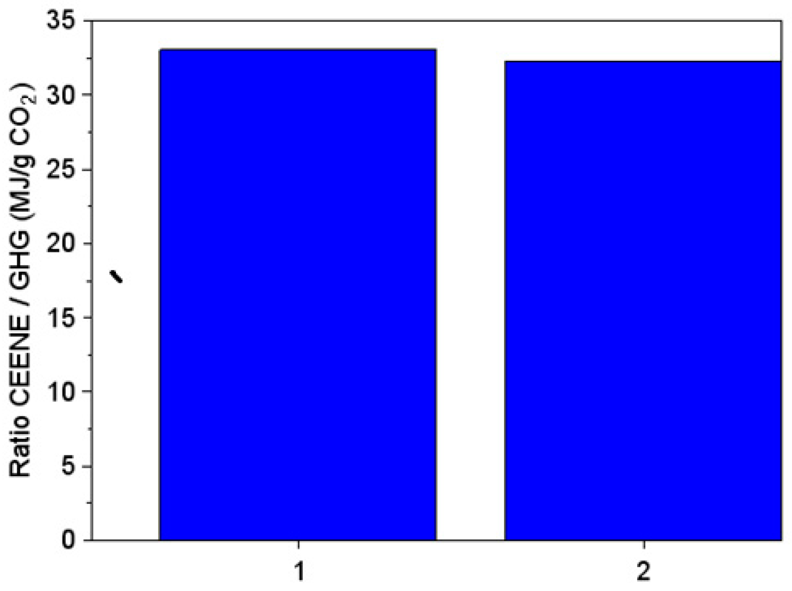
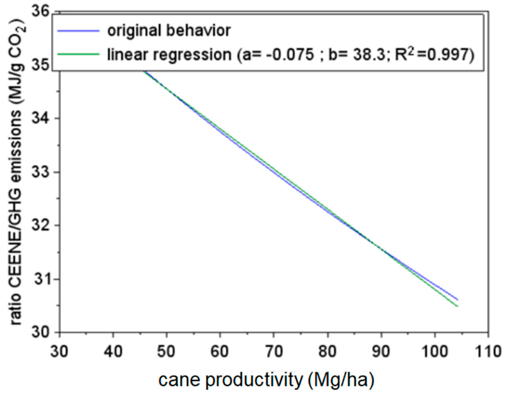
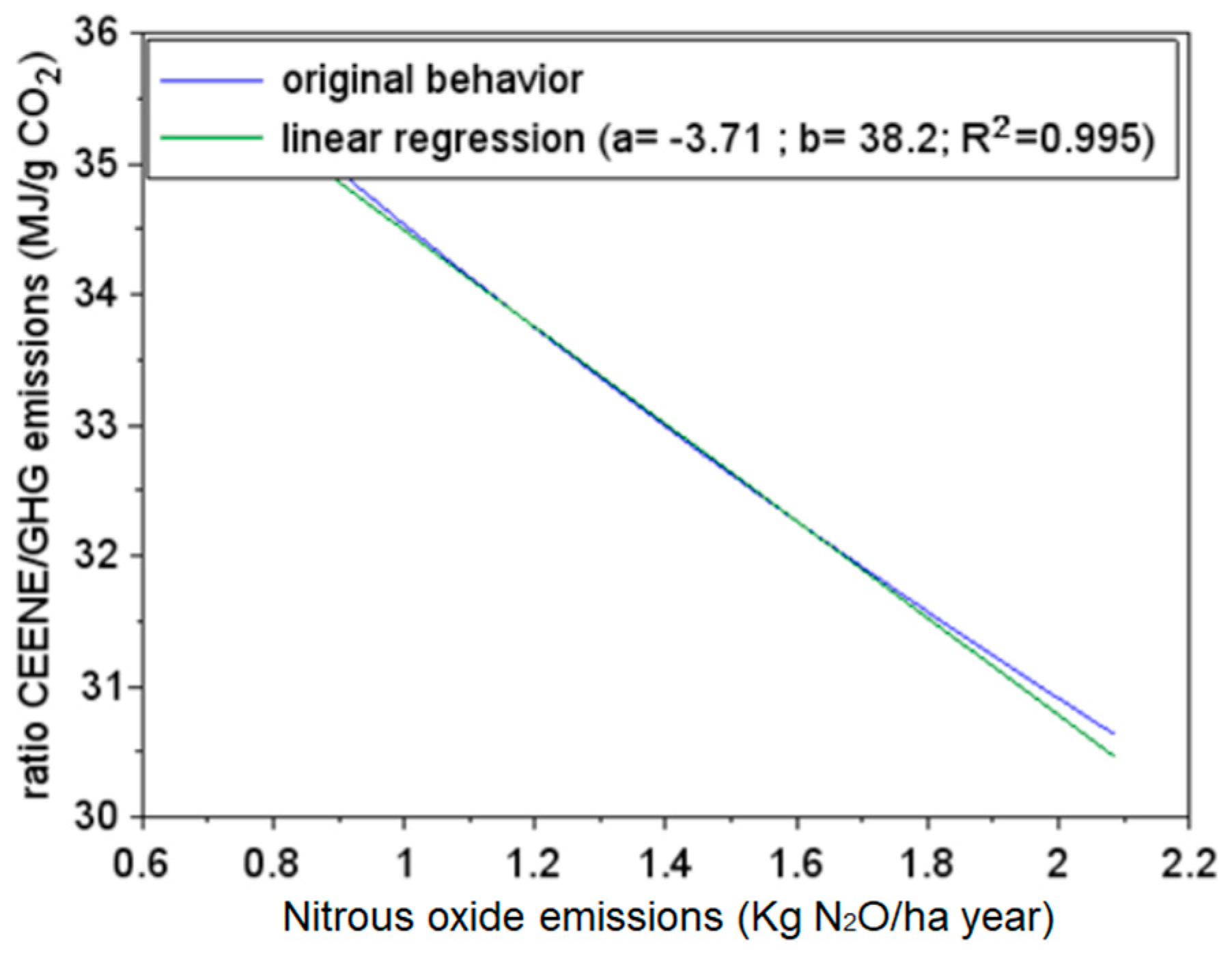
3.2.3. The Behavior ratio of CEENE: GHG and the Linear Function Result

The alterations of the ratio CEENE: emissions have been treated individually using Scilab numerical programming. The original vector and linear Y function (X₁) are presented, in Figure 10, in the same way as the original vector and linear Y function (X₂) were presented in Figure 11, and X₁ for sugarcane productivity and X₂ for nitrous oxide emissions are also presented. These functions presented a fairly linear behavior, which made it possible to represent them with a linear function.

A linear function simply represents the vector outcomes from which they originated. A simple linear regression (RLS), a and b values as well as the standard deviation were addressed with the reglin command [a, b, sig], where mean(Y(X_i)), representing the average and the coefficient of determination (R²), which were also calculated using Scilab. Equation (18), whose outcomes are presented in Figure 10 and Equation (19), is shown in Figure 11. After completing such equations, the aforementioned statistical data are also presented.

$$Y(X_1)=\left(-0.075\right)X_1+38.3$$

(18)

Average = 33.1

Coefficient of determination R² = 0.997

where $Y(X_1)$: the function that relates the exergy extraction with GHG emissions in accordance with productivity of sugarcane (MJ/g CO_2-equivalent); and X₁: productivity of sugarcane (SCT/ha).

$$Y(X_2)=\left(-3.71\right)X_2+38.3$$

(19)

Average = 33.1

Coefficient of determination R² = 0.995

where $Y(X_2)$: the function that relates the CEENE with GHG emissions on the basis of nitrous oxide emissions (MJ/g CO_2-equivalent); and X₂: variable nitrous oxide emissions (kg N₂O/ha year).

4. Discussion

Even at a very high value, the exergy of the sun is accounted for, being the great input of exergy in the system. The magnitude of this value results in large irreversibilities in the system, but CEENE’s behavior is proportional to this input since the emission values are independent of the greater or lesser radiation considered, which makes the CEENE: emissions ratio also proportional. As for the sensitivities, their magnitudes are not altered, but the behavior of the other variables that depend on the solar radiation, whose values are also proportional, is just as important.

As for the behavior shown in Figure 10 and Figure 11, it is important to note that all the variation occurs around the reference value of 33.1 MJ/g CO_2-equivalent, which is Y’s value at the center of the X axis. The variables that represent the productivity and emissions of N₂O, when undergoing changes due to the use of biochar, were specifically considered in these graphs. To a greater or lesser extent, the following variables were sensitive to the decrease of the value of Yi with the increase of Xi: ethanol productivity; the production of electricity; diesel transport/field; and the CO₂ generated in the fermentation and yield of sugar cane. In nitrogen fertilization and nitrous oxide emissions, the values of Yi remained practically constant.

For each megajoule of ethanol produced, the increase in productivity had a greater influence on the decrease in the exergy extraction, compared to the decrease in emissions, and Figure 10 presents this relation, which results in better use of resources when increasing productivity.

As for the irreversibilities in the numerator of Equation (7) and the emissions in the denominator, it should be noted that smaller values of this ratio are not necessarily indicative of a smaller number of irreversibilities generated, since the increase in the denominator also gives this result. From this, it can be understood that: the improvement of the system, with regard to the aspect of the efficient use of resources, depends on whether variable Xi is related to exergy or the emissions. An increase in the variable Xi, which represents nitrous oxide and ammonia, leads to apparently controversial results since they cause the decrease of the Y value. Due to the numerator of the Equation, the exergy consumption remains practically constant during the sweep from 50%–150% in X due to its low contribution to the exergy impacts.

The Y function presented in Figure 10 and Figure 11 depends on the exergy in the numerator and the emissions in the denominator, as already mentioned. The Equations presented already coupled these quantities as a function of X₁ and X₂.

The representation of the best use of carbon in the Y function may be the effect of the decrease in the value of its numerator (exergy) and denominator (emissions). Thus, more nitrous oxide represents a poor use of carbon, as well as a low productivity of sugarcane. Then, from Figure 10, the best use of carbon occurs with increasing productivity and, from Figure 11, with decreasing N₂O emissions.

As previously shown in Figure 9, the emissions value is already in grams of CO_2-equivalent per megajoules of ethanol, and this already represents the efficient use of carbon. Figure 10 and Figure 11 indicate that, from a base value of the reference system, the efficiency increased with the increase of X₁ or decrease of X₂.

5. Conclusions

In addition to presenting biochar as an industrial waste that has positive results when returned to the soil, with an increased productivity and reduction of nitrous oxide emissions in the soil, this study showed that, using the system, it is possible to perform a coupling between CEENE (cumulative exergy extraction from the natural environment) and air pollution in the form of greenhouse gases, where the ratio of these quantities is represented by the Y function. In the reference system (RS), the exergy:emissions ratio was calculated, with a value of 33.1 MJ/g CO_2-equivalent, which is changed as the variables present in the system under study are changed. By performing the irreversibility coupling, in the form of CEENE, with GHG emissions, initially through a function Y (X₁) and later Y (X₂), where X₁ represents the productivity and X₂, the emissions of nitrous oxide, the behavior of this ratio was almost linear, making it possible, through linear regression, to write an equation in the form, ax + b, which produced a = −0.075, b = 38.3 and R² = 0.997 for productivity (Mg SCT/ha year) and a = −3.71, b = 38.2 and R² = 0.995 for nitrous oxide emissions (kg N₂O/ha year).

In order to advise as to the better use of carbon, it is not necessary to calculate the CEENE: emissions ratio, since emissions are already accounted for in grams of CO_2-equivalent per megajoule of ethanol produced, where, in the graph dealing with the emissions behavior from the scans of sugarcane productivity and N₂O emissions in the soil, it is quite clear that less carbon is released into the atmosphere for each megajoule of ethanol produced by increasing productivity and decreasing N₂O emissions.

However, with some considerations, it is possible, through the equations that have been made, to achieve the same result using CEENE–emissions coupling. As a general rule, it can be said that, during the scanning of variables with greater sensitivity in the numerator of the Y function, lower values of Y indicate a better use of the carbon, and already for variables with a greater sensitivity in the denominator of the said function, lower values of Y indicate a worse use of carbon. In other words, the question is whether the variable under study is more sensitive to CENNE or emissions. For cane productivity, the CEENE sensitivity is 20% higher than the emissions (CEENE predominates, −0.49 versus −0.41). For emissions, it is almost zero, and for CEENE and emissions, it is 0.077, which predominates.

Thus, in a bioenergetic system, it was possible to correlate different metrics when making a coupling between the CEENE and the GHG emissions, whose ratio in the reference system was 33.1 MJ/g CO_2-equivalent. Besides relating these quantities, this ratio, to a greater or lesser extent, is altered both by the change in the exergy extraction and by the GHG emissions in the system, or even by both simultaneously, and when properly considered, this can indicate how carbon can be used more efficiently by the system under study.

References

1. BP Energy Outlook—2017 Edition. Available online: http://www.bp.com/energyoutlook#BPstats (accessed on 8 March 2018).
2. Graedel, T.E.; Allenby, B.R. Industrial Ecology: Policy Framework and Implementation, 2nd ed.; Prentice Hall: Englewood Cliffs, NJ, USA, 1999. [Google Scholar]
3. Kotas, T.J. Basic exergy concepts. In The Exergy Method of Termal Plant Analysis; Reprint Edition; Krienger Publishing Company: Malabar, FL, USA, 1995; pp. 29–56. [Google Scholar]
4. Sciubba, E.; Wall, G. A brief Commented History of Exergy from the Beginnings to 2004. Int. J. Chem. Thermodyn. 2007, 10, 1–26. [Google Scholar]
5. Wall, G. Exergy and resource accounting. In Exergy—A Useful Concept within Resource Accounting; Institute of Theoretical Physics, Chalmers University of Technology and University of Göteborg: Göteborg, Sweden, 1977; pp. 15–36. [Google Scholar]
6. Rifkin, J.; Howard, T. Entropy into the Greenhouse World; Revised Edition; New Age Book: New York, NY, USA, 1990. [Google Scholar]
7. Cornelissen, R.L. Thermodynamics and Sustainable Development. Ph.D. Thesis, University of Twente, Enschede, The Netherlands, 1997. [Google Scholar]
8. Szargut, J.; Morris, D.R. Cumulative Exergy Consumption and Cumulative Degree of Perfection. In Exergy Analysis of Thermal, Chemical and Metallurgical Processes, 1st ed.; Hemisphere Publishing: New York, NY, USA, 1988; pp. 171–191. [Google Scholar]
9. Dewulf, J.; Bösch, M.E.; De Meester, B.; Van Der Vorst, G.; Van Langenhove, H.; Hellweg, S.; Huijbregts, M.A.J. Cumulative exergy extraction from the natural environment (CEENE): A comprehensive life cycle impact assessment method for resource accounting. Environ. Sci. Technol. 2007, 41, 8477–8483. [Google Scholar] [CrossRef] [PubMed]
10. Mcmanus, M.C.; Taylor, C.M. The changing nature of life cycle assessment. Biomass Bioenergy 2015, 82, 13–26. [Google Scholar] [CrossRef] [PubMed] [Green Version]
11. Macedo, I.C.; Leal, M.R.L.V.; Silva, J.E.A.R. Balanço das emissões de gases do efeito estufa na produção e no uso do etanol no Brasil; Núcleo Interdisciplinar de Planejamento Energético da Universidade Estadual de Campinas–NIPE/UNICAMP: Campinas, SP, Brasil, 2004; pp. 9–37. [Google Scholar]
12. Szargut, J. Calculation of exergy. In Exergy Method—Tecnical and Ecological Applications, 1st ed.; WIT Press: Southampton, UK, 2005; pp. 19–54. [Google Scholar]
13. Hoang, V.N.; Rao, D.S.P. Measuring and decomposing sustainable efficiency in agricultural production: A cumulative exergy balance approach. Ecol. Econ. Mag. 2010, 69, 1765–1776. [Google Scholar] [CrossRef]
14. Maes, D.; Passel, S.V. Advantages and limitations of exergy indicators to assess sustainability of bioenergy and biobased materials. Environ. Impact Assess. Rev. 2014, 45, 19–29. [Google Scholar] [CrossRef] [Green Version]
15. Hovelius, K.; Wall, G. Energy, exergy and emergy analysis of a renewable energy system based on biomass production. In Proceedings of the Efficiency, Costs, Optimization, Simulation and Environmental Aspects of Energy Systems, ECOS’98, Nancy, France, 8–10 July 1998; pp. 1197–1204, ISBN 2-905-267-29-1. [Google Scholar]
16. Saltelli, A.; Ratto, M.; Andres, T.; Campolongo, F.; Cariboni, J.; Gatelli, D.; Saisana, M.; Tarantola, S. Elementary Effects Method. In Global Sensitivity Analysis; John Wiley & Sons Ltd.: Chichester, UK, 2008; pp. 109–131. [Google Scholar]
17. Hamby, D.M. A review of techniques for parameter sensitivity analysis of environmental models. Environ. Monit. Assess. 1994, 32, 135–154. [Google Scholar] [CrossRef] [PubMed] [Green Version]
18. Scilab (Version 6.0.1). Available online: http://www.scilab.org/download/6.0.1 (accessed on 4 June 2018).
19. Macedo, I.C.; Seabra, J.E.A.; Silva, J.E.A.R. Green house gases emissions in the production and use of ethanol from sugarcane in Brazil: The 2005/2006 averages and a prediction for 2020. Biomass Bioenergy 2008, 32, 582–595. [Google Scholar] [CrossRef]
20. ANP (Agência Nacional de Petróleo). Available online: www.anp.gov.br/?dw=82253 (accessed on 17 October 2018).
21. Dirbeba, M.J.; Brink, A.; Demartini, N.; Zevenhoven, M.; Hupa, M. Potential for thermochemical conversion of biomass residues from the integrated sugar-ethanol process: Fate of ash and ash-forming elements. Bioresour. Technol. 2017, 234, 188–197. [Google Scholar] [CrossRef] [PubMed]
22. Kamate, S.; Gangavati, P. Exergy analysis of cogeneration power plants in sugar industries. Appl. Therm. Eng. 2009, 29, 1187–1194. [Google Scholar] [CrossRef]
23. Santos, N.A.V.; Vieira, S.S.; Mendonça, F.G.; Napolitano, M.N.; Nunes, D.M.; Ferreira, R.A.R.; Soares, R.R.; Magriotis, Z.M.; Araujo, M.H.; Lago, R.M. Rejeitos de Biomassas Oriundas da Cadeia de Biocombustíveis no Brasil: Produção de Bio-óleo e Sub-produtos. Rev. Virt. Quím. 2017, 9, 1–21. [Google Scholar]
24. Palacios-Bereche, R.; Mosqueira-Salazar, K.J.; Modesto, M.; Ensinas, V.A. Exergetic analysis of the integrated first and second-genaration etanol production from sugarcane. Energy 2013, 62, 46–61. [Google Scholar] [CrossRef]
25. Zhang, H.; Xiao, R.; Jin, B.; Shen, D.; Chen, R.; Xiao, G. Catalytic fast pyrolysis of straw biomass in an internally interconnected fluidized bed to produce aromatics and olefins: Effect of different catalysts. Bioresour. Technol. 2013, 137, 82. [Google Scholar] [CrossRef] [PubMed]
26. NOVACANA. Available online: https://www.novacana.com/cana/glossario-de-indicadores-de-pd-na-cadeia-produtiva-cana-etanol (accessed on 27 November 2018).
27. INPE (Atlas Brasileiro de Energia Solar, 2006). Available online: ftp.cptec.inpe.br/labren/publ/livros/brazil_solar_atlas_R1.pdf (accessed on 2 November 2017).
28. Jeffery, S.; Verheijen, F.G.A.; Velde, M.; Bastos, A.C. A quantitative review of the effects of biochar application to soils on crop productivity using meta-analysis. Agric. Ecosyst. Environ. 2011, 144, 175–187. [Google Scholar] [CrossRef]
29. Cayuelaa, M.L.; van Zwietenb, L.; Singhb, B.P.; Jefferyc, S.; Roiga, A.; Sánchez-Monedero, M.A. Biochar’s role in mitigating soil nitrous oxide emissions: A review and meta-analysis. Agric. Ecosyst. Environ. 2014, 191, 5–16. [Google Scholar] [CrossRef]
30. IPCC - Fifth Assessment Report (AR5). Available online: /www.ipcc.ch/report/ar5/syr/2014 (accessed on 10 November 2017).
Figure 1. General flowchart of the process (mass and energy).
Energies 12 01057 g001
Figure 2. Capture and CO2-equivalent emissions in the sucroenergy sector (arrows represent proportionality values).
Energies 12 01057 g002
Figure 3. Exergy flows in the sucroenergy sector (arrows represent proportionality values, except that with the caption, “SUN”).
Energies 12 01057 g003
Figure 4. Obtention and destinations of the filtercake.
Energies 12 01057 g004
Figure 5. Greenhouse gases (GHG) and exergy alterations for both scenarios.
Energies 12 01057 g005
Figure 6. CEENE/GHG emissions relationship alterations for the scenarios.
Energies 12 01057 g006
Figure 7. Relationship of CEENE and GHG emissions with (a) the variation of sugarcane productivity; (b) the N2O variation emitted in the soil.
Energies 12 01057 g007
Figure 8. CEENE behavior of the variable cane productivity and N2O emissions (50%–150%).
Energies 12 01057 g008
Figure 9. GHG behavior of the variable cane productivity and N2O emissions (50%–150%).
Energies 12 01057 g009
Figure 10. Y function behavior for sugarcane productivity (50% to 150%).
Energies 12 01057 g010
Figure 11. Y function behavior for nitrogen fertilization (50% to 150%).
Energies 12 01057 g011