Article

Optimal Planning of Integrated Energy Systems for Offshore Oil Extraction and Processing Platforms

1
School of Electrical and Information Engineering, Southwest Petroleum University, Chengdu 610500, China
2
School of Engineering, Cardiff University, Cardiff CF24 3AA, UK
*
Author to whom correspondence should be addressed.
Energies 2019, 12(4), 756; https://doi.org/10.3390/en12040756
Submission received: 18 January 2019 / Revised: 20 February 2019 / Accepted: 21 February 2019 / Published: 24 February 2019
(This article belongs to the Section B: Energy and Environment)

Abstract

:
With the introduction of new technologies, such as waste heat recovery units (WHRU), associated gas utilization, the energy flow coupling relationship is further deepened within the energy system of the offshore oil and gas production platform. Besides, the energy system is closely linked with the oil and gas production system, and a closed-loop relationship between energy flow and material flow can be revealed. Uncertainties of energy supply and production process may lead to system-wide fluctuations, which threaten the stable operation of the platform. Therefore, an optimal planning model of integrated energy system for offshore oil and gas production platform is proposed in this paper. Firstly, a generalized energy and material flow model is proposed, three matrixes are defined based on laws of thermodynamics, including energy matrix, process matrix and feedback matrix. Secondly, the energy-material conversion relationship between the energy system and production system of a typical offshore oil and gas platform is quantitatively described, together with the coupling between the input and output of the two systems. Thirdly, considering the energy-material balance constraints and the uncertainties of production system, a multi-objective stochastic planning model for the offshore integrated energy system is established, which takes economics and environmental protection into consideration. A Monte Carlo simulation-based NSGA-II algorithm is proposed to solve the model. Finally, the validity and feasibility of the proposed methodology are demonstrated through an offshore oil and gas platform in Bohai, China. Compared with the traditional planning method, the total cost and CO2 emissions of the proposed method are reduced by 18.9% and 17.3%, respectively.

1. Introduction

Serious environmental challenges and a plummeting international oil price facing the market, have put the offshore oil industry in a dilemma: how to mitigate the CO2 emissions from offshore oil projects without increasing the capital expenditure significantly [1]. In Norway, about 62% of the carbon dioxide emissions in 2012 came from offshore oil extraction and processing tasks [2]. As a result, a lot of efforts have been put into developing energy efficient technologies to mitigate the CO2 emissions in offshore oil facilities. In general, the most feasible current ways to realize CO2 emission reduction in a cost effective way include: (i) improving the efficiency of energy generation and utilization, (ii) the use of offshore energy generation technologies [3].
The production system is a crucial part of offshore platforms and it is energy-intensive. Energy management is necessary to ensure the stability and safety of production system operations [4,5]. The fluids are extracted from wells and transported to the production system through manifolds. In the production system, oil, associated gas, and water in streams are separated and treated before being exported to the shore or released into the environment. Besides, the integrated energy system provides electrical power and heat required for operating the extraction, separation, and compression. Gas turbine generators and gas/oil fired boilers were employed as the electric and thermal energy sources, and the associated gases (AS) was used as fuel for the generators [6]. During oil production, the light hydrocarbons and other impurities dissolved or dispersed in the heavier hydrocarbon compounds (crude oil) are separated and released from well fluids under low-pressure conditions. This is called the associated gases. A flare gas recovery system (FGRS) is designed to minimize the amount of associated gas being flared either as a means of disposal or as a safety measure to relieve gas pressure. The methods used by FGRSs include gas collection, compression, electricity generation, and gas to liquid conversion, etc. For example, the associated gas can be injected to the existing gas distribution networks after exported from an offshore location, or it can be converted into electricity in offshore platforms and then transmitted to shore [7]. If the volume of associated gas with oil production is high enough, it can also be liquefied for sale [8,9]. Additionally, considering that approximately 50% of the total energy supplied to offshore oil and gas platforms is lost through exhaust flues, waste heat recovery units (WHRU) are employed to reuse the heat in the waste gas [10]. In [11], a supercritical carbon dioxide Brayton cycle was tested in a WHRU, and it performed better for energy-saving and emission mitigating than a simple Brayton cycle. In [12], a comparison between a single loop and a dual loop WHRU was conducted, and an organic Rankine cycle (ORC) was recommended to be added into the single loop WHRU to improve its efficiency. In addition, a multi-objective optimization method was proposed to select the working fluid of an ORC, considering efficiency, weight and space of an offshore platform, and the NSGA-II method was used to solve the optimization model [13]. A detailed mathematical optimization model for a WHRU based on ORC was presented to calculate the steady-state operational point of the WHRU, and the SQP solver was used to solve the model [14]. Design, sizing, and operating of the multiple components of such systems are generally challenging, especially when multiple conflicting objectives are aimed. Optimisation techniques based on meta-heuristics population approaches such as the Genetic Algorithm and Particle Swarm Optimisation were used to deal with these issues [15,16]. In general, the ORC was considered as a promising technology to utilize the medium-quality-heat sources with highest recovery efficiency in offshore oil industries [17,18]. Recently, carbon capture and storage (CCS) systems have been installed in offshore platforms for further mitigation of CO2 emissions. In [19], the Exergy balance of two platform configurations, with and without CCS, were assessed and the potential opportunities were found for improving the efficiency of the CCS section. In [1], a CCS with the pre-treatment and post-combustion units was proposed, which reduces the CO2 emissions of a platform in the North Sea by more than 15%. However, as a CCS itself is an energy-intensive unit, the introduction of a CCS reduces the CO2 emissions, it also causes the deterioration of the energy efficiency of offshore platforms [20].
It is noted that new technologies such as WHRU and ORC are not widely implemented in offshore oil extraction and processing platform, and the implementation of CO2-capture systems has not be proven offshore except for gas processing with high CO2-contents. To explore the feasibility of these new technologies in marine engineering, this paper introduce the various abovementioned technologies into the Bohai oil and gas platform to modify the structure of the offshore platform energy system. Simultaneously, there are significant discrepancies between the available energy and the power demands. Hence, it is necessary to coordinate the use of various energies, i.e., electrical power, heat, associated gas, and imported fuel (diesel in most methods). In this paper, the energy system of the offshore oil extraction and processing platform is regarded as an Integrated Energy System (IES) for considering the coupling of multiple forms of energy [21].
At present, many researchers have addressed the problem of the uncertainty planning of IES worldwide [22]. A bi-level fuzzy programming method was developed in [23] for energy systems planning and carbon dioxide mitigation under uncertainty, and the linear ranking function the first of Yager was used to solve the model. In [24], a bi-objective mathematical model was presented for energy hub scheduling with consideration of preventive maintenance policy to determine the preventive maintenance cycles and the best strategy to allocate hub energy capacity under different demand scenarios, and CPLEX Optimizer of the General Algebraic Modeling System (GAMS) was used to solve the model based on the Epsilon-constraint method. The concept of probabilistic power flow in power systems was extended to IES because of the coupling relationship between power systems, thermal systems and natural gas systems [25,26]. A chance constrained and reliability programming optimization model was proposed for solving the long-term integrated energy planning problem and their performances in [25], and then a chance constrained planning approach was proposed to minimize the investment cost of integrating new natural gas-fired generators, natural gas pipeline, compressors, and storage required to ensure desired confidence levels of meeting future stochastic power and natural gas demands in [26]. A two-stage stochastic multi-objective optimization algorithm was proposed to solve the optimal capacity of the cogeneration system under uncertain energy demand, the “greedy” approach was used to solve the problem in [27]. A robust optimization method incorporating piecewise linear thermal efficiency and electrical efficiency curves was proposed to deal with the uncertainties caused by energy supply, load prediction and equipment nonlinear efficiency, and a Monte Carlo simulation was adopted to sample random variables to demonstrate the effectiveness of the uncertain set in the robust optimization model in [28], and a two-interval mixed integer linear programming model and its solution algorithm were proposed for planning integrated energy-environment system in [29]. The uncertainties of energy supply, energy coupling, and load fluctuation have been considered in the mentioned papers. However, only energy systems are considered in most of studies, but the energy supply system is closely linked with the production system in offshore oil and gas production platform, and a closed-loop relationship between energy flow and material flow can be revealed. Due to the uncertainty of the production system is the most important factor for the offshore platform, it is essential to describe the relationship between energy supply system and production system, and explore the impact of this uncertainty on the planning of offshore platform energy supply systems, which are the innovations of this paper seldomly studied.
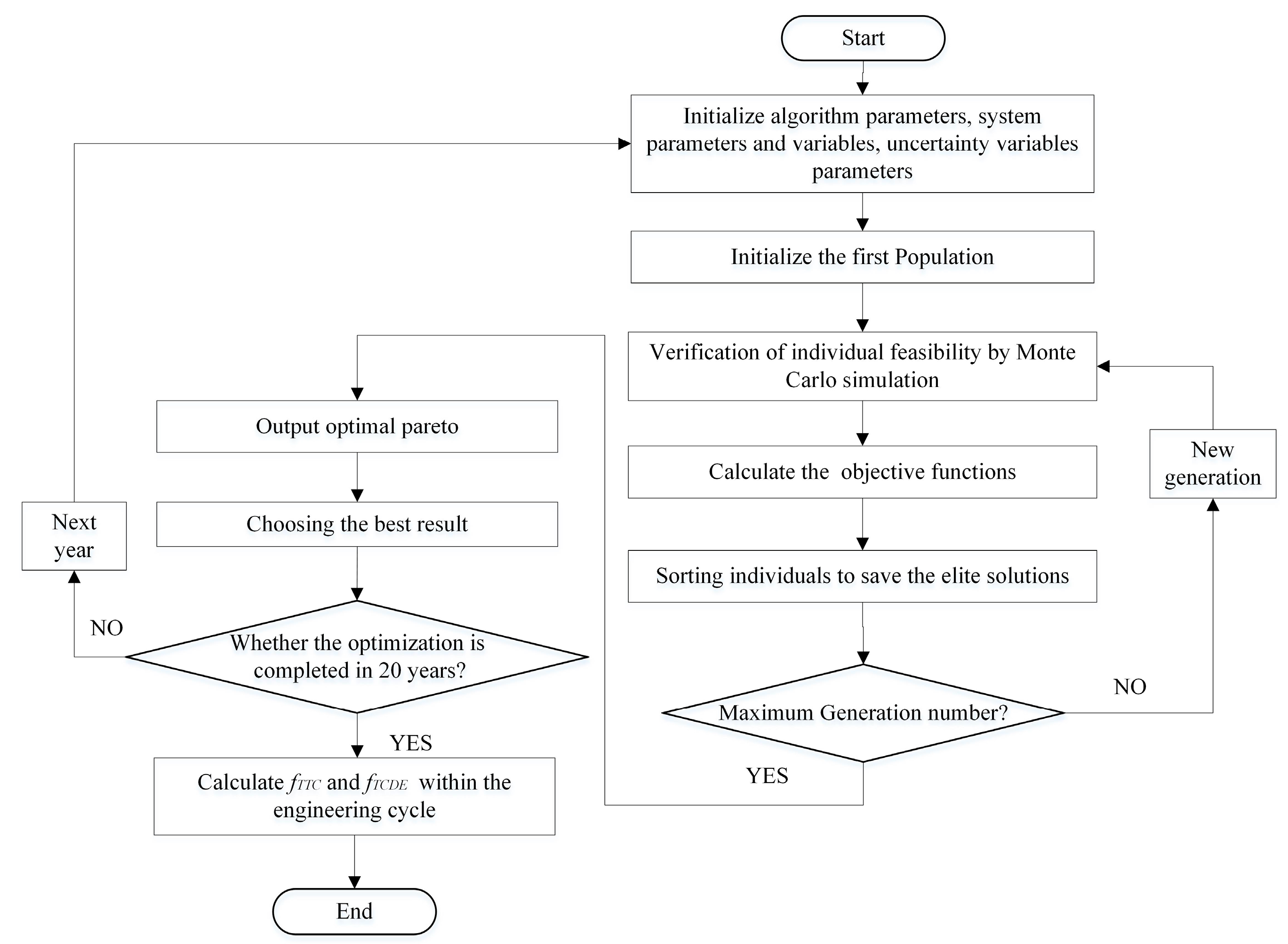
The main contributions of this paper are as follows: Firstly, based on the structural coupling features between IES and production system of offshore oil and gas platform, a generalized energy and material flow model is proposed, which describes the multi-energy coupling relationship and correlation between energy system and production system. The IES discussed in this paper includes multi-fuel gas turbines, waste heat boilers, ORC, CCS and power storage. Secondly, the energy-material flow and conversion relationship in production systems are quantitatively calculated based on enthalpy analysis. Thirdly, considering the energy-material balance constraints and the uncertainties of production system, a multi-objective stochastic planning model for the offshore IES is established, which takes economics and environmental protection into consideration. A Monte Carlo simulation based Non-dominated Sorting Genetic Algorithms II (NSGA-II) is proposed to solve the model. Finally, the validity and feasibility of the proposed methodology are demonstrated through an offshore oil and gas platform in Bohai, China.
This paper is organized as follows: the specific properties of the investigated system architecture and the proposed IES are described in Section 2, followed by a generalized energy and material flow model and its mapping details in Section 3. Section 4 presents the stochastic multi-objective optimization method to plan the IES for the offshore oil project, and Section 5 discusses the results of the optimization in detail. Concluding remarks are given in Section 6.

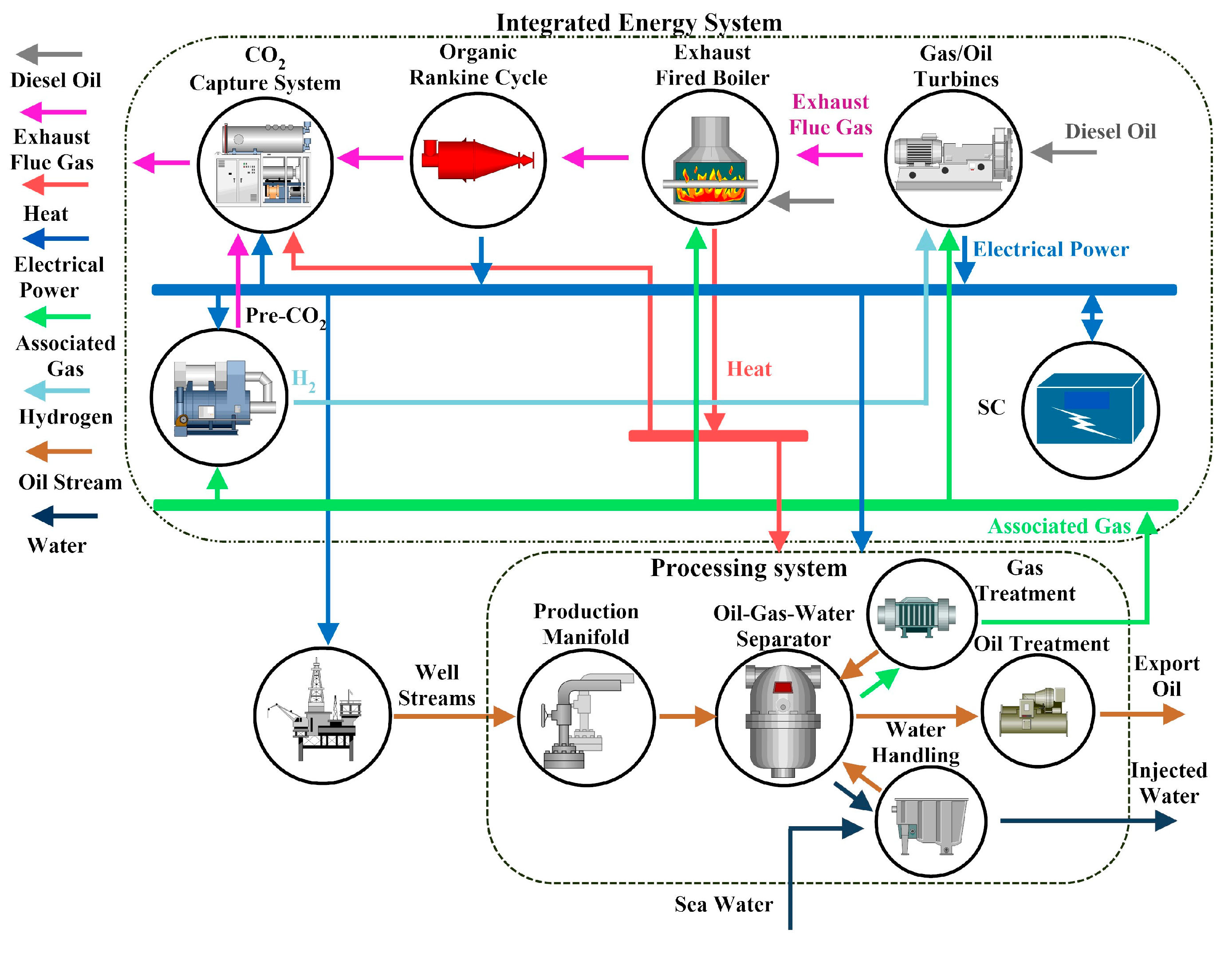
2. IESs for Offshore Oil Extraction and Processing

An existing offshore oil project, which consists of four offshore platforms, including one oil extraction and processing platform, one support and maintenance platform, one oil storage platform and one mooring platform is employed as a reference. The oil extraction and processing platform is also the central power platform which provides power for the other platforms through subsea cables. The platform facilities are characterized by a peak power demand of about 44 MW and a heating demand greater than 12 MW. The temperature range of heat loads is from 50 °C to 120 °C. Two turbines are used to generate power using diesel oil or gas. An exhaust fired boiler uses turbine exhaust with a temperature near 500 °C to heat oil and adjusts its combustion to ensure heat exchanger meet the load requirements. The thermal efficiency of the gas turbines varies from 27% to 32%. The total daily CO2 emissions produced reach about 300–500 tons, and more than 80% corresponds to the operation of gas turbines.
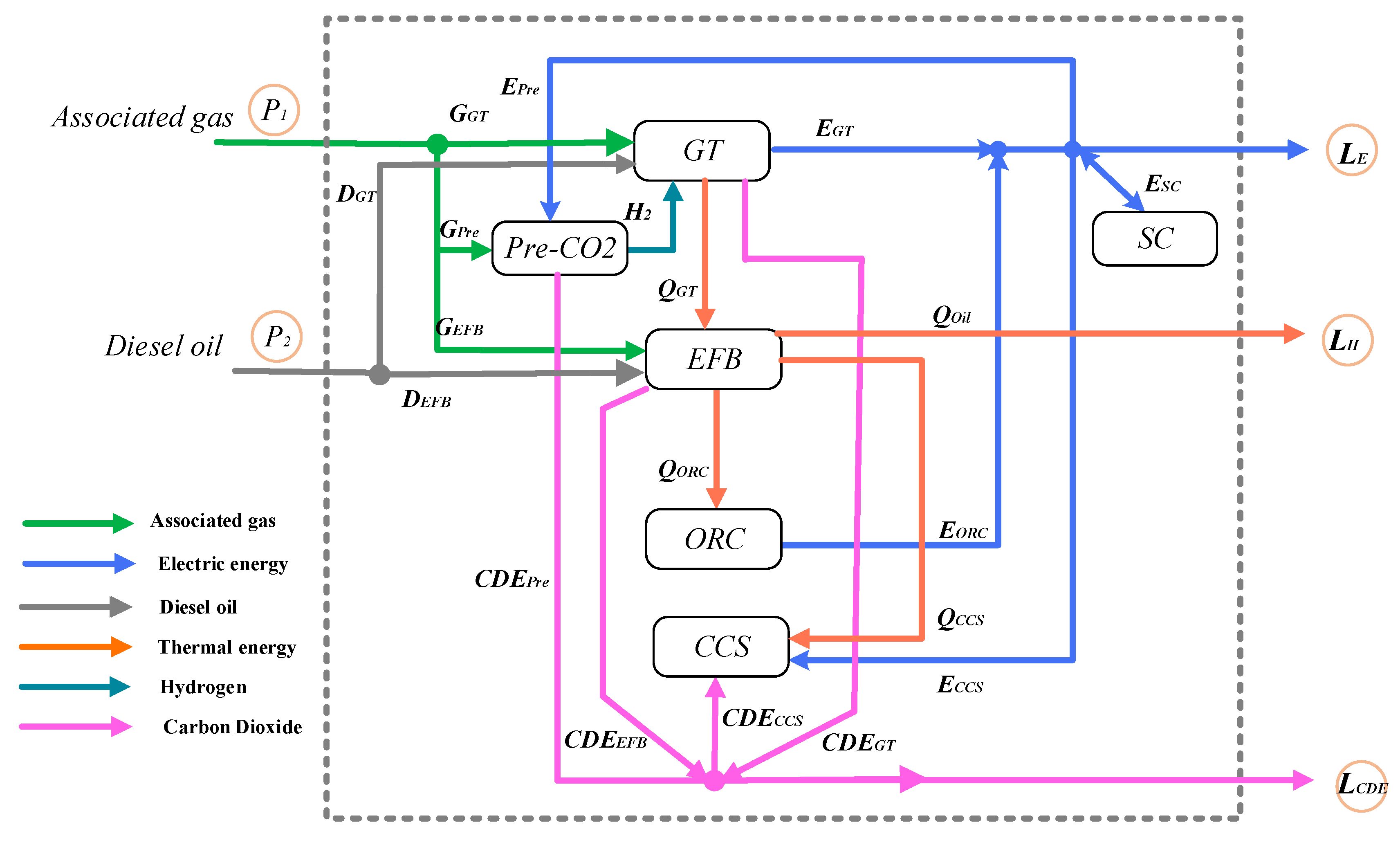
In this study, gas turbines are replaced by co-firing gas/oil turbines which can consume diesel, natural gas, and hydrogen. An ORC is employed to recover the exhaust heat of the boiler at about 160 °C–220 °C to improve the thermal efficiency further. Therefore, the ORC and the boiler constitute a heat recovery system of hierarchy, and the higher temperature (from 400 °C to 500 °C) and the lower temperature (from 160 °C to 220 °C) heat can be recovered simultaneously. Moreover, a two-level CO2 capture unit proposed in [1] for an oil platform is used to mitigate the emissions. The first level is a Pre-CO2 capture unit with the structure presented in [30], where natural gas is converted into hydrogen. The CO2 generated in the conversion is absorbed by chemical absorption with triethanolamine and the hydrogen is fed to the turbines. The second level is a Post-CO2 capture unit which is responsible for the carbon capture of the flue gas. A super-capacitor (SC) based energy storage is used to balance the source and loads. Figure 1 illustrates the proposed IESs and its relationship with the offshore oil extraction and processing system.

3. Generalized Energy and Material Flow Model

Different from multi-energy systems connected to electricity grids, the IESs for offshore oil platforms must run independently. They are sensitive to the fluctuations in extraction and processing systems. As a result, when a mathematic model is employed to describe such an IES shown in Figure 1, the impact of extraction and processing systems on the electricity and thermal consumption cannot be neglected. Moreover, material flows in addition to energy flows need to be considered in an IES. For example, the process in 
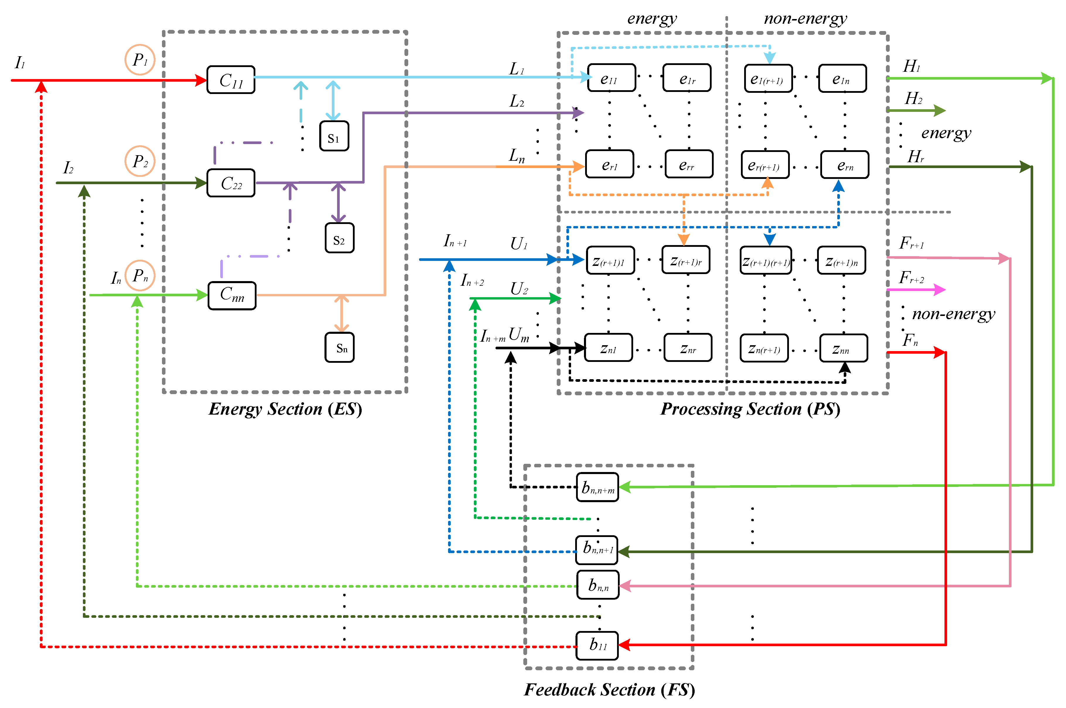
Figure 1 consumes the heat and electrical power generated from the IES and handles sea water and oil streams as well. At the same time, the processing system produces associated gas for the IES, which sends the energy to the processing system. Energy and material flow model of such a system can be represented by Figure 2.
In Figure 2, the Energy Section represents IESs, such as the one in Figure 1. Mathematically, the mapping of energies from the input to the output of the Energy Section can be described by an energy hub model, which provides the essential features of input and output, conversion, and storage of different energy carriers, shown as Equation (1) [31]:
[ L 1 L 2 L n ] L = [ c 11 c 12 c 1 m c 21 c 22 c 2 m c n 1 c n 2 c n m ] C [ P 1 P 2 P m ] P [ S 1 S 2 S n ] S , ( 0 c n m 1 )
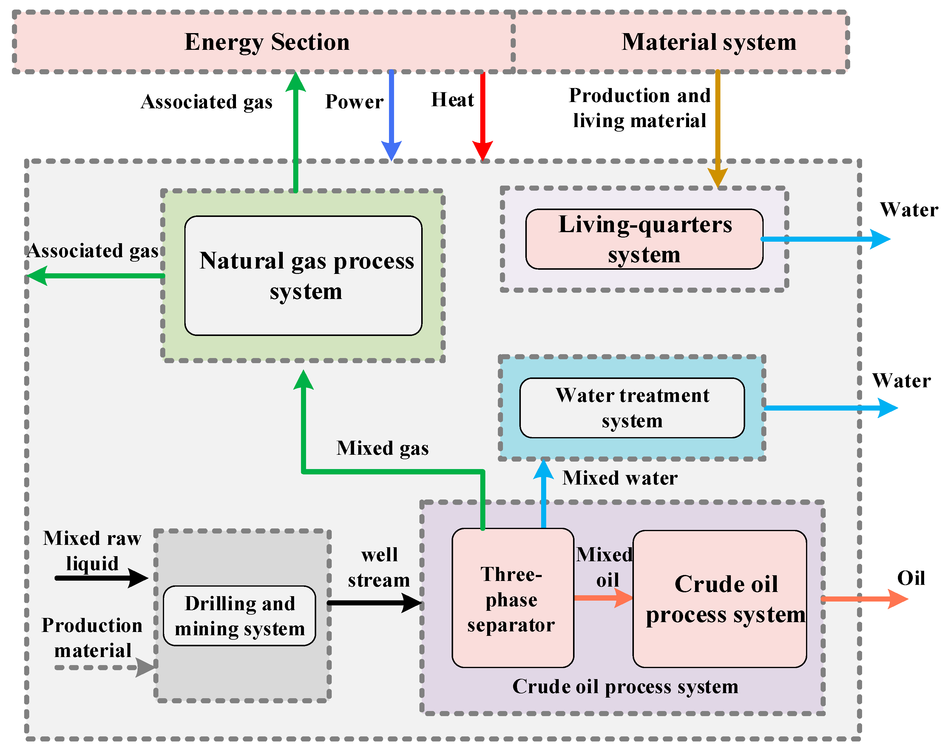
The Process Section denotes the process of production, e.g., the extraction and processing of oil, where the energies from Energy Section are consumed. Also, necessary materials used in the process are input into the Process Section, e.g., water and catalyst. In this section, a processing system can be divided into several sub-systems according to their functions, e.g., the Process Section in Figure 1 includes a drilling and mining system, a crude oil process system, a natural gas system, a water treatment system, and a living-quarters system. Based on energy and material (non-energy) consumption in Process Section, a multi-input and multi-output mapping is developed as shown in 
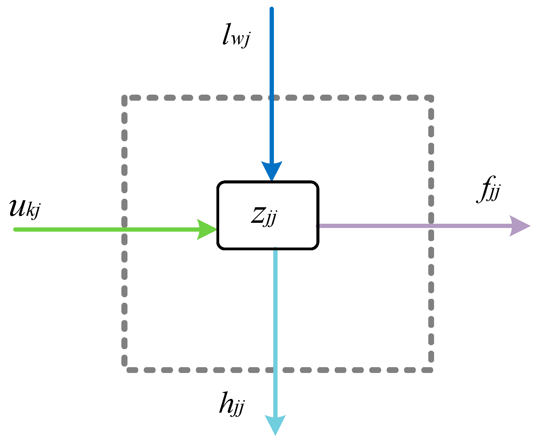
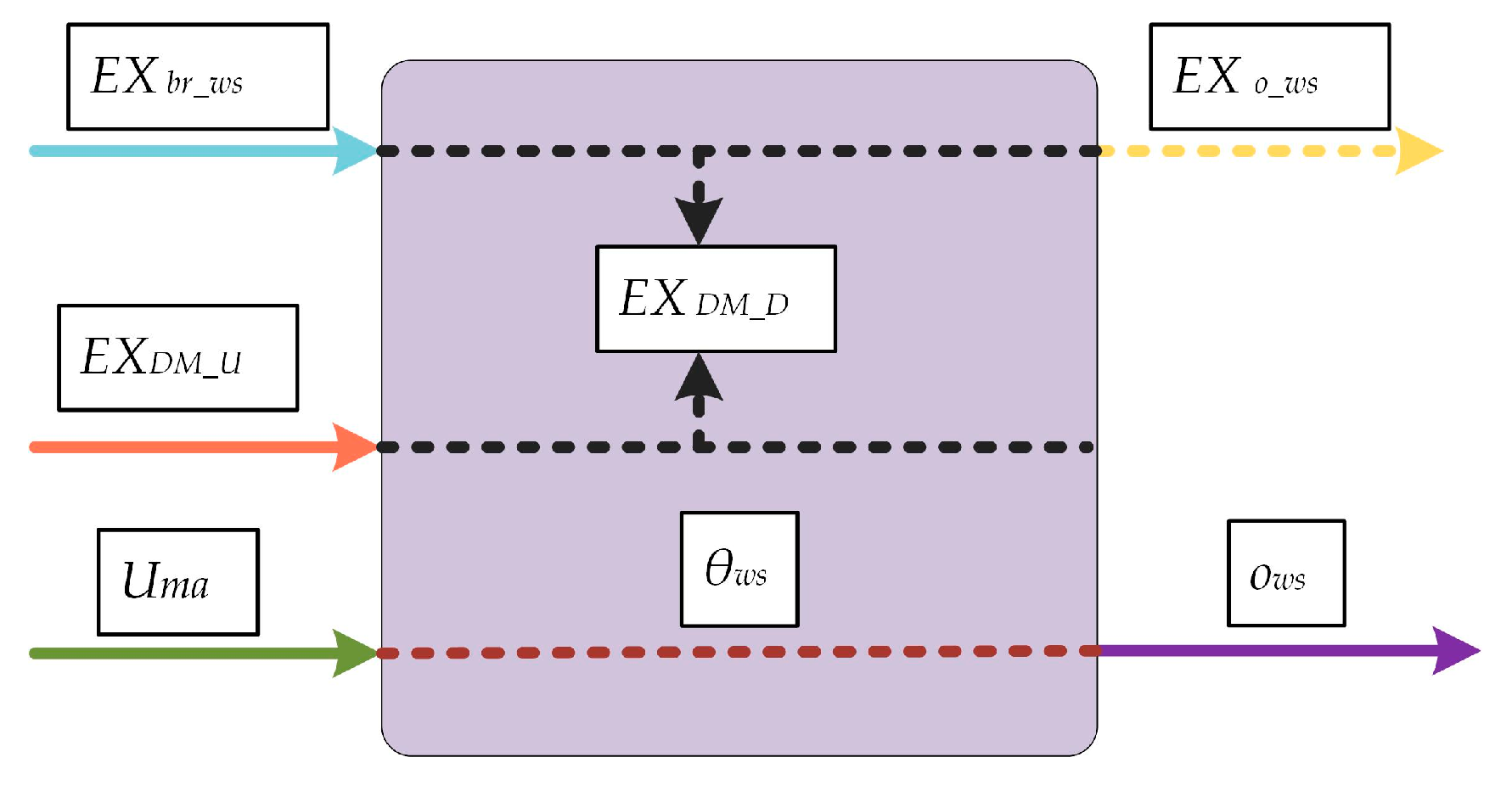
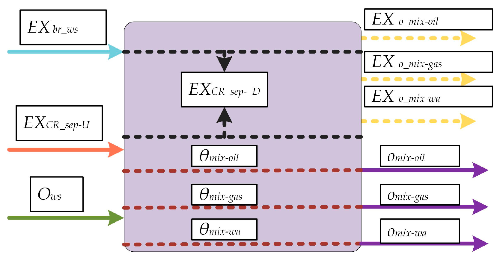
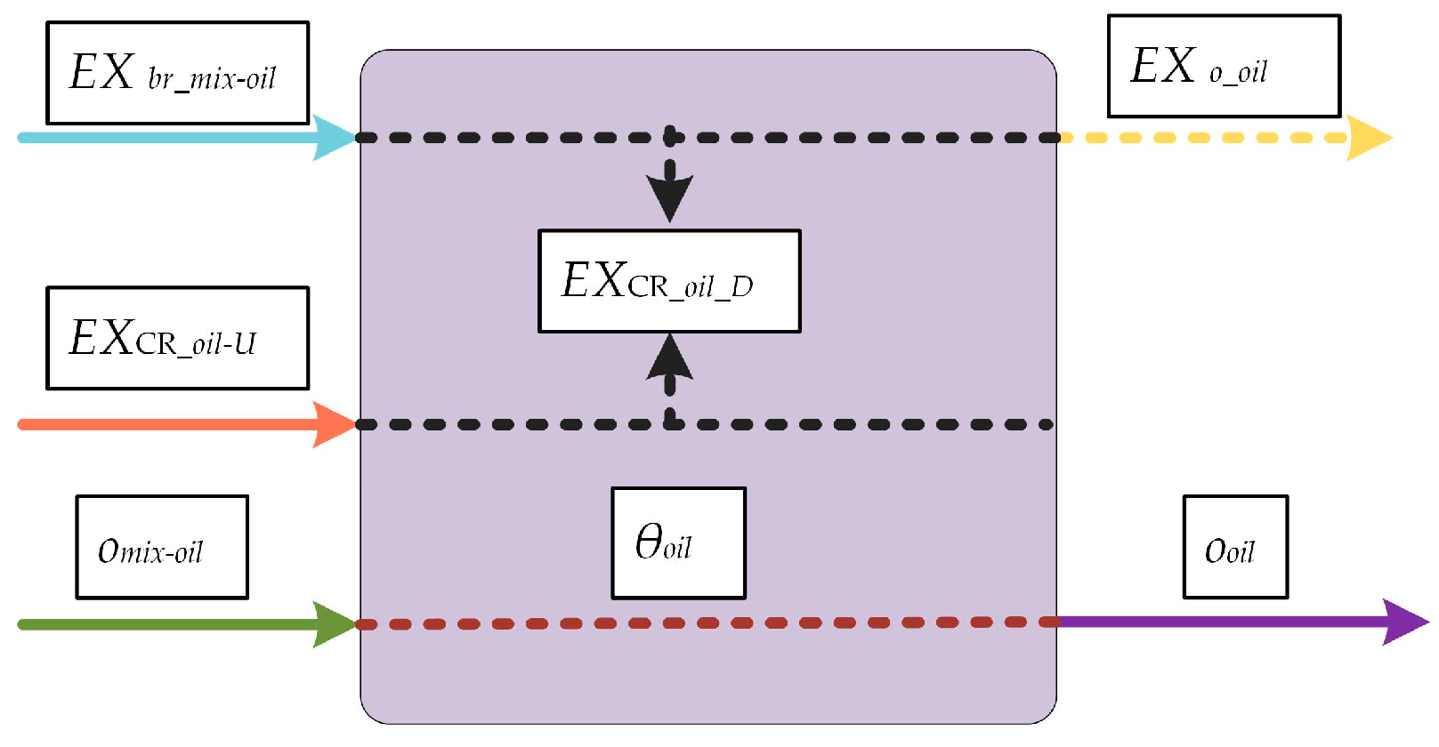
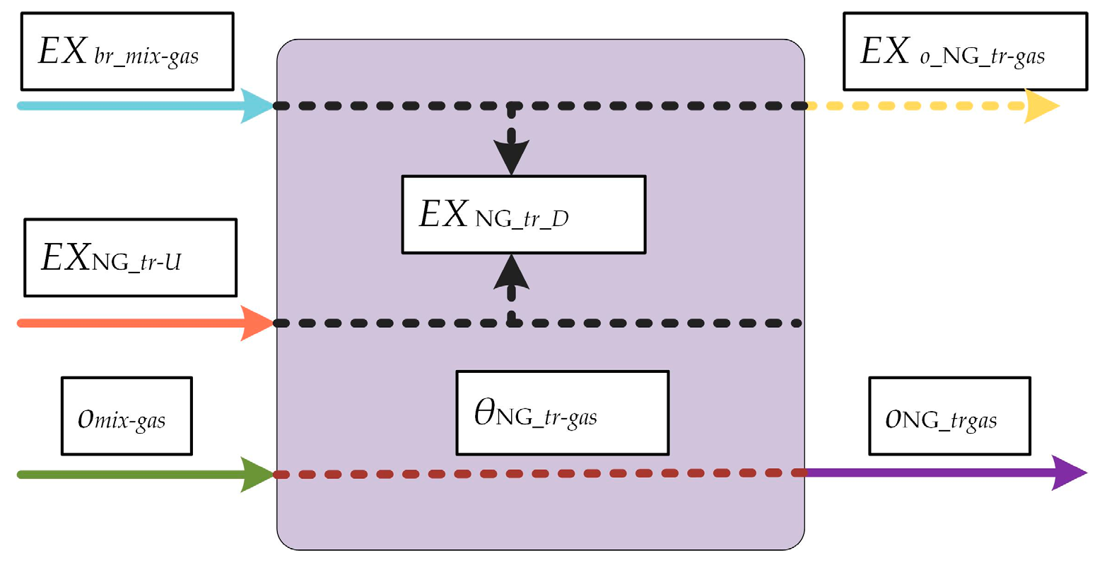
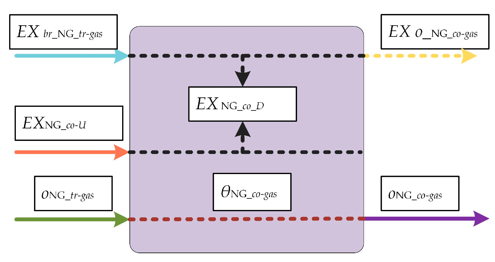
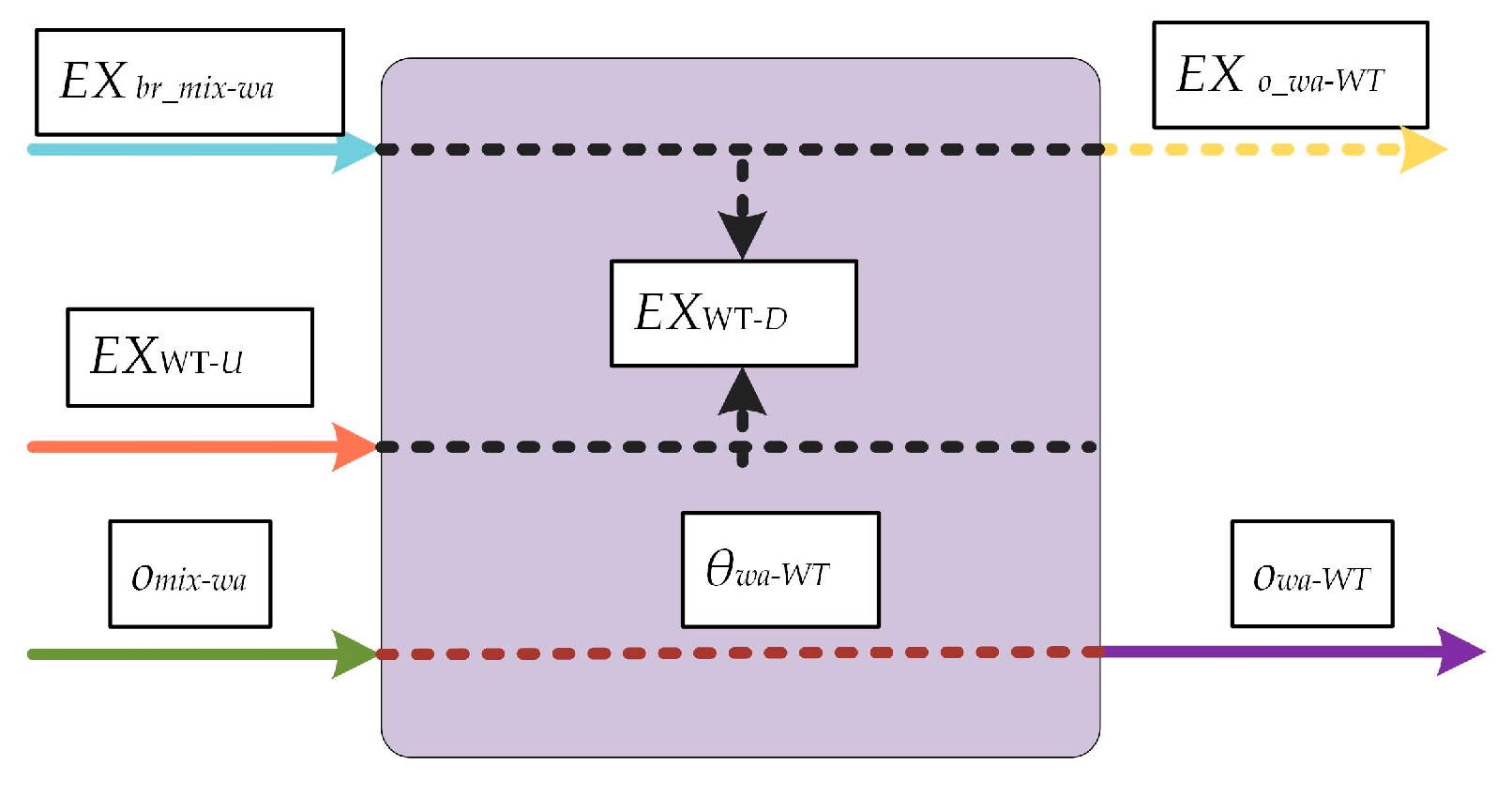
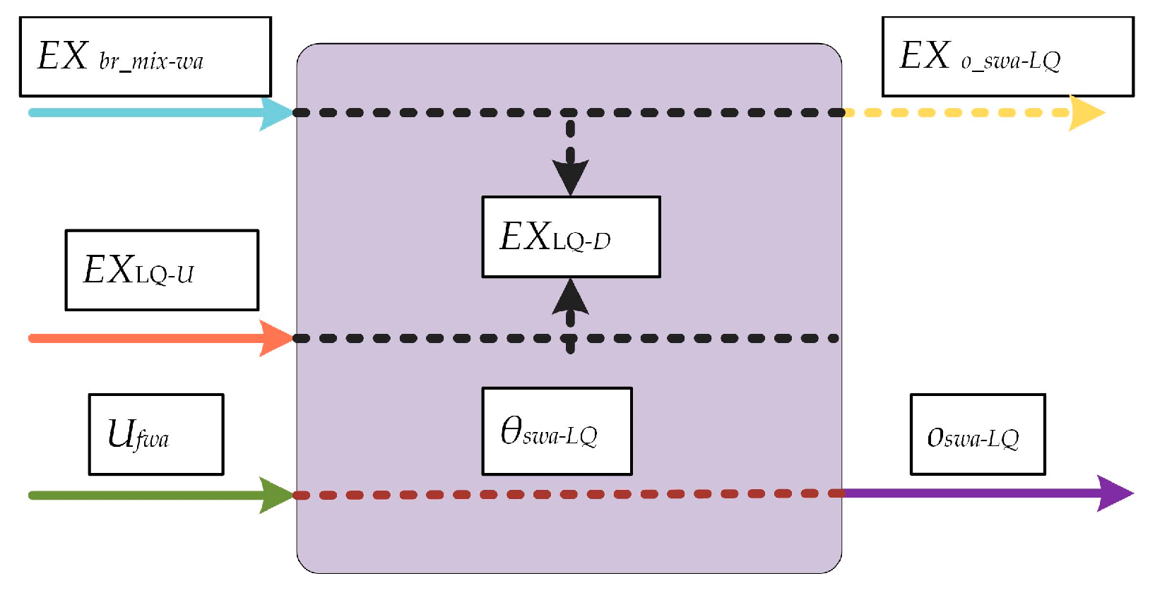
Figure 2. In the mapping of Process Section, an energy-material coupling element (EMCE) is defined, which represents the energy and non-energy relations of a sub-system. Figure 3 shows a basic framework of an EMCE. The detail expression of an EMCE is decided by its sub-system, which can be a factor or a function. A sub-system can be one EMCE or multiple EMCEs. Equation (2) shows the mathematic details of the Process Section in Figure 2. Here, an EMCE matrix, Z, is introduced to describe the relationship between production outputs and the consumption of energies and materials in the Process Section.
[ H F ] O = [ H 1 H r F r + 1 F n ] O = [ E θ E τ Z π Z ψ ] Z [ L U ] U ^ = [ e 11 e 1 r e 1 ( r + 1 ) e 1 m e r 1 e r r e r ( r + 1 ) e r m z ( r + 1 ) 1 z ( r + 1 ) r z ( r + 1 ) ( r + 1 ) z ( r + 1 ) m z n 1 z n r z n ( r + 1 ) z n m ] Z [ L 1 L r U r + 1 U m ] U ^
Under certain conditions, the outputs of the Process Section can be inputs for the Energy System, e.g., water reused, associated gas, or oil used as fuel directly. Hence, the Feedback Section represents such feedbacks from the Process Section to the inputs of the Energy System. The feedbacks are shown as Equation (3). Since not all of the outputs are fed back to the Energy System, B is a highly sparse matrix. When all entries of a column in B are zero, the corresponding production are not fed back to the input:
[ P U ] = [ I 1 I n I n + m ] I + [ b 11 b 1 n b 1 , n + m b n , 1 b n , n b n , n + m b n + m , 1 b n + m , n b n + m , n + m ] B [ O 1 O n O n + m ] O ,   ( 0 b 1 )
Therefore, Equations (1)–(3) represent the generalized energy and material flow model (GEMFM) of an IES and processing system illustrated as Figure 2.

4. Multi-objective Optimal Planning of the IESs

4.1. IESs Model

The proposed IES shown in Figure 1 consists of Co-firing gas turbines (GT), exhaust-fired-boilers (EFB), ORC, a two-level CO2 capture unit, a super-capacitor based energy storage, and pipeline system for gas and heat. According to the Section 3, an energy hub model is used to describe the IESs. The electricity output of Co-firing turbines is formulated as Equation (4):
E G T = G G T V A S η G T E + D G T V D O η G T E + H 2 V H 2 η G T E
The carbon dioxide emissions from the turbines is formulated as Equation (5):
C D E G T = λ G T ( G G T ) G G T + λ G T ( D G T ) D G T
The thermal energy contained in the exhaust of turbines is a function of electrical generation, shown as Equation (6):
Q G T = δ G T ( G G T ) G G T + δ G T ( D G T ) D G T + δ G T ( H 2 ) H 2
The thermal demands provided by the exhaust-fired-boiler through a thermal-oil system is:
Q o i l = ( G E F B V A S + D E F B V D O + α 1 Q G T ) η E F B Q
The carbon dioxide emissions (CDE) from the boiler is:
C D E E F B = λ E F B ( G E F B ) G E F B + λ E F B ( D E F B ) D E F B
The thermal energy in the exhaust from EFB to the ORC is (9):
Q O R C = α 2 ( δ E F B ( G E F B ) G E F B + δ E F B ( D E F B ) D E F B + Q E F B )
And the electricity generated by the ORC is (10):
E O R C = η O R C E Q O R C
The Pre-CO2 section converts a part of associated gas into the hydrogen as a fuel for GT and the CO2 to be absorbed, which consumes a proportion of power, i.e., EPre:
G Pr e E Pr e = σ Pr e ( G Pr e ) G Pr e H 2 + C D E Pr e
C D E Pr e = λ Pr e ( G Pr e ) G Pr e
H 2 = R h ( G Pr e ) G Pr e
The electrical and heat energy consumed in the CCS section is related the CO2 amount captured, i.e., CDECCS, as shown in Equations (14) and (15):
E C C S = k C C S E C D E C C S
Q C C S = k C C S Q C D E C C S
Here, Equations (16)–(18) denote the outputs of the hub:
L E = E G T + E O R C E S C E Pr e E C C S
L H = Q o i l
L C D E = C D E G T + C D E E F B + C D E Pr e C D E C C S
P 1 = G G T + G E F B + G Pr e
P 2 = D G T + D E F B
Hence, the model of the IESs is Equation (21) and its energy and emission flow mapping is shown as Figure 4, which corresponds to the ES section in Figure 2:
[ L E L H L C D E ] = [ r G T ( V A S η G T E + α 1 α 2 δ G T ( G G T ) η O R C E ) + r G B ( α 2 δ E F B ( G E F B ) η O R C E ) + r Pr e ( R h ( G Pr e ) V H 2 η G T E + α 1 α 2 δ G T ( H 2 ) R h ( G Pr e ) η O R C E σ Pr e ( G Pr e ) ) χ G T ( V D O η G T E + α 1 α 2 δ G T ( D G T ) η O R C E ) + χ G B ( α 2 δ E F B ( D E F B ) η O R C E ) r G T ( α 1 λ G T ( G G T ) η E F B Q ) + r E F B ( V A S η E F B Q ) + r Pr e ( α 1 δ G T ( H 2 ) R h ( G Pr e ) η E F B Q ) χ G T ( α 1 λ G T ( G G T ) η E F B Q ) + χ E F B ( V D O η E F B Q ) r G T ( λ G T ( G G T ) ) + r E F B ( λ E F B ( G E F B ) ) + r Pr e ( λ Pr e ( G Pr e ) ) χ G T ( λ G T ( D G T ) ) + χ E F B ( λ E F B ( D E F B ) ) ] [ P 1 P 2 ] [ 1 k C C S E 0 k C C S Q 0 1 ] [ E E C C D E C C S ]

4.2. Oil Extracting and Processing System Model (OEPS)

Figure 5 shows the OEPS of the actual offshore platform in this paper. This OEPS consists of drilling and mining system, crude oil process system, natural gas process system, water treatment system and living-quarters system, each of which includes one or more functional units. The OEPS shown in Figure 5 has two kinds of input: electricity and thermal energy provided by IESs; and materials for production and living, regularly supplied by a ship. OEPS output includes associated gas, oil product and water. The associated gas from OEPS is mostly delivered to IESs gas turbine for power generation or to waste heat boiler, and the redundant associated gas is burned off. Oil product from OEPS is delivered to the oil storage platform. The water recovered from OEPS can be re-injected, purified and discharged.
On the one hand, different functional units of OEPS have varied energy-material couplings and can be expressed using EMCE. Their energy-material input/output relationship can be described using EMCE matrix. On the other hand, the energy consumed by oil and gas production depends on the temperature, pressure, quality and velocity of the production process, in order to accurately calculate the energy consumption of each unit and specifically reflect the corresponding relationship between energy consumption and material production in each EMCE of the production process, this paper establishes an energy-material coupling model for each functional unit of OEPS using exergy analysis and derive EMCE matrix Z for OEPS from this model, so as to describe the relationship between OEPS production output and material & energy input.

4.2.1. Theory of exergy analysis for energy-material coupling model

Equation (22) expresses the exergy composition of a material flow x. Equations (23)–(26) are equations for calculating kinetic exergy, potential exergy, physical exergy and chemical exergy of material flow x [32]:
E X x = E X x k + E X x p + E X x p h + E X x c h
E X x k = 1 2 m x v x 2
E X x p = m x g H
E X x p h = ( h 1 h 0 ) T 0 ( s 1 s 0 )
E X x c h = R T 0 ln P 0 P 00
Equation (27) is an equilibrium expression of exergy for EMCE i. Equations (28) and (29) are equations for calculating product exergy, utilized exergy. This paper assumes there is no heat or mass loss due to exchange with environment, i.e., EXi−L = 0. Equation (30) is the equation for calculating exergy destruction for EMCE i, where εi is efficiency defect of EMCE i [33]:
E X i P = E X i U E X i L E X i D
E X i P = x E X o x x E X b r x
E X i U = ω i L E + ξ i L H
E X i D = ε i E X i U
Material flow direction and conversion relationship should be taken into consideration for offshore oil engineering design and planning. Equation (31) is a conversion relationship expression for input/output materials of EMCE i:
o x = θ x U y
Based on Equations (22)–(31), the general expression Equation (32) of EMCE matrix for EMCE i can be obtained:
O i = Z i U ^ i = [ E X i P o x ] = [ ω i ( 1 ε i ) ζ i ( 1 ε i ) 0 0 0 θ x ] [ L E L H U y ]

4.2.2. EMCE Matrix of Offshore Platform OEPS

Drilling and Mining System

Drilling and mining system includes the drilling and mining unit (DM) for oil extracting. This unit consumes certain raw material Uma and electricity exergy EXDM_U in producing per unit output of well stream ows. Its EMCE matrix is shown in Equation (33).
O D M = Z D M U ^ D M = [ E X D M P o w s ] = [ ω D M ( 1 ε D M ) 0 0 θ w s ] [ L E U m a ]

Crude Oil Process System

A crude oil process system comprises the three-phase separation unit (CR-sep) and the crude oil process unit (CR-oil). The CR-sep separates ows into mixed oil omix-oil, mixed associated gas omix-gas and mixed water omix-wa and delivers them respectively to crude oil processing unit, natural gas process system and water treatment system. Total amount of electricity and heat exergy consumed by this unit during separation is EXCR-sep_U. CR-oil processes mixed oil from CR-sep into oil product ooil for output; total amount of electricity and heat exergy consumed by this unit is EXCR_oil_U. EMCE matrices of CR-sep and CR-oil are shown in Equations (34) and (35):
O C R - s e p = [ E X C R - s e p - P o m i x - o i l o m i x - g a s o m i x - w a ] = Z C R - s e p U ^ C R - s e p = [ ω C R - s e p ( 1 ε C R - s e p ) ζ C R - s e p ( 1 ε C R - s e p ) 0 0 0 θ m i x - o i l 0 0 θ m i x - g a s 0 0 θ m i x - w a ] [ L E L H o w s ]
O C R - o i l = Z C R - o i l U ^ C R - o i l = [ E X C R - o i l - P o o i l ] = [ ω C R - o i l ( 1 ε C R - o i l ) ζ C R - o i l ( 1 ε C R - o i l ) 0 0 0 θ o i l ] [ L E L H o m i x - o i l ]

Natural Gas System

The natural gas system includes the natural gas treatment unit (NG-tr) and the natural gas compression unit (NG-co). The NG-tr dehydrates and deacidifies mixed associated gas omix-gas from the CR-sep to output combustible associated gas. The NG-co is responsible for natural gas compression transportation. Electricity and heat exergy consumed by this two unit, and their EMCE matrixes are shown in Equations (36) and (37):
O N G - t r = Z N G - t r U ^ N G - t r = [ E X N G - t r - P o N G - t r - g a s ] = [ ω N G - t r ( 1 ε N G - t r ) ζ N G - t r ( 1 ε N G - t r ) 0 0 0 θ N G - t r - g a s ] [ L E L H o m i x - g a s ]
O N G - c o = Z N G - c o U ^ N G - c o = [ E X N G - c o - P o N G - c o - g a s ] = [ ω N G - c o ( 1 ε N G - c o ) ζ N G - c o ( 1 ε N G - c o ) 0 0 0 θ N G - c o - g a s ] [ L E L H o N G - t r - g a s ]

Water Treatment System

Water treatment system includes a water treatment unit (WT). This unit processes mixed water omix-wa from CR-sep into wastewater owa_WT that complies with discharge standard, electricity exergy consumed by this unit is EXWT_U. Its EMCE matrix is shown in Equation (38):
O W T = Z W T U ^ W T = [ E X W T - P o w a - WT ] = [ ω W T ( 1 ε W T ) 0 0 θ w a - W T ] [ L E o m i x - w a ]

Living-Quarters System

The living-quarters system includes multiple living-quarters units (LQ). These units mainly consume fresh water Ufwa from external source and discharge properly wastewater oswa-LQ; electricity and heat exergy consumed by these units is EXLQ_U; the EMCE matrix is shown in Equation (39):
O L Q = Z L Q U ^ L Q = [ E X L Q - P o s w a - L Q ] = [ ω L Q ( 1 ε L Q ) ζ L Q ( 1 - ε L Q ) 0 0 0 θ s w a - L Q ] [ L E L H U f w a ]

EMCE Matrix of OEPS

Therefore, offshore platform PS can consist of the above 6 EMCE functional units and the production tasks of the offshore platform can be fulfilled through coordination between these functional units. Based on Equations (33)–(39), EMCE matrix expression Equation (40) for the offshore platform OEPS can be derived:
O O E P S = [ E X C R - o i l - P E X N G - c o - P E X W T - P E X L Q - P o o i l o N G - co - g a s o s w a - W T o s w a - L Q ] = Z O E P S U ^ O E P S = [ ω C R - o i l ( 1 ε C R - o i l ) ζ C R - o i l ( 1 ε C R - o i l ) 0 0 ω N G - c o ( 1 ε N G - c o ) ζ N G - c o ( 1 ε N G - c o ) 0 0 ω W T ( 1 ε W T ) 0 0 0 ω L Q ( 1 ε L Q ) ζ L Q ( 1 ε L Q ) 0 0 0 0 θ o i l θ m i x - o i l θ w s 0 0 0 θ N G - co - g a s θ N G - tr - g a s θ m i x - g a s θ w s 0 0 0 θ s w a - W T θ m i x - w a θ w s 0 0 0 0 θ s w a - L Q ] [ L E L H U m a U f w a ]
EMCE material flow exergy calculation and input/output material flow conversion relationship on offshore platform OEPS can be seen in Appendix A and Appendix B.

4.3. Multi-Objective Stochastic Optimization Model

4.3.1. Uncertainty Analysis

The energy system serves the production system in offshore platform. Therefore, before the energy system planning, it is necessary to pre-determine an oil and gas production plan based on factors such as the amount of oil and gas exploration, the quality of crude oil quality, and then the electricity and thermal consumption of production system can be calculated according to the production process. Since the planning period of offshore oil and gas project is very long, generally 20–25 years, improvements in mining techniques or inaccurate reservoir estimates result in significant deviations between actual production and estimated values, which leads to uncertainties. The operational data of the Bohai platform indicates that such deviations will lead to frequent start-up of standby units, which will reduce the stability of the offshore platform micro-grid and cause great economic losses. Therefore, it is necessary to consider this uncertainty when planning.
This paper considers the impact of uncertainty in oil extraction on optimization of the energy systems, using the IESs and OPES model established in Section 4.1 and Section 4.2. According to Figure 4, Figure 5 and Equations (21) and (40), IESs output electricity and heat are energy input for OEPS, while some associated gas from OEPS is fuel input for IESs. Therefore, IESs input and load are correlated. The deviations between the actual value of the electric load, the heat load, and the associated gas output and the estimated value are treated as random variables in this paper. And the three random variables were assumed to follow a normal distribution [34], multi-dimensional Gaussian Copula function [35] is selected to describe the relevance of variables, as shown in Equation (41):
{ c ( u 1 , , u n ) = 1 | A cov | 1 / 2 exp q T ( A cov 1 I ) q 2 q = ( q 1 , , q n ) T , q i = Φ 1 ( u i )

4.3.2. Objective Function

Considering cost-effectiveness and environmental performance are main indicators in offshore oil engineering, the proposed IESs optimization is aimed at minimizing total cost and total carbon dioxide emissions during planning period. The objective function is shown in Equation (42). Equation (43) is an equation for calculating fTTC and fTCDE:
min ( F ) = min ( f T T C , f T C D E ) T
{ f T T C = y = 1 Y f T A C y f T C D E = y = 1 Y f C D E y f T A C y = f C C y + f M C y + f O C y

4.3.3. Constraints

Constraints of the proposed IESs optimization planning include energy-material equilibrium of IESs and OEPS as shown in Equations (21) and (40), gas-network pipeline equilibrium, electricity-network equilibrium and thermal-network equilibrium as shown in [34]. The inequation is shown in Equation (44), and the chance constraints of gas flow, injection power and thermal medium flow on nodes of each network are shown in Equations (45)–(47):
I e q min I e q I e q max
P r { ω i min ω i ω i max } β 1
P r { P s , i min P s , i P s , i max } β 2
P r { M s , i min M s , i M s , i max } β 3

4.3.4. Optimization Method and Solving Steps

To sum up, the proposed multi-objective stochastic optimization model is expressed as Equation (48):
{ o b j .     min ( F ) = min ( f T T C , f T C D E ) T s t .      ( 21 ) , ( 40 ) , ( 44 ) , ( 45 ) , ( 46 ) , ( 47 )
With a long planning period for offshore oil engineering, optimized objectives in this paper are calculated in two steps in order to ensure accuracy when solving the objective function. In step one, fTAC and fCDE of the offshore platform during the maximum load are optimized, optimal capacity solution set of IESs component is obtained in feasible region. The target values are normalized separately and summed according to the 50% weighting factor, the solution with the smallest value is selected as the best one.
The decision variables of the optimization model are mainly composed of the energy consumption and output power of each unit, as well as the load, which are all continuous variables, as shown in Table 1. Energy consumption and output power of each unit are deterministic variables, and electric load, thermal load and associated gas input are uncertain variables.
At present, gas turbines are widely used in offshore platforms, and there are many products to choose from the market. However, technologies such as CCS\ORC\WHRU have not been widely used in offshore engineering and there are quite few units to choose from, which can be customized according to the conditions. When selecting equipment, the load rate is often selected as reference indicator. The higher the load rate, the better the economy, but the load rate is not allowed to exceed 0.95. Equation (49) is equation for calculating the load rate:
r = o p d p × 100 %
Hence, in step two, the model and combination of the equipment are determined according to the load rate.
Finally, average annual cost and annual emissions for each year in the planning period are calculated based on the design parameters selected, leading to fTTC and fTCDE in the planning period for the offshore platform. The multi-objective genetic algorithm NSGAII and Monte Carlo simulation are used in this paper to solve the problem, and statistical sampling and probability distribution functions are used to simulate the effects of uncertain variables [35]. The flow chart of multi-objective stochastic optimization is shown in Figure 6.

5. Results

This study is based on an offshore oil extraction and processing site platform in the Bohai Sea area. 
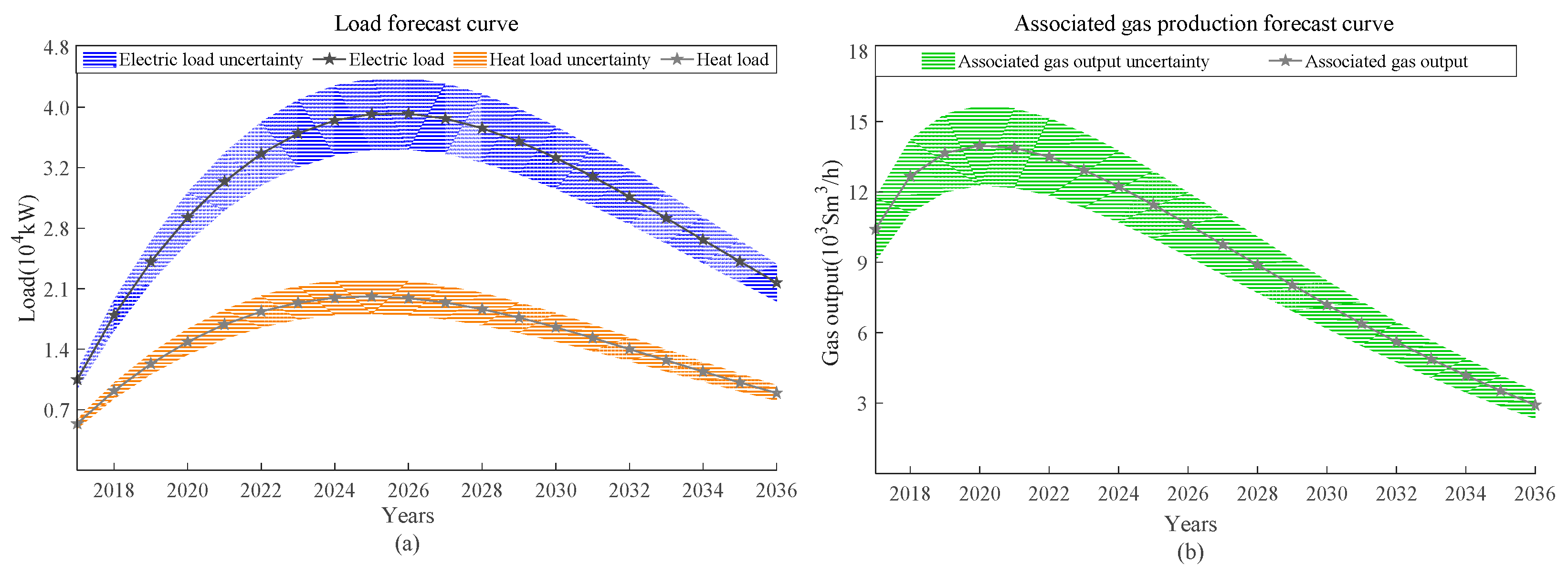
Figure 7 shows the estimated curve of electric and thermal load demands and associated gas production for this platform in the coming 20 years. According to Figure 7a, electric load is over twice the thermal load, indicating the gas turbine on this platform produces abundant residual heat from flue gas. According to Figure 7a, load demand in the planning period varies significantly, with a different reference load each year and culminating in the middle of the production period. To ensure the planned equipment capacity can meet the load demand of the platform in any period, this paper conducts verification against maximum reference load estimated for the offshore platform, i.e., electric load of 44,157 kW, thermal load of 14,100 kW and associated gas production of 9000 Sm3/h. According to forecast in Figure 7b, associated gas production is high in early production period but falls sharply afterward, suggesting associated gas may fall short of the demand of gas turbine in the middle and later periods of production, thus requiring diesel supply. Meanwhile, actual oil extraction may be different from the plan, which must be considered in planning. This study assumes that the mean of the random variables is ±10% of the predicted value, as shown in Figure 7a,b.
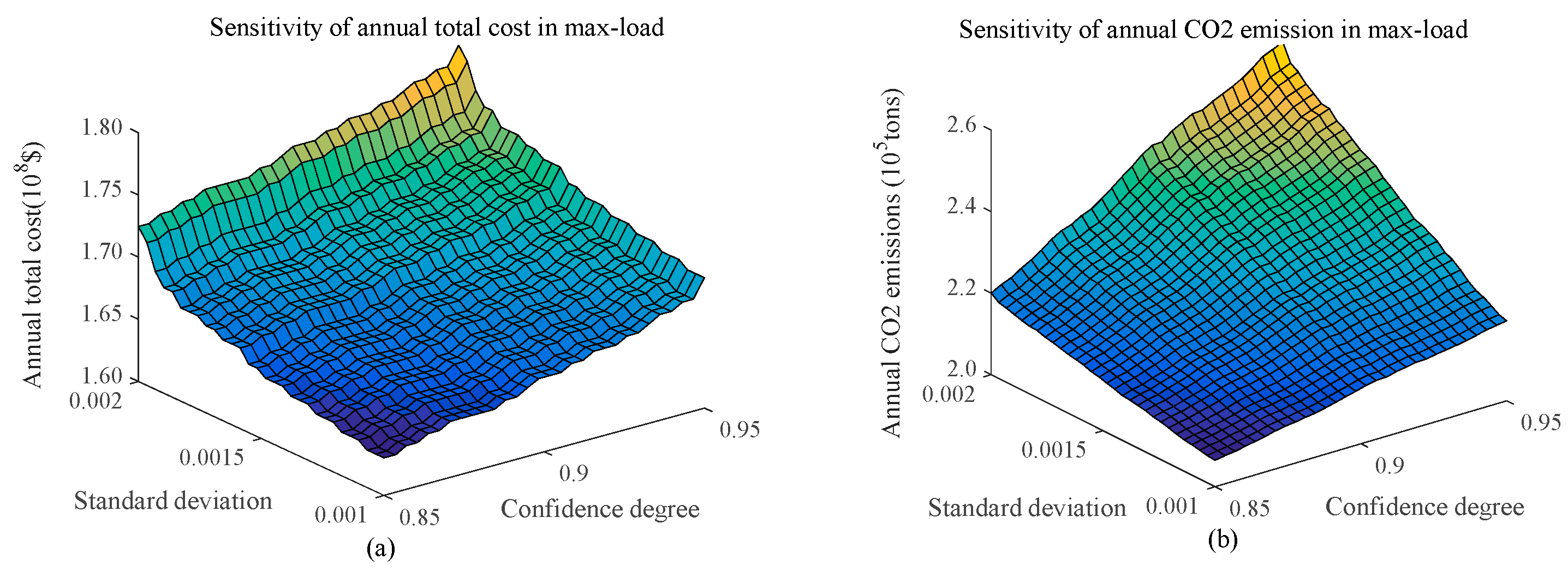
Figure 8 shows IESs sensitivity analysis at maximum reference load. Figure 8a,b show analysis of sensitivity of annual total cost and annual carbon dioxide emissions. The standard deviation of random variables are 0.001–0.002 times the mean values, and confidence level of chance constraint discussed in this paper are 0.85–0.95. Figure 8a,b show an increase in either joint distribution variance or confidence level of chance constraint leads to a rise in annual total cost and annual carbon dioxide emissions. Therefore, to address the uncertainty in offshore production and load, more investment needs to be made into the system to ensure stable production; meanwhile, ignoring the uncertainty in process and load may make IESs unable to satisfy the requirement of stable production. Since offshore platform IESs require high levels of safety and stability, this paper conducts optimization under a chance constraint confidence level of 0.95 and variance of 0.002.
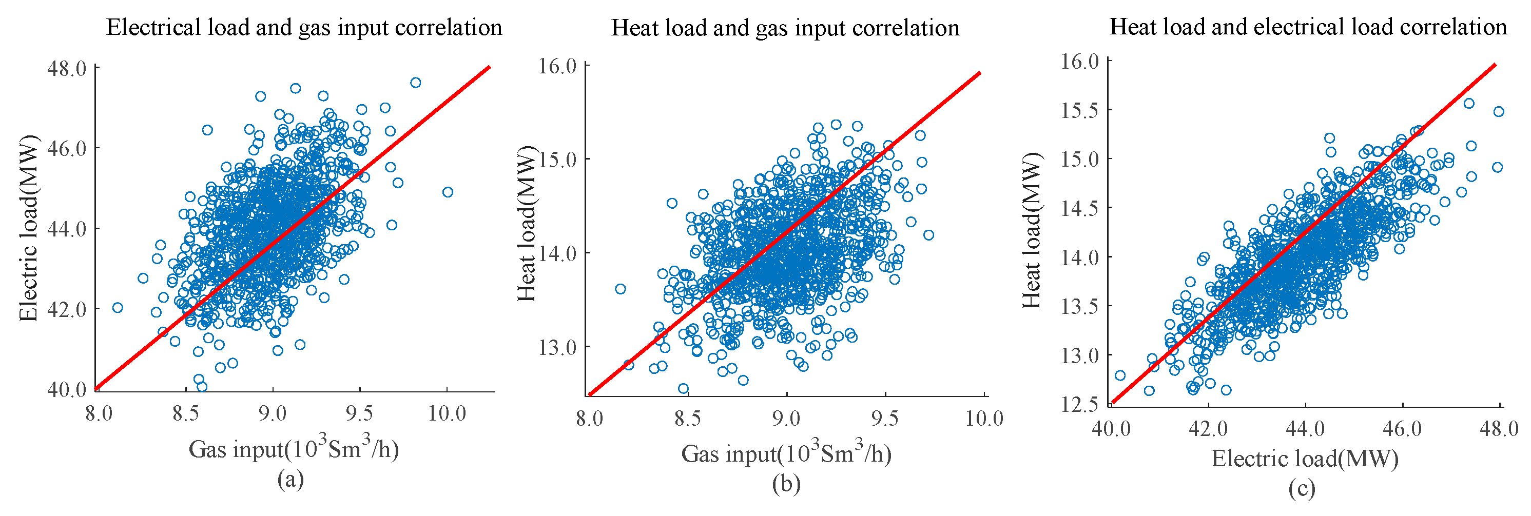
In a complicated and ever changing process of actual oil extraction, the changing gas-oil ratio and oil-water ratio make accurate forecast of associated gas production impossible, with an impact on IESs operating cost and CO2 emissions. In addition, the electricity and thermal consumption of the offshore platform depends mainly on the real-time operating conditions of OEPS. Figure 9 shows data samples of correlations between associated gas production and electric load (Figure 9a), between associated gas production and thermal load (Figure 9b), between electric load and thermal load (Figure 9c). Distributed data closer to center line suggests a higher correlation between variables. It can be seen from the Figure 9 that the electric and thermal loads are highly correlated to each other, while they have roughly the same correlation with the associated gas.
This paper adopts three methods to planning and design of energy supply system for this platform. Method 1 is an existing method for offshore platform; its energy supply system is Combined Heat and Power (CHP) system consisting of dual-fuel gas turbine and waste heat boiler; its equipment capacity is calculated using the method specified in design code [6]. This method is deterministic planning. Moreover, Method 1 takes account of only cost-effectiveness while CO2 emissions are not considered. Method 2 offers a stochastic planning method that takes account of random effects of electric and thermal loads and associated gas production, on the basis of Energy-Hub model as shown in Figure 4. Method 3 offers a stochastic planning method that takes account of correlation between IESs and OEPS, on the basis of Generalized Energy and Material Flow Model (GEMFM) as shown in Figure 2.
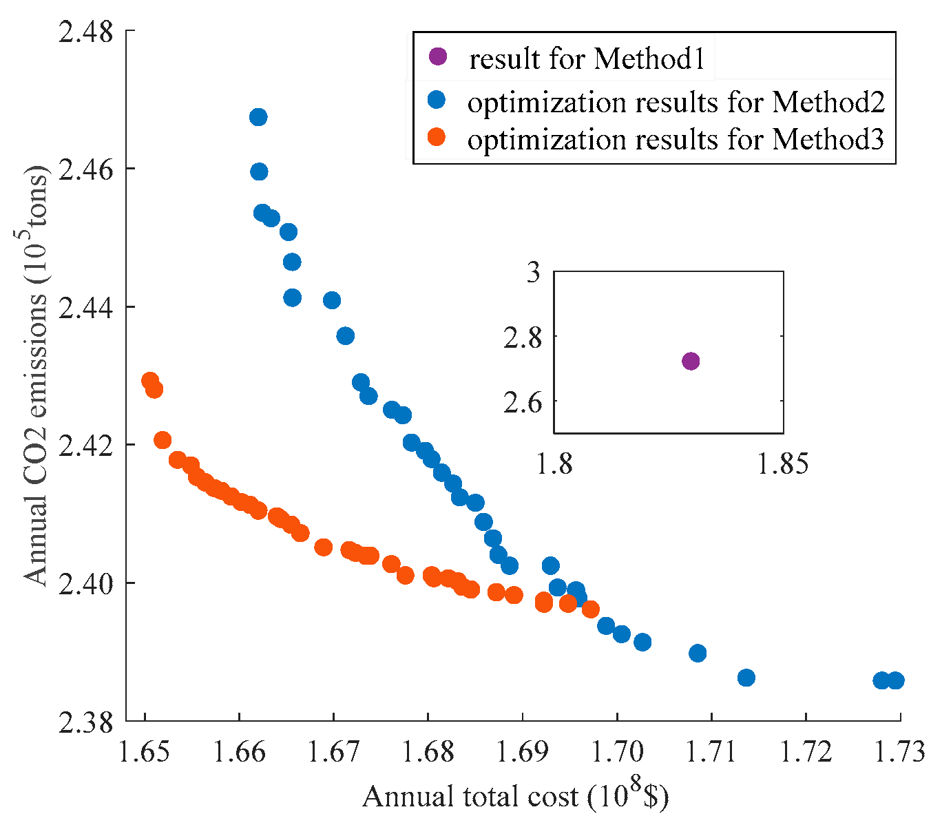
Figure 10 shows the planning results of annual average cost and annual emissions using the three methods at maximum reference load. According to Figure 10, the results of methods 2 and 3 are better than those of Method 1, because: Method 1 is deterministic, requiring large spare capacity to ensure stability in energy supply for OEPS; in comparison with IESs, CHP is free of low-temperature waste heat recovery device (ORC) and emission reduction measures (CCS), resulting in more energy consumption and CO2 emissions in Method 1 than in methods 2 and 3. Figure 10 also suggests better results from Method 3 than from Method 2. This is because: when fluctuation in associated gas production affects electric and thermal loads of IESs, IESs can quickly respond to load fluctuation through SC charging/discharging to meet the electricity demand of OEPS; the cascaded utilization of waste heat and diesel coordination and compensation in IESs weakens the secondary impact of fluctuation in associated gas production on load. Therefore, it is helpful to consider the impact of IESs -OEPS correlation on IESs optimization.
Table 2 shows the power and heat dispatch in energy system using three methods under maximum reference load. According to Table 2, in Method 1, the dual-fuel gas turbine and waste heat boiler undertake all energy supply on the offshore platform; in methods 2 and 3, mixed gas turbine supplies about 90% of electricity for the platform as core equipment of power supply, while ORC supplies about 12% of electricity using low temperature waste heat power generation. High temperature waste heat from the gas turbine is far greater than all the heat IESs needs, so the waste heat boiler can meet thermal load for the platform without refueling. Low temperature waste heat available to ORC is in a large amount, but low temperature heat sources are not fully used due to restrictions on ORC efficiency. Pre-CO2 and CCS processes consume about 5.8% of electricity; CCS process consumes about 6.8% of heat energy.
Table 3 shows the comparison of energy system performances using three methods under maximum reference load. According to Table 3, total power generating capacity and heat generating capacity in methods 2 and 3 are larger than in Method 1, consuming less total calorific value of fuel than in Method 1. This is because IESs generates power using low and medium temperature tail gas from the boiler through ORC, resulting in higher energy efficiency and lower fuel consumption. In this case, associated gas production is not enough to meet the fuel demand of gas turbine, so diesel needs to be supplied. To ensure stable energy supply, the use ratio of associated gas is set as 0.9 or smaller (taken as 0.9 in this paper) while the unused portion is burned off.
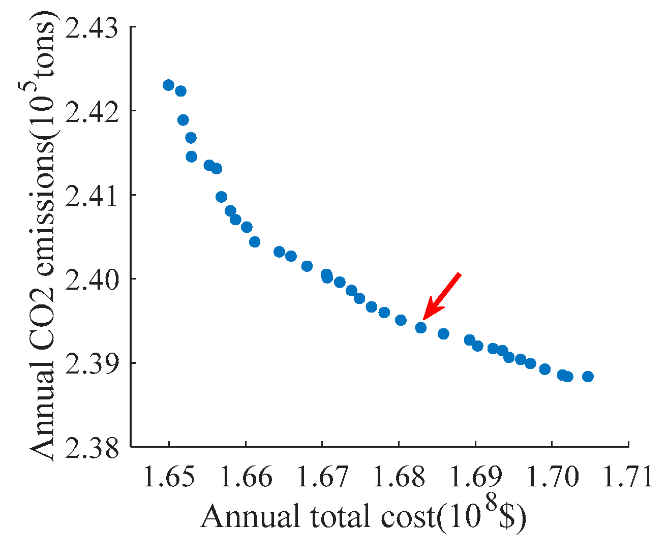
Figure 11 shows distribution of optimal solution set using Method 3. According to this figure, annual carbon dioxide emissions and annual total cost are in conflict with each other, forming a non-dominated relationship. The best solution is pointed by the red arrow. Table 4 gives equipment components of energy system and the capital cost of the equipment components in the three methods. This article selects a co-firing gas turbine made by Siemens, which specific parameters are shown in Appendix C.
Table 5 presents proportions of electricity and heat consumed by five subsystems of the offshore platform OEPS under maximum reference load in 2026. The drilling and mining system consumes the most electricity exergy, because the electric submersible pump for extraction of mixed fluid consumes large amounts of electricity. Crude oil process system consumes the most heat exergy because its three-phase separation unit and crude oil processing unit need large amounts of heat to meet the requirements for mixed fluid separation and crude oil processing.
Table 6 shows the exergy consumption of OEPS five subsystems using three methods under maximum reference load. According to Table 6, OEPS consumes more heat and electricity exergy in methods 2 than in Method 3. The underline reason is that the associated gas production is less and OEPS process less oil and gas when the correlation is considered, hence it consumes less exergy energy. 
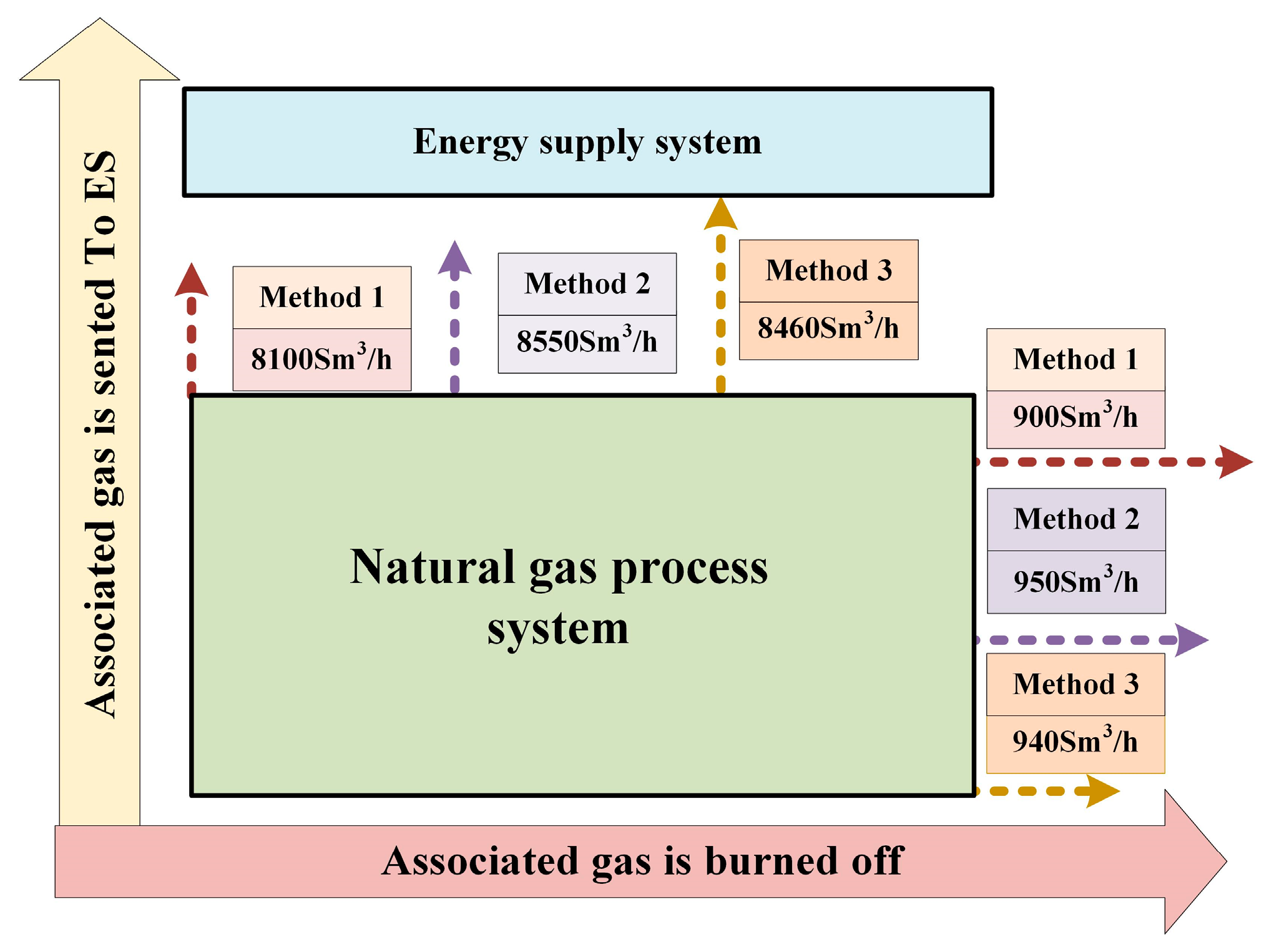
Figure 12 shows the dispatch of associated gas in the three methods. According to Figure 12, the dispatch of associated gas can be divided into two parts: one part is delivered to IESs for power generation whereas the other is burned off. In general, comparison with Method 390 Sm3/h more associated gas are allocated to IESs by Method 2, which means 332.5 kW of exergy, but it consumes more 1844 kW.
Table 7 gives the comparison of total cost and total CO2 emissions in a 20-year planning period using the three methods. Method 3 entails the minimum total capital cost, total maintenance cost, total operating cost and total CO2 emissions over the planning period, because it significantly cuts acquisition and installation costs for gas turbine and requires minimum diesel consumption over the planning period. Compared with Method 1, Method 2 can reduce 11.21% and 12.4% the total cost and CO2 emissions, respectively. And the reduction of total cost and CO2 emissions are 18.9% and 17.3% by Method 3, respectively. Hence, Method 3 is the most economy and environmental friendly planning method.

6. Conclusions

Studies on optimization and uncertainty of the integrated energy system have become a hot topic. This paper investigates the long-term plan and uncertainty of IESs for offshore platforms. It is found that the uncertainty produced in the OEPS of the offshore platform leads to fluctuations of input energy and load in the IESs of the offshore platform, and it is the key factor for the IESs uncertainty. OEPS and IESs are closely related in terms of structure, specifically, OEPS is the “electric and thermal loads’ for IESs, while IESs is the “associated gas load” for OEPS. As a result, the input energy and load uncertainty of IESs are relevant, which is the characteristic of the offshore platform. Regarding this characteristic, a generalized energy and material flow model comprising energy-hub, process-hub and feedback-hub is proposed in this paper. An input/output conversion matrix is established according to energy conservation, exergy equilibrium and material conservation theories. It can address the special structure of coupled output and input ends of energy-material flow. Besides, the proposed model can analysis the uncertainty and correlation in each process. What’s more, a multi-objective stochastic planning method is developed to achieve the system’s optimization.
IESs obtained according to the proposed method highlights thermal-electric coupling and cascaded utilization of waste heat. The high-temperature waste heat from gas turbine is used to meet heat load requirements and the low-temperature waste heat is used for power generation to bridge the gap due to the decreased capacity of gas turbine and adoption of CCS. Introduction of ORC could reduce the installed capacity of gas turbine, thus cutting IESs construction and maintenance costs. Planning results in this paper represent 17.3% less CO2 emissions due to less use of primary energy and deployment of CCS.

Author Contributions

Conceptualization, A.Z. and H.Z.; Methodology, A.Z.; software, H.Z.; validation, M.Q., W.Y, and X.J.; writing—original draft preparation, M.Q., A.Z., H.Z. and W.Y.; writing—review and editing, J.W. and M.Q.; supervision, J.W.

Funding

This research was supported by the Chinese National Key Research and Development Plan under Grant 2017YFE0112600 and the China Postdoctoral Science Foundation under Grant 2014M562335.

Conflicts of Interest

The authors declare no conflict of interest.

Nomenclature

Sets and Indices
Lthe set of energy outputs
Pthe set of energy inputs
Cthe coupling matrix of the Energy Section
Sthe set of energy storages
Pmthe mth input energy carrier of the Energy Section
Lnthe nth output energy carrier of the Energy Section
cnmthe coupling factor which defines the coupling between Pm and Ln
Othe set of the production outputs
Uthe set of non-energy inputs
Zthe coupling matrix of the Process Section.
Eθthe sub-matrix which reflect the relationship between energy and energy
Eτthe sub-matrix which reflect the relationship between energy and non-energy
Zπthe sub-matrix which reflect the relationship between non-energy and energy
Zψthe sub-matrix which reflect the relationship between non-energy and non-energy
Umthe mth non-energy inputs to the Process Section
Hrthe rth output energy carrier of the Process Section
Fnthe nth output non-energy carrier of the Process Section
ern/znnthe coupling factor which defines the coupling of an energy-material coupling element (EMCE)
ukjthe kth non-energy input of the jth EMCE
lwjthe wth energy input of the jth EMCE
fjjthe jth non-energy output of the jth EMCE
hjjthe jth energy output of the jth EMCE
Ithe sets of energies imported to the Energy Section
Bthe feedback matrix
bnmthe feedback factor between Om and Ln
Parameters and Variables
Exelectricity generation or consumption of unit x
Gxassociated gas input to unit x
VAScalorific value of associated gas, 38 MJ/Sm3
VDOcalorific value of diesel oil, 42 MJ/kg
ηExelectricity conversion efficiency of unit x
ηQxelectricity conversion efficiency of unit x,
Dxdiesel oil input to unit x
H2hydrogen inputs
CDExCO2 emission of unit x
λx(.)emission function of the input material x
Qxheat generated/consumed by unit x
δx(.)heat function of the input material x
αxwaste heat utilization ratio by x
σpre(Gpre)power consuming function of Pre-CO2
Rh(Gpre)hydrogen generation function of Pre-CO2
kECCSelectrical consumption of CCS, 0.256 kW/kg
kQCCSheat consumption of CCS, 0.38 kW/kg
LEthe electricity output of the energy section
LHthe heat output of the energy section
LCDEthe CO2 output of the energy section
P1the total amount of associated gas input
P2the total diesel input
EXx_kkinetic exergy of material flow x
EXx_ppotential exergy of material flow x
EXx_phphysical exergy of material flow x
EXx_chchemical exergy of material flow x
EX x_Pproduct exergy for EMCE i
EXi_Uutilized exergy for EMCE i
EX i_Lexergy loss for EMCE i
EX i_Dexergy destruction for EMCE i
EX o_xoutput exergy of material flow x
EX br_xinput exergy of material flow x
mxmass flow rate of fluid x
vxflow speed of fluid x
ggravitational acceleration
Hrelative height of fluid x
hspecific enthalpy
sspecific entropy
T0the ambient temperature
Rmolar gas constant on material flow x
P0function of environmental pressure
P00partial pressures of material flow x
ωicoefficients of electricity consumed by EMCE i
ξicoefficients of heat consumed by EMCE i
oxoutput material flow x of EMCE i
θxthe coefficient of converting
Uyinput material flow y of EMCE i
Oioutput matrix of EMCE i
ZiEMCE matrix of EMCE i
Uiinput matrix of EMCE i
QXo-xmass flow rate of fluid x
GXo-xvolume flow rate of fluid x
VXo-xoutput speed of fluid x
Pa0ambient pressure
Pax-1inlet pressure of fluid x
Pax-2outlet pressure of fluid x
Tx-1inlet temperatures of fluid x
Tx-2outlet temperatures of fluid x
Hexowsaverage liquid depth
Cpx-1 constant-pressure specific heat of fluid x at inlet
Cpx-2 constant-pressure specific heat of fluid x at outlet
c(.)probability density function of Copula
uithe specific value of the ith uniformly distributed random variable
Acovcovariance matrix
Iunit matrix
qinormal integral
qvector quantity comprising qi
Φ−1inverse cumulative distribution function
fTTCtotal cost
fTCDEtotal carbon dioxide emissions
Yproject planning period
fTACyannual total cost in the yth year
fCDEyannual carbon dioxide emissions in the yth year
fCCycapital cost in the yth year
fMCymaintenance cost in the yth year
fOCyoperating cost in the yth year
Ieqequation constraint set
Ieqmaxupper limits of inequation constraint set
Ieqminlower limits of inequation constraint set
Pr{.} probability of satisfied inequation in {.}
ωigas flow at node i
ωimax upper limits of gas flow at node i
ωiminlower limits of gas flow at node i
Ps,iinjection power at node i
Ps,imaxupper limits of injection power at node i
Ps,iminlower limits of injection power at node i
Ms,isupply mass flow rate at node i
Ms,imaxupper limits of supply mass flow rate at node i
Ms,iminlower limits of supply mass flow rate at node i
βconfidence level of chance constraint
rthe rate load
opoperating power
dpdesign power
Abbreviations
GTCo-firing gas turbines
EFBexhaust-fired-boilers
ORCorganic Rankine cycle
CCSCO2 capture and storage system
SCsuper-capacitor
ASAssociated gas
DODiesel oil
PrePre-CO2 capture unit
CDEcarbon dioxide emissions
DMthe drilling and mining unit
wswell stream
CR-septhe three-phase separation unit
CR-oilthe crude oil process unit
NG-trthe natural gas treatment unit
NG-cothe natural gas compression unit
WTthe water treatment unit
LQthe living-quarters unit

Appendix A

Appendix A.1. Exergy Formula for DM

E X o - w s = Q X o - w s ( P a w s 2 P a 0 ) T 0 T w s 2 + G X o - w s g H e x o - w s + 1 2 G X o - w s V X o - w s 2
E X b r - w s = Q X b r - w s ( P a w s 1 P a 0 ) T 0 T w s 1
E X D M P = E X o - w s E X b r - w s
E X D M - U = ω D M L E
E X D M - D = δ D M E X D M - U .
Figure A1. Process flowsheets of DM.
Energies 12 00756 g0a1

Appendix A.2. Exergy Formula for Crude Oil Process System

Appendix A.2.1. Exergy Formula for CR-sep

E X C R - s e p - P = E X o - m i x - o i l + E X o - m i x - g a s + E X o - m i x - g a s E X o - w s
E X o - m i x - o i l = Q X o - m i x - o i l ( P a m i x - o i l 2 P a 0 ) T 0 T m i x - o i l 2 + G X o - m i x - o i l g H e x o - m i x - o i l + 1 2 G X o m i x - o i l V X o - m i x - o i l 2
E X o - m i x - w a = Q X o - m i x - w a ( P a m i x - w a 2 P a 0 ) T 0 T m i x - w a 2 + G X o - m i x - w a g H e x o - m i x - w a + 1 2 G X o - m i x - w a V X o - m i x - w a 2
E X o - m i x - g a s = Q X o - m i x - g a s ( P a m i x - g a s 2 P a 0 ) T 0 T m i x - g a s 2 + G X o - m i x - g a s C p m i x - g a s 2 [ ( T m i x - g a s 2 T 0 ) - T 0 ln T m i x - g a s 2 T 0 ]
E X C R - s e p - U = ω C R - s e p L E + ξ C R - s e p L H
E X C R - s e p - D = ε C R - s e p E X C R - s e p - U .
Figure A2. Process flowsheets of CR-sep.
Energies 12 00756 g0a2

Appendix A.2.2. Exergy Formula for CR-oil

E X C R - o i l - P = E X o - o i l E X b r - o i l
E X b r - o i l = E X o - m i x - o i l
E X o - o i l = Q X o - o i l ( P a o i l 2 P a 0 ) T 0 T o i l 2 + G X o - o i l g H e x o - o i l + 1 2 G X o - o i l V X o - o i l 2
E X C R - o i l - U = ω C R - o i l L E + ξ C R - o i l L H
E X C R - o i l - D = ε C R - o i l E X C R - o i l - U .
Figure A3. Process flowsheets of CR-oil.
Energies 12 00756 g0a3

Appendix A.3. Exergy Formula for Natural Gas System

Appendix A.3.1. Exergy Formula for NG-tr

E X N G - t r - P = E X o - N G - t r - g a s E X b r - m i x - g a s
E X b r - m i x - g a s = GX b r - m i x - g a s C p m i x - g a s 1 [ ( T m i x - g a s 1 T 0 ) T 0 ln T m i x - g a s 1 T 0 ] + Q X b r - m i x - g a s ( P a m i x - g a s 1 P a 0 ) T 0 T m i x - g a s 1
E X o - N G - t r - g a s = GX o - N G - t r - g a s C p N G - t r - g a s 2 [ ( T N G - t r - g a s 2 T 0 ) T 0 ln T N G - t r g a s 2 T 0 ] + Q X o - N G - t r - g a s ( P a N G - t r - g a s 2 P a 0 ) T 0 T N G - t r - g a s 2
E X N G - t r - U = ω N G - t r L E
E X N G - t r - D = ε N G - t r E X N G - t r - U
Figure A4. Process flowsheets of NG-tr.
Energies 12 00756 g0a4

Appendix A.3.2. Exergy Formula for NG-co

E X N G - c o - P = E X o - N G - c o - g a s E X b r - N G - c o - g a s
E X b r - N G - c o - g a s = GX b r - N G - c o - g a s C p N G - c o - g a s 1 [ ( T N G - c o - g a s 1 T 0 ) T 0 ln T N G - c o - g a s 1 T 0 ] + Q X b r - N G - c o - g a s ( P a N G - c o - g a s 1 P a 0 ) T 0 T N G - c o - g a s 1
E X o - N G - c o - g a s = GX o - N G - c o - g a s C p N G - c o - g a s 2 [ ( T N G - c o - g a s 2 T 0 ) T 0 ln T N G - c o - g a s 2 T 0 ] + Q X o - N G - c o - g a s ( P a N G - c o - g a s 2 P a 0 ) T 0 T N G - c o - g a s 2
E X N G - c o - U = ω N G - c o L E
E X N G - c o - D = ε N G - c o E X N G - c o - U
Figure A5. Process flowsheets of NG-co.
Energies 12 00756 g0a5

Appendix A.4. Exergy Formula for Water Treatment System

E X W T - P = E X o - w a E X b r - m i x - w a
E X b r - w a = GX b r - w a C p w a 1 [ ( T w a 1 T 0 ) T 0 ln T w a 1 T 0 ] + Q X b r - w a 1 ( P a w a 1 P a 0 ) T 0 T w a 1
E o - w a = GX o - w a C p w a 2 [ ( T w a 2 T 0 ) T 0 ln T w a 2 T 0 ] + Q o - w a ( P a w a 2 P a 0 ) T 0 T w a 2
E X W T - U = ω W T L E
E X W T - D = ε W T E X W T - U .
Figure A6. Process flowsheets of WT.
Energies 12 00756 g0a6

Appendix A.5. Exergy Formula for Living-quarters System

E X s w a - L Q - P = E X o - s w a E X b r - f w a
E X b r - f w a = GX b r - f w a C p f w a 1 [ ( T f w a 1 T 0 ) T 0 ln T f w a 1 T 0 ] + Q X b r - f w a ( P a f w a 1 P a 0 ) T 0 T f w a 1
E X o - s w a = GX o - s w a C p s w a 2 [ ( T s w a 2 T 0 ) T 0 ln T s w a 2 T 0 ] + Q X o - s w a ( P a s w a 2 P a 0 ) T 0 T s w a 2
E X L Q - U = ω L Q L E + ξ L Q L H
E X L Q - D = ε L Q E X L Q - U
Figure A7. Process flowsheets of LQ.
Energies 12 00756 g0a7

Appendix B

Appendix B.1. Input/Output Material Conversion Relationship for Crude Oil Process System

o m i x - o i l = θ m i x - o i l o w s
o m i x - g a s = θ m i x - g a s o w s
o m i x - w a = θ m i x - w a o w s
o o i l = θ o i l o m i x - o i l

Appendix B.2. Input/Output Material Conversion Relationship for Natural Gas System

o N G - t r - g a s = θ N G - t r - g a s o m i x - g a s
o N G - c o - g a s = θ N G - c o - g a s o N G - t r - g a s

Appendix B.3. Input/Output Material Conversion Relationship for Water Treatment System

o w a - W T = θ w a - W T o m i x - w a

Appendix B.4. Input/Output Material Conversion Relationship for Living-quarters System

o s w a - L Q = θ s w a - L Q U f w a

Appendix C

Table A1. The characteristics of 26 MW to 35 MW gas turbine.
TypeSGT-A35SGT-A35 (GT62)SGT-A35 (GT61)SGT-A35 (GT30)SGT-A35 (GT30)
Power output (MW)27.229.932.131.932.2
Gross efficiency (%)36.437.539.337.337.5
Heat rate (kJ/kWh)99049589915996449611
Exhaust mass flow (kg/s)91.095.094.099.299.8
Exhaust temperature (°C)501503509504503
Table A2. The characteristics of 11MW to 15MW gas turbine.
Type 11 MW Version13 MW Version15 MW Version
Power output (MW)10.3612.914.32
Gross efficiency (%)34.834.835.4
Heat rate (kJ/kWh)103421035510178
Exhaust mass flow (kg/s)33.839.444.0
Exhaust temperature (°C)508555540

References

  1. Nguyen, T.-V.; Tock, L.; Breuhaus, P.; Maréchalb, F.; Elmegaard, B. CO2-mitigation options for the offshore oil and gas sector. Appl. Energy 2016, 161, 673–694. [Google Scholar] [CrossRef]
  2. Gavenas, E.; Rosendahl, K.E.; Skjerpen, T. CO2-emissions from Norwegian oil and gas extraction. Energy 2015, 90, 1956–1966. [Google Scholar] [CrossRef]
  3. Olaofe, Z.O. Review of energy systems deployment and development of offshore wind energy resource map at the coastal regions of Africa. Energy 2018, 161, 1096–1114. [Google Scholar] [CrossRef]
  4. Da Silva, J.A.M.; de Oliveira Junior, S. Unit exergy cost and CO2 emissions of offshore petroleum production. Energy 2018, 147, 757–766. [Google Scholar] [CrossRef]
  5. Nguyen, T.-V.; Voldsund, M.; Breuhaus, P.; Elmegaard, B. Energy efficiency measures for offshore oil and gas platforms. Energy 2016, 117, 325–340. [Google Scholar] [CrossRef]
  6. Editorial Board of Machinery and Equipment for Offshore Oil Engineering. Guide for Offshore Oil Engineering; Petroleum Industry Press: Beijing, China, 2007; pp. 157–178. [Google Scholar]
  7. Beltrán-Jiménez, K.; Chávez-Rodríguez, M.F.; Szklo, A. Associated natural gas flare in the integrated market of the southern cone. Energy Strategy Rev. 2018, 22, 337–347. [Google Scholar] [CrossRef]
  8. Nguyen, T.-V.; de Oliveira Júnior, S. System evaluation of offshore platforms with gas liquefaction processes. Energy 2018, 144, 594–606. [Google Scholar] [CrossRef]
  9. Qyyum, M.A.; Qadeer, K.; Minh, L.Q.; Haider, J.; Lee, M. Nitrogen self-recuperation expansion-based process for offshore coproduction of liquefied natural gas, liquefied petroleum gas, and pentane plus. Appl. Energy 2019, 235, 247–257. [Google Scholar] [CrossRef]
  10. Singh, D.V.; Pedersen, E. A review of waste heat recovery technologies for maritime applications. Energy Convers. Manag. 2016, 111, 315–328. [Google Scholar] [CrossRef]
  11. Sun, E.H.; Xu, J.L.; Li, M.J.; Liu, G.L.; Zhu, B.G. Connected-top-bottom-cycle to cascade utilize flue gas heat for supercritical carbon dioxide coal fired power plant. Energy Convers. Manag. 2018, 172, 138–154. [Google Scholar] [CrossRef]
  12. Sciubba, E.; Tocci, L.; Claudia, T. Thermodynamic Analysis of a Rankine Dual Loop Waste Thermal Energy Recovery System. Energy Convers. Manag. 2016, 122, 109–118. [Google Scholar] [CrossRef]
  13. Gotelip Correa Veloso, T.; Sotomonte, C.; Coronado, C.J.R.; Nascimento, M.A.R. Multi-objective optimization and exergetic analysis of a low-grade waste heat recovery ORC application on a Brazilian FPSO. Energy Convers. Manag. 2018, 174, 537–551. [Google Scholar] [CrossRef]
  14. Koppauer, H.; Kemmetmüller, W.; Kugi, A. Modeling and optimal steady-state operating points of an ORC waste heat recovery system for diesel engines. Appl. Energy 2017, 206, 329–345. [Google Scholar] [CrossRef]
  15. Abdelkader, A.; Rabeh, A.; Mohamed Ali, D.; Mohamed, J. Multi-objective genetic algorithm based sizing optimization of a stand-alone wind/PV power supply system with enhanced battery/supercapacitor hybrid energy storage. Energy 2018, 163, 351–363. [Google Scholar] [CrossRef]
  16. Assaf, J.; Shabani, B. Multi-objective sizing optimisation of a solar-thermal system integrated with a solar-hydrogen combined heat and power system, using genetic algorithm. Energy Convers. Manag. 2018, 163, 351–363. [Google Scholar] [CrossRef]
  17. Song, J.; Song, Y.; Gu, C.-W. Thermodynamic Analysis and Performance Optimization of an Organic Rankine Cycle (ORC) Waste Heat Recovery System for Marine Diesel Engines. Energy 2015, 82, 976–985. [Google Scholar] [CrossRef]
  18. Barrera, J.E.; Bazzo, E.; Kami, E. Exergy Analysis and Energy Improvement of a Brazilian Floating Oil Platform using Organic Rankine Cycles. Energy 2015, 88, 67–79. [Google Scholar] [CrossRef]
  19. Nguyen, T.-V.; Voldsund, M.; Elmegaard, B.; StåleErtesvåg, I.S.; Kjelstrup, S. On the Definition of Exergy Efficiencies for Petroleum Systems: Application to Offshore Oil and Gas Processing. Energy 2014, 73, 264–281. [Google Scholar] [CrossRef]
  20. Carranza Sánchez, Y.A.; de Oliveira, S. Exergy Analysis of Offshore Primary Petroleum Processing Plant with CO2 Capture. Energy 2015, 88, 46–56. [Google Scholar] [CrossRef]
  21. Zhang, A.A.; Zhang, H.; Qadrdan, M.; Li, X.; Li, Q. Energy Hub based Electricity Generation System Design for an Offshore Platform Considering CO2-Mitigation. Energy Procedia 2017, 142, 3597–3602. [Google Scholar] [CrossRef]
  22. Mirakyan, A.; De Guio, R. Modelling and uncertainties in integrated energy planning. Renew. Sustain. Energy Rev. 2015, 46, 62–69. [Google Scholar] [CrossRef]
  23. Jin, S.W.; Li, Y.P.; Xu, L.P. Development of an integrated model for energy systems planning and carbon dioxide mitigation under uncertainty—Tradeoffs between two-level decision makers. Environ. Res. 2018, 164, 367–378. [Google Scholar] [CrossRef] [PubMed]
  24. Amiri, S.; Honarvar, M.; Sadegheih, A. Providing an integrated Model for Planning and Scheduling Energy Hubs and preventive maintenance. Energy 2018, 163, 1093–1114. [Google Scholar] [CrossRef]
  25. Odetayo, B.; MacCormack, J.; Rosehart, W.D.; Zareipour, H.; Seifi, A.R. Integrated planning of natural gas and electric power systems. Int. J. Electr. Power Energy Syst. 2018, 103, 593–602. [Google Scholar] [CrossRef]
  26. Odetayo, B.; Kazemi, M.; MacCormack, J.; Rosehart, W.; Zareipour, H.; Seifi, A.R. A Chance Constrained Programming Approach to the Integrated Planning of Electric Power Generation, Natural Gas Network and Storage. IEEE Trans. Power Syst. 2018, 33, 6883–6893. [Google Scholar] [CrossRef]
  27. Urbanucci, L.; Testi, D. Optimal integrated sizing and operation of a CHP system with Monte Carlo risk analysis for long-term uncertainty in energy demands. Energy Convers. Manag. 2018, 157, 307–316. [Google Scholar] [CrossRef]
  28. Luo, Z.; Gu, W.; Wu, Z.; Wang, Z.H.; Tang, Y.Y. A robust optimization method for energy management of CCHP micro-grid. J. Mod. Power Syst. Clean Energy 2018, 6, 132–144. [Google Scholar] [CrossRef]
  29. Li, G.; Sun, W.; Huang, G.H.; Lv, Y.; Liu, Z.F.; An, C.J. Planning of integrated energy-environment systems under dual interval uncertainties. Int. J. Electr. Power Energy Syst. 2018, 100, 287–298. [Google Scholar] [CrossRef]
  30. Jansen, D.; Gazzani, M.; Manzolini, G.; van Dijk, E.; Michiel Carbo, M. Pre-combustion CO2 capture. Int. J. Greenh. Gas Control 2015, 40, 167–187. [Google Scholar] [CrossRef]
  31. Geidl, M.; Andersson, G. Optimal, Power Flow of Multiple Energy Carriers. IEEE Trans. Power Syst. 2007, 22, 145–155. [Google Scholar] [CrossRef]
  32. Kotas, T.J. The Exergy Method of Thermal Plant Analysis; Exergon Publishing Company UK Ltd. with Paragon Publishing: London, UK, 2012; pp. 37–56. [Google Scholar]
  33. Voldsund, M.; Ertesvåg, I.S.; He, W.; Kjelstrup, S. Exergy analysis of the oil and gas processing on a North Sea oil platform a real production day. Energy 2013, 55, 716–727. [Google Scholar] [CrossRef]
  34. Ahmadian Behrooz, H. Managing demand uncertainty in natural gas transmission networks. J. Nat. Gas Sci. Eng. 2016, 34, 100–111. [Google Scholar] [CrossRef]
  35. Fu, X.Q.; Sun, H.B.; Guo, Q.L.; Pan, Z.G.; Xiong, W.; Wang, L. Uncertainty analysis of an integrated energy system based on information theory. Energy 2017, 122, 649–662. [Google Scholar] [CrossRef]
  36. Mohammadzadeh Bina, S.; Jalilinasrabady, S.; Fujii, H. Thermo-economic evaluation of various bottoming ORCs for geothermal power plant, determination of optimum cycle for Sabalan power plant exhaust. Geothermics 2017, 70, 181–191. [Google Scholar] [CrossRef]
  37. Song, Z.Y.; Li, J.Q.; Hou, J.; Hofmann, H.; Ouyang, M.G.; Du, J.Y. The Battery-Supercapacitor Hybrid Energy Storage System in Electric Vehicle Applications: A Case Study. Energy 2018, 154, 433–441. [Google Scholar] [CrossRef]
  38. Pettinau, A.; Ferrara, F.; Tola, V.; Cau, G. Techno-economic comparison between different technologies for CO2-free power generation from coal. Appl. Energy 2017, 193, 426–439. [Google Scholar] [CrossRef]
Figure 1. The structure of the proposed IESs for offshore oil platforms.
Energies 12 00756 g001
Figure 2. Illustration of Generalized Energy and Material Flow Model.
Energies 12 00756 g002
Figure 3. A generalised framework of an EMCE.
Energies 12 00756 g003
Figure 4. Energy and Emission Flow Mapping of IESs.
Energies 12 00756 g004
Figure 5. Schematic diagram of OEPS.
Energies 12 00756 g005
Figure 6. The flow chart of multi-objective stochastic optimization.
Energies 12 00756 g006
Figure 7. Estimated curve of an oil platform in the Bohai Sea in the coming 20 years (a) electric and thermal load demands; (b) associated gas production.
Energies 12 00756 g007
Figure 8. Analysis of IESs sensitivity under maximum reference load in 2026 (a) annual total cost; (b) annual carbon dioxide emissions.
Energies 12 00756 g008
Figure 9. Data samples of correlation between random variables at maximum reference load in 2026: (a) associated gas production and electric load; (b) associated gas production and heat load; (c) heat load and electric load.
Energies 12 00756 g009
Figure 10. Comparison of results from the three methods.
Energies 12 00756 g010
Figure 11. Results from Method 3 under maximum reference load.
Energies 12 00756 g011
Figure 12. Dispatch of associated gas in the three methods.
Energies 12 00756 g012
Table 1. The decision variables.
Decision VariablesType
EGT (kW)deterministic
EORC (kW)deterministic
ECCS (kW)deterministic
ESC (kW)deterministic
Qoil (kW)deterministic
Qccs (kW)deterministic
GGT (Sm3/h)deterministic
GEFB (Sm3/h)deterministic
GPre (Sm3/h)deterministic
DGT (kg)deterministic
DEFB (kg)deterministic
P1uncertain
LEuncertain
LHuncertain
Table 2. Power and heat generation/consumption of units using three methods at maximum reference load in 2026.
UnitMethod1Method2Method3
GT-power generation (kW)44,15741,311–41,35141,090–41,106
GT-high temperature waste heat generation (kW)37,85035,409–35,44335,220–35,234
EFB-thermal generation (kW)14,10015,951–16,04015,813–15,869
EFB-low temperature waste heat generation (kW)25,32823,694–24,02223,367–23,373
ORC-power consumption (kW)-5923.5–6005.55841.5–5843.2
Pre-CO2-power consumption (kW)-1883.8–1968.91772.3–1784.2
CCS-power consumption (kW)-650.2–886.7559.5–764.7
CCS-thermal consumption (kW)1050.5–1240.0913.4–1169.3
Carbon dioxide capture (kg)-2539.8–3460.92185.5–2987.1
SC-power generation (kW)-25–4022–35
Table 3. Comparison of energy system performances using three methods at maximum reference load in 2026.
CriteriaMethod1Method2Method3
Total power generation (kW)44,15747,034–47,35645,932–46,149
Total thermal generation (kW)14,10015,951–16,04015,213–15,469
Associated gas consumption (Sm3/h)81008530–86338450–8470
Diesel oil consumption (kg)34852463–24712256–2282
Table 4. Equipment components of energy system and the capital cost.
UnitMethod1Method2Method3Ref.
GT-size2 × 27,200 (kW)32,200 (kW) + 14,320 (kW) 32,200 (kW) + 14,320 (kW)
GT-capital cost450 ($/kW)450 ($/kW)450 ($/kW)[6]
EFB-size3 × 5232 (kW)2 × 5232 (kW) + 6977 (kW) 2 × 5232 (kW) + 6977 (kW)[6]
EFB-capital cost3 × 32 × 104 $2 × 32 × 104 $ + 38 × 104 $2 × 32 × 104 $ + 38 × 104 $[6]
ORC-size-6000 (kW)6000 (kW)
ORC-capital cost-1.33 × 10⁶ ($)1.33 × 10⁶ ($)[36]
SC-size-30 (kW)25 (kW)
SC-capital cost-143 ($/kW)143 ($/kW)[37]
CCS-size-3.0 (tons/h)2.5 (tons/h)
CCS-capital cost-1.35 × 10⁶ ($)1.24 × 10⁶ ($)[38]
Total capital cost2.51 × 107($)2.47 × 10⁷ ($)2.46 × 10⁷ ($)
Table 5. Proportions of electricity and heat consumed by five subsystems of the offshore platform OEPS.
SystemsPower Percentage (+10%)Thermal Percentage (+10%)
Drilling and mining46.5%28.6%
Crude oil process31.4%64.3%
Natural gas system6.4%3.1%
Water treatment10.2%0
Living-quarters5.5%4.0%
Total100%100%
Table 6. Exergy consumption (kW) of OEPS five subsystems using three methods under maximum reference load in 2026.
SystemsMethod1Method2Method3
PowerThermalPowerThermalThermalThermal
Drilling and mining20,533403321,662425421,0104227
Crude oil process13,865906614,623956514,1889278
Natural gas process282643729824612892447
Water treatment450404753046090
Living-quarters242956425625952485577
Total44,15714,10046,58214,87545,18414,429
Table 7. Total cost and total CO2 emissions in a 20-year planning period using the three methods.
ParametersMethod1Method2Method3
Total maintenance cost ($)6.93 × 1056.72 × 1056.69 × 105
Total operating cost ($)2.57 × 1082.24 × 1082.05 × 108
Total cost ($)2.82 × 1082.49 × 1082.30 × 108
Total carbon emission (tons)4.69 × 1064.08 × 1063.88 × 106

