Abstract
State of charge (SOC) estimation is a key issue in battery management systems. The challenge lies in balancing the trade-off between accuracy and computation cost. To this end, we propose an alternate method by combining the ampere-hour integral (AHI) method which has low computation cost, and the adaptive extended Kalman filter (AEKF) method, which has high accuracy. The technical viability of this alternate method is verified on a LiMnO2-LiNiO2 battery module with a nominal capacity of 130 Ah under the New European Driving Cycle (NEDC) condition. Drifts in current and voltage measurement are considered. The experimental results show that the absolute SOC error using the AHI method monotonously increases from 0% to 7.2% with the computation time of 10 s while the calculation time is obtained on a ThinkPad E450 PC with an Intel Core i7-5500U CPU @2.40 GHz and 16.0 GB RAM. The absolute SOC error of the AEKF method maintains within 3.5% with the computation time of 49 s. Therefore, the alternate method almost maintains the same SOC accuracy compared to the AEKF method which reduces the maximum absolute SOC error by 50% compared to the AHI method. Therefore, the alternate method almost has the same computation time compared with the AHI method which reduces the computation time by nearly 75% compared to the AEKF method.
1. Introduction
Lithium-ion batteries are widely used in electric vehicles (EVs) and plug-in hybrid electric vehicles (PHEVs) owing to their high energy density, high power density, low self-discharge rate, and long cycle life [1,2]. The energy and power of a single lithium ion cell is far from being sufficient for vehicular use, thus, a multitude of cells are connected in parallel or in series as a battery module, and tens or hundreds of modules are connected in series as a battery pack in EVs and PHEVs [3]. However, the cell-to-cell variations, intrinsic or external, induces significant distributions of state of charge (SOC) and temperature among these battery modules. If these differences cannot be controlled, battery modules are placed at the risk of being either overcharged or over-discharged which may trigger safety hazard [4,5,6]. Therefore, for safe and efficient operation of EVs, it is essential for battery management systems (BMS) to monitor and adjust every battery module’s state parameter, such as voltage, current, temperature and SOC. Among these parameters, estimating every battery module’s SOC has a high priority and still remains a challenge.
Many methods have been developed for the SOC estimation at the level of a single battery module or a battery pack. These methods are sorted into two categories: direct algorithm methods and indirect algorithm methods. Lookup table methods [7,8] and ampere-hour integral (AHI) methods [9] belong to the former category. Model-based methods [10,11,12], and data-driven methods, including neural networks [13], fuzzy controllers [14], and support vector regressions [15], belong to the latter category. Despite of immense efforts, SOC estimation at the module level is still challenging, as analyzed at length below.
When the direct algorithm methods are used to estimate every battery module’s SOC, there are several following problems which make the accurateness unsatisfactory. AHI method is the simplest and most popular algorithm to estimate SOC [4]. If we want to obtain high accuracy using the AHI method, the initial SOC and the readouts of the current sensor should be precise enough. However, it is usually not so easy to obtain the accurate initial SOC in real application. The measurement current error cannot be eliminated. Additionally, the measurement drift error of current will accumulate during estimation process, which makes the SOC estimation errors even increase with the calculation time.
As regards the indirect algorithm methods, their problem lays in the very large computational cost, though the model-based methods are more robust and accurate owing to the error-correction mechanism through closed-loop feedback [16]. Especially, the Kalman filter (KF) method and its improved forms are widely investigated SOC estimation methods in the group of indirect algorithm methods. For instance, in [13] the extended KF (EKF) converge to an accurate SOC estimation with erroneous initial SOCs. The AEKF provides higher accuracy SOC estimation than the EKF because of its adaptive ability to update the process and measurement noise covariance in [17]. The unscented KF (UKF) shows higher estimation precision and less computational burden than the EKF due to its no requirement of linearizing nonlinear model in [18]. The adaptive UKF (AUKF) whose process and measurement noise covariance can be adjusted adaptively in the estimation process is proposed to obtain more accurate results than the UKF in [19].
Provided the limited computational capacity of the BMS, these methods are currently difficult to apply in real applications. It is specially the case when every module in a battery pack need to estimate simultaneously.
In a word, the most challenging issue in SOC estimation is to balance the trade-off between accuracy and computation cost. In this paper aiming at simultaneously estimating the SOC of every battery module in a pack, this balance is handled by combining the AHI method and the AEKF method. Firstly, the AEKF method is used to obtain an initial accurate estimation of initial SOC. Then, it switches to the AHI method when the SOC rectified parameter in the AEKF method is smaller than the predefined value which means that the AEKF method cannot obtain higher accurate SOC. During the AHI period, the SOC estimation error may increase with the accumulation of current measurement error. Hence, the proposed method switches back to the AEKF method to correct the SOC estimation error when the charge and discharge capacity is larger than the predefined threshold value. This alternate method is verified on a LMO-LNO battery module (four cells in parallel) with a nominal capacity of 130 Ah under the New European Driving Cycle (NEDC) condition. The experimental results indicate that the proposed method maintains the same robustness and accurateness with the AEKF method at the same computation cost with the AHI method.
The remainder of this paper is organized as follows. Section 2 describes the battery model and its parameterization. The details of the AEKF method, AHI method, and the alternate method are described in Section 3. Section 4 presents the experimental results and also discusses the influence of current and voltage measurement drift on SOC estimation. Section 5 presents the conclusions.
2. Battery Model and Parameters Identification
In this section, the battery equivalent circuit model (ECM) for SOC estimation is introduced and the ECM parameters are estimated.
2.1. Battery Model
Hu et al. [20] compared 12 different equivalent circuit models (ECM) in terms of the complexity, accuracy, and robustness with two battery systems (lithium iron phosphate and ternary cathode NCM). They found that the first-order Thevenin model is the best for SOC estimation. Here, we follow their findings and choose the first-order Thevenin model, as shown in Figure 1, which simulates well the resistive and capacitive characteristics of the battery in both static and dynamic processes.
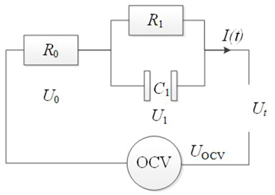
Figure 1.
The Thevenin model for a lithium-ion cell.
Here, OCV represents the open-circuit voltage Uocv; R0 represents the ohmic resistance; R1 and C1 in parallel represent the electrochemical reaction; I(t) is the current; Ut is the terminal voltage. The current-voltage behavior is then described as:
2.2. Parameters Identification
The OCV-SOC curve is obtained by averaging the charge and discharge curve of the rate of C/25 [21] at 25 °C, as shown in Figure 2. The OCV-SOC curve can be well fitted by a six-order polynomial, with an R-square of 0.998, given by:
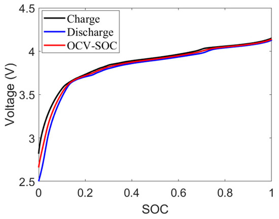
Figure 2.
OCV-SOC relationship.
Model parameters at different SOCs are estimated with the current step method, as shown in Figure 3a. The voltage profile in response to the current step at 80% SOC is shown in Figure 3b. The parameters R0, R1, and C1 are estimated in the voltage recovery process after interrupting the current. V0 represents the terminal voltage at the moment of interrupting the current, V1 represents the terminal voltage which is 2 s later than V0, and V2 represents the terminal voltage which is 60 s later than V1. R0 was calculated using:
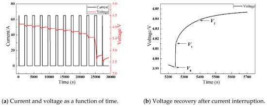
Figure 3.
Current step method for model parameterization.
R1 and C1 are estimated from fitting the voltage curve from V1 to V2 using a single exponential function, with coefficients related with R1 and C1 as follows [22]:
Figure 4 exhibits R1 and C1 as a function of SOC.
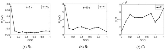
Figure 4.
Model parameters of the battery module as a function of SOC.
3. AHI Method, AEKF Method, and Alternate Method
In this section, we present a brief introduction of the AHI method, AEKF method, and the alternate method.
3.1. AHI Method
The AHI method is used widely as a practical solution in most battery management systems (BMS) [4,23], which is formulated as:
where represents the SOC at the initial time , QN is the rated capacity, denotes the coulombic efficiency, which equals to one and remains constant, represents the current which is, by definition, negative during charge and positive during discharge.
3.2. AEKF Method
The KF methods almost have higher estimation accuracies than the AHI method. Theoretically, all the KF methods can be used to combine with the AHI method composing the alternate method proposed in this paper. Among these KF methods and its improved forms, the AEKF and AUKF have higher estimation accuracy and better robustness because the noise covariance can be adjusted adaptively in the estimation process. For instance, Zhang et al. [23] proposed an AEKF method that reduced the estimation error to within ±2%. Furthermore, the AEKF method reduce the SOC estimation error from 20% to 1.5% within the first charge and discharge 40 s in our former work. Due to the AUKF and the AEKF methods having similar estimation algorithms, the AEKF method is chosen to combine with the AHI method to be the alternate method in this paper.
The AEKF [24] method uses as the state space, the current as the input, and the terminal voltage as the output of the system. Equations (1) and (5) are transformed to the following form:
The basic idea of the AEKF method is schematically shown in Figure 5.
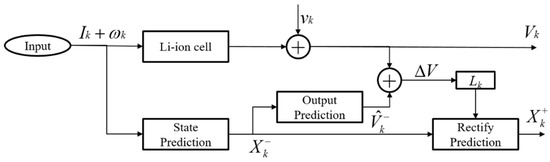
Figure 5.
State flow of the AEKF method for SOC estimation.
- Update the state and error covariance matrix at the step k by using the state and error covariance matrix at the step (k−1) (k = 2, 3 ...):
- Update the Kalman filter gain matrix calculation formula by:which corrects the SOC estimation and U1. The matrix of L(k) consists of the SOC-correction parameter Lks(k) and the U1 correction parameter Lku(k).
- Update the state and error covariance matrix at the step k with the output error by:
- The mean and covariance of the process noise and the observed noise are given by:
In Equations (6)–(10), Γ is an interference matrix, b represents a forgetting factor, , , q(k) and Q(k) represent the mean and covariance of the process noise, respectively, r(k) and R(k) represent the mean and covariance of the observed noise, respectively.
3.3. Alternate Method
To obtain high-precision SOC estimation at an acceptable cost, we propose an alternate method by combining the AHI method and the AEKF method. Figure 6 shows a detailed flowchart of the proposed method.
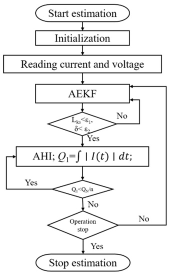
Figure 6.
Flowchart of the proposed approach for SOC estimation.
Firstly, the AEKF method is used to obtain an accurate initial estimation of SOC. When the switching condition of AEKF to AHI is satisfied, the alternate method switches to the AHI method. During the AHI period, the SOC estimation error increases due to the accumulation of the current-measurement error. Hence, when the absolute charge and discharge current integral capacity is larger than one-nth rated capacity the alternate method needs to switch back to the AEKF method to correct the SOC estimation error.
The switching conditions for the AEKF to AHI and the AHI to AEKF are explained below.
3.3.1. AEKF Switching to AHI
In this work, our experimental current and voltage data were collected using a high accuracy Maccor series 4000H which has a voltage acquisition accuracy of 1 mV and a current acquisition accuracy of 0.02 A. Considering the high acquisition accuracy of the equipment, the collected data are considered as true values. The true SOC value is calculated off-line using the AHI method. The SOC estimation error and SOC correction parameter Lks(k) in the AEKF method are shown in Figure 7, showing that the SOC estimation error is smaller than −3% and maintains between –3% and –1% when the SOC correction parameter Lks(k) converges to zero. If both absolute SOC correction Lks (ASCL) and the absolute deviation of SOC correction Lks at the adjacent estimation step (ADSCL) converge to zero, the SOC correction parameter Lks(k) will converge to zero. Therefore, and are chosen to be the threshold value of the ASCL and ADSCL, respectively, to make sure the AEKF method has obtain the accurate SOC estimation. Therefore, Equation (11) is used as the switching condition. It is important to identify the thresholds of the absolute SOC correction Lks (ASCL) and the absolute deviation of SOC correction Lks at the adjacent estimation step (ADSCL) as discussed in Figure 8.
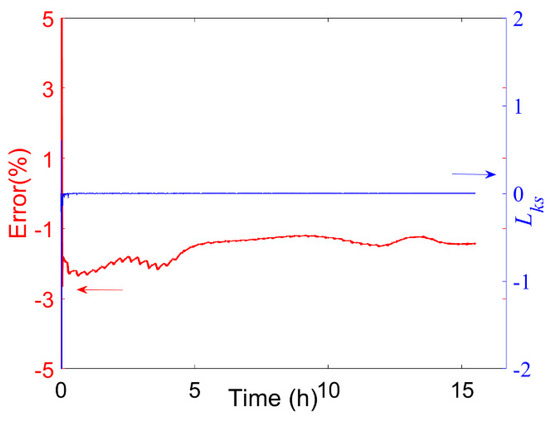
Figure 7.
SOC estimation error and Lks(k) in the process of SOC estimation by AEKF: the red line represents the SOC estimation error and the blue line represents the SOC correction parameter Lks.
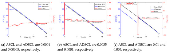
Figure 8.
SOC estimation process and errors using alternate method with ASCL and ADSCL of different values.
Here we should mention that when we study the alternate SOC estimation method using the collected current data, the AHI method will not introduce any error, which means the SOC error keeps constant in the estimation process using AHI method. Therefore, the stage of a constant SOC estimation error is the stage at which the AHI method works and the interval between two stages with different errors is where the AEKF method works. In Figure 8, the AHI and AEKF stages are marked with ellipse and rectangle, respectively. If the threshold for ASCL and ADSCL are too small ( is 0.0001, is 0.00005), the alternate method doesn’t involve the AHI method at all even though the AEKF method is already very accurate, as shown in Figure 8a. However, if the threshold values for ASCL and ADSCL are too large ( is 0.01, is 0.003), the alternate method will prematurely switch to the AHI method, as shown in Figure 8c. Figure 8b shows the alternate method which has suitable values of ASCL and ADSCL ( is 0.0035, is 0.0001). When the SOC estimation with the AEKF method becomes stable and accurate, it timely switches to the AHI method. Therefore, in this work, the threshold value of and are selected as 0.0035 and 0.0001, respectively.
3.3.2. AHI Switching to AEKF
The voltage and current collected by the high accurate equipment are considered as true value. To decide the switching condition from the AHI method to the AEKF method and to investigate the robustness of this alternate method, we factitiously add an amount of A mV to the voltage and multiple the current by 1 + B:
Equation (13) gives the SOC estimation error by the AHI method and it shows that the error has a linear relationship with the real charge or discharge capacity Qcd when the drift error of current is added. However, it is impossible to obtain the real charge or discharge capacity in the real operation. Nevertheless, Equations (12)–(14) show that the capacity Q1 which is calculated by the collected current with drift errors and the real capacity Qcd also have a linear relationship. Hence, Q1 is used to assess the switching condition. Besides, to obtain more accurate results, the capacity of Q2 which is calculated by the absolute value of charge or discharge current as shown in Equation (15) is chosen to replace the Q1, which makes it switch to the AEKF method earlier in the alternate method. Hence, Equation (15) is finally chosen to be the switching condition from the AHI method to the AEKF method. Q2 is compared with one-nth of QN (in this paper, n is integer value such as: n = 1,2,3…) to make sure that the AHI method switches to the AEKF method in time to avoid the absolute SOC error > 5%.
Here, SOCtrue represents the true SOC; SOCestimate represents the estimated SOC using the AHI method; SOCerror represents the estimated SOC error using the AHI method; SOCinitial-error represents the initial SOC error at the beginning of the AHI method; QN represents the nominal capacity of battery module; and Qcd represents the charged or discharged capacity in the process of SOC estimation, that is:
To assess the accuracy and robustness of these SOC estimation methods with voltage and current drift errors, the mean absolute error (MAE), maximum absolute error (MAXE), root mean square error (RMSE) and the standard deviation error (STDE) of the SOC estimation error are calculated as:
where is the SOC estimation result in each time step when the voltage or current contains drift error, and is the real value and N is the SOC estimated time steps. The range of [MAE-3*STDE, MAE+3*STDE] is chosen to inspect the switching conditions.
The suitable switching condition from AHI to AEKF is investigated with the voltage drift of +6 mV and current drift of −8% under the NEDC condition. Figure 9 shows the SOC estimation process and the corresponding estimation error under different switching conditions: n = 1 and n = 3. The SOC estimation error occasionally exceeds the error limit of 5% under the switching condition of n = 1. However, the SOC estimation error can be corrected effectively under the switching condition of n = 3. There exist two and five switches from AHI to AEKF for n = 1 and n = 3, respectively. The switching times from AHI to AEKF increases with n. Therefore, it is necessary to find the suitable value of n to guarantee the accuracy of SOC estimation and to shorten the process of SOC estimation using the AEKF method to reduce the computational burden. Figure 10 shows the MAE and the STDE of the SOC estimation error with different values of n. The results show that the MAE and the STDE decrease as n increases from 1 to 3. And when n is larger than 3, both MAE and STDE remain stable. Therefore, n = 3 is chosen as the suitable switching condition from AHI to AEKF.
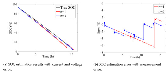
Figure 9.
SOC estimation with voltage drift of +6 mV and current drift of −8% under different transition conditions.
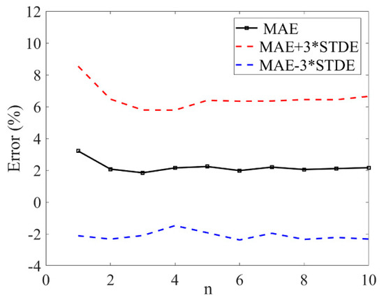
Figure 10.
MAE and the upper and down limitation as a function of switching number: n.
4. Experimental Results
To verify the proposed alternate method, NEDC experiments were performed in this work. Through the experiments, we also investigated the influence of current and voltage drift errors on SOC estimation results. Besides, we compared the accuracy, robustness, and real-time calculation ability of different estimation methods with varied drift errors. The battery module is composed of four cells in parallel, and the specifications of the battery module are listed in Table 1.

Table 1.
Cell specifications.
The collected current and voltage data of NEDC profile are shown in Figure 11, where negative current represents charge and positive current indicates discharge. The decreasing trend in the battery voltage indicates that discharge was the main process in the test. Note that all experiments were conducted in a thermal chamber at 25 °C.
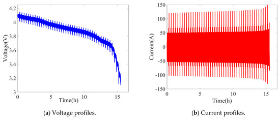
Figure 11.
NEDC profiles.
4.1. Influence of Current and Voltage Measurement Errors on SOC Estimation
Measurement errors can be ascribed mostly to the accuracy of the voltage and current sensors in BMS, and these errors manifest as drift or white noise added onto the true value. In this paper, the AEKF method are used to correct the initial SOC at the start and the SOC estimation error induced by the AHI method. Zheng et.al [25] found that the white noise has barely influence on SOC estimation results. Therefore, in this section, we only investigate the influence of current and voltage drift errors on SOC estimation using the AEKF method. The current and voltage drift errors are numerically introduced as shown in Equation (12). The current and voltage drift errors are shown in Table 2. Notice that the current is set as true when the voltage is added with different drift errors, and the voltage is set as true when the current is multiplied by different drift errors.
Table 2.
Voltage and current drift error.
Figure 12 shows the SOC estimation errors using the AEKF method with different drift levels of current and voltage. Figure 12a shows the influence of voltage drift on estimation error and Figure 12b shows the influence of current drift on estimation error. It can be seen that MAE almost has a linear relationship with voltage or current drift error. The upper and lower error boundaries increase with voltage and current drift errors. Figure 12 shows that if we want to limit the SOC estimation error within ±5%, the voltage and current drifts should be within −6.7~19.3 mV and −11.6~8.7%. Usually, the drift errors of the voltage and current measurement sensor in the BMS are symmetric [26]. Therefore, the voltage and current drift errors cannot exceed ± 6 mV and ± 8%, respectively.
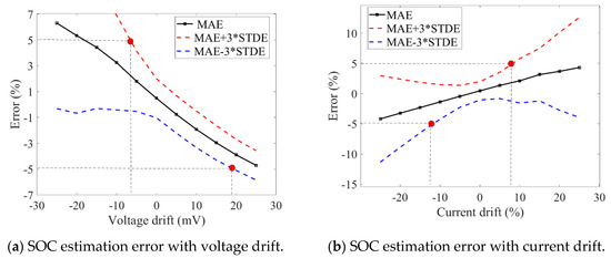
Figure 12.
SOC estimation error with voltage and current drifts.
4.2. Comparisons of Different SOC Estimation Methods under the NEDC Condition
In this part, the real initial SOC of battery module is set as 94%. The initial SOC for the AEKF method and alternate method is set as 80%, which is 14% away from the true value. However, the initial SOC for the AHI method is set as the true value (94%). The current and voltage drift errors are listed in Table 3.
Table 3.
Voltage and current drift errors.
Figure 13 shows the true SOC and estimation results and the corresponding estimation errors in the NEDC operation condition at 25 °C, respectively. The results show that the AEKF and alternate method can obtain accurate SOC estimation results in the whole operation even with inaccurate initial SOC and the current and voltage with ± 6 mV and ± 8% drift. In contrast, when the current is measured with drift errors, the SOC estimation errors of the AHI method grow in the process even with the true initial SOC value. The MAE, MAXE, RMSE, STDE, and the calculation time of the AEKF, the AHI, and the alternate method are shown in Table 4 with voltage drifts and current drifts as shown in Table 3. In addition, the calculation time is obtained by MATLAB software on a Thinkpad E450 PC produced by Lenovo, Beijing, China with Intel Core i7-5500U CPU produced by Intel, @2.40 GHz and 16.0 GB RAM.
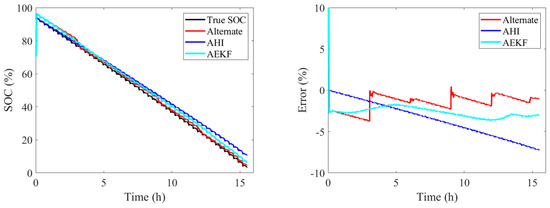
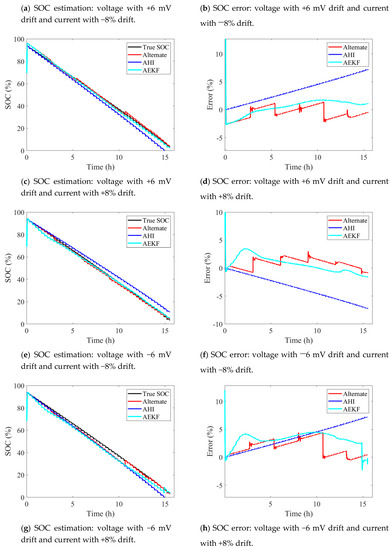
Figure 13.
SOC estimation results obtained using three methods.
Table 4.
SOC estimation errors and the time cost using different methods with voltage drifts and current drifts.
Table 4 shows that MAE, MAXE, RMSE, and STDE of the alternate method and AEKF method are almost same which means that the alternate method is as accurate as the AEKF method. However, these errors of AHI method are almost twice larger than the alternate method and AEKF method. Figure 13 shows that the SOC errors of AHI method is monotonic increased with the estimation steps when the current drift exists and the error increases from 0% to 7.2%. The error of AEKF method almost maintains in the range of −3% ~ 3% at the estimation group 1, 2, 3, and in the range of −5%~5% at the estimation group 4. The alternate method effectively correct the SOC error induced in the AHI method estimation process. Therefore, the SOC error of alternate method almost maintains same with the AEKF method. Meanwhile, the calculation times of the alternate method and the AHI method are almost same, and they are shorter than the AEKF method. The alternate method reduces the calculation load by about 75% compared to the AEKF method, which makes it possible in BMS to use the alternate method for every battery module’s real-time SOC estimation.
5. Conclusions
In this work, a new SOC estimation method combining the advantages of AHI and AEKF methods was proposed. The method was verified using a LMO-LNO battery module with a nominal capacity of 130 Ah. The experimental results indicate that the MAE, MAXE, RMSE, and STDE of the proposed alternate method and the AEKF method are almost the same. However, these errors of the AHI method are twice larger than the alternate method and the AEKF method. Therefore, the MAXE of the AHI method is 7.2% which exceeds predefined threshold even though the initial SOC is true. The alternate method effectively corrects the SOC estimation error induced by the current drift in the process of AHI estimation which prevent the SOC estimation error exceeding predefined threshold. As regards the computation cost, the proposed method, the AEKF method, and the AHI method cost 12 s, 49 s, and 10 s, respectively. In comparison, the proposed method achieves nearly the same estimation accuracy with the AEKF method at a calculation cost comparable with the AHI method.
Author Contributions
Data process: Z.L. (Zhongxiao Liu), Z.L. (Zhe Li), and H.G.; funding acquisition: Z.L. (Zhe Li) and J.Z.; methodology: Z.L. (Zhongxiao Liu), H.G., and Z.L. (Zhe Li); project administration: J.Z.; software: L.S. and Z.L. (Zhongxiao Liu); visualization: Z.L. (Zhongxiao Liu); writing—original draft: Z.L. (Zhongxiao Liu); writing—review and editing: H.G.
Acknowledgments
This research was funded by the National Natural Science Foundation of China under the contract of no. 51577104.
Conflicts of Interest
The authors declare no conflict of interest.
References
- Ren, G.; Ma, G.; Cong, N. Review of electrical energy storage system for vehicular applications. Renew. Sustain. Energy Rev. 2015, 41, 225–236. [Google Scholar] [CrossRef]
- Barré, A.; Deguilhem, B.; Grolleau, S.; Gérard, M.; Suard, F.; Riu, D. A review on lithium-ion battery ageing mechanisms and estimations for automotive applications. J. Power Sources 2013, 241, 680–689. [Google Scholar] [CrossRef]
- Steinhorst, S.; Shao, Z.; Chakraborty, S.; Kauer, M.; Li, S.; Lukasiewycz, M.; Narayanaswamy, S.; Rafique, M.U.; Wang, Q. Distributed reconfigurable battery system management architectures. In Proceedings of the 2016 21st Asia and South Pacific Design Automation Conference (ASP-DAC), Macao SAR, China, 25–28 January 2016; pp. 429–434. [Google Scholar]
- Lu, L.; Han, X.; Li, J.; Hua, J.; Ouyang, M. A review on the key issues for lithium-ion battery management in electric vehicles. J. Power Sources 2013, 226, 272–288. [Google Scholar] [CrossRef]
- Smith, K.A. Electrochemical control of lithium-ion batteries. IEEE Control Syst. Mag. 2010, 30, 18–25. [Google Scholar]
- Lotfi, N.; Fajri, P.; Novosad, S.; Savage, J.; Landers, R.; Ferdowsi, M. Development of an experimental testbed for research in lithium-ion battery management systems. Energies 2013, 6, 5231–5258. [Google Scholar] [CrossRef]
- Baccouche, I.; Jemmali, S.; Mlayah, A.; Manai, B.; Amara, N.E. Implementation of an Improved Coulomb-Counting Algorithm Based on a Piecewise SOC-OCV Relationship for SOC Estimation of Li-IonBattery. arXiv, 2018; arXiv:1803.10654. [Google Scholar]
- Einhorn, M.; Conte, F.V.; Kral, C.; Fleig, J. A method for online capacity estimation of lithium ion battery cells using the state of charge and the transferred charge. IEEE Trans. Ind. Appl. 2012, 48, 736–741. [Google Scholar] [CrossRef]
- Ng, K.S.; Moo, C.S.; Chen, Y.P.; Hsieh, Y.C. Enhanced coulomb counting method for estimating state-of-charge and state-of-health of lithium-ion batteries. Appl. Energy 2009, 86, 1506–1511. [Google Scholar] [CrossRef]
- Chaoui, H.; Ibe-Ekeocha, C.C. State of charge and state of health estimation for lithium batteries using recurrent neural networks. IEEE Trans. Veh. Technol. 2017, 66, 8773–8783. [Google Scholar] [CrossRef]
- Kim, T.; Qiao, W.; Qu, L. Real-time state of charge and electrical impedance estimation for lithium-ion batteries based on a hybrid battery model. In Proceedings of the 2013 Twenty-Eighth Annual IEEE Applied Power Electronics Conference and Exposition (APEC), Long Beach, CA, USA, 17–21 March 2013; pp. 563–568. [Google Scholar]
- Kim, I.S. Nonlinear state of charge estimator for hybrid electric vehicle battery. IEEE Trans. Power Electron. 2008, 23, 2027–2034. [Google Scholar]
- Charkhgard, M.; Farrokhi, M. State-of-charge estimation for lithium-ion batteries using neural networks and EKF. IEEE Trans. Ind. Electron. 2010, 57, 4178–4187. [Google Scholar] [CrossRef]
- Singh, P.; Vinjamuri, R.; Wang, X.; Reisner, D. Design and implementation of a fuzzy logic-based state-of-charge meter for Li-ion batteries used in portable defibrillators. J. Power Sources 2006, 162, 829–836. [Google Scholar] [CrossRef]
- Anton, J.C.; Nieto, P.J.; Viejo, C.B.; Vilán, J.A. Support vector machines used to estimate the battery state of charge. IEEE Trans. Power Electron. 2013, 28, 5919–5926. [Google Scholar] [CrossRef]
- Chen, C.; Xiong, R.; Shen, W. A lithium-ion battery-in-the-loop approach to test and validate multiscale dual h infinity filters for state-of-charge and capacity estimation. IEEE Trans. Power Electron. 2018, 33, 332–342. [Google Scholar] [CrossRef]
- Han, J.; Kim, D.; Sunwoo, M. State-of-charge estimation of lead-acid batteries using an adaptive extended Kalman filter. J. Power Sources 2009, 188, 606–612. [Google Scholar] [CrossRef]
- Aung, H.; Low, K.S.; Goh, S.T. State-of-charge estimation of lithium-ion battery using square root spherical unscented Kalman filter (Sqrt-UKFST) in nanosatellite. IEEE Trans. Power Electron. 2015, 30, 4774–4783. [Google Scholar] [CrossRef]
- Meng, J.; Luo, G.; Gao, F. Lithium polymer battery state-of-charge estimation based on adaptive unscented Kalman filter and support vector machine. IEEE Trans. Power Electron. 2016, 31, 2226–2238. [Google Scholar] [CrossRef]
- Hu, X.; Li, S.; Peng, H. A comparative study of equivalent circuit models for Li-ion batteries. J. Power Sources 2012, 198, 359–367. [Google Scholar] [CrossRef]
- Plett, G.L. Extended Kalman filtering for battery management systems of LiPB-based HEV battery packs: Part 2. Modeling and identification. J. Power Sources 2004, 134, 262–276. [Google Scholar] [CrossRef]
- Lu, J.X. Research on Characteristic Modeling and SOC Estimation of Lithium Ion Battery; South China University of Technology: Guangzhou, China, 2012; pp. 50–51. [Google Scholar]
- Li, Z.; Huang, J.; Liaw, B.Y.; Zhang, J. On state-of-charge determination for lithium-ion batteries. J. Power Sources 2017, 348, 281–301. [Google Scholar] [CrossRef]
- Zhang, Z.L.; Cheng, X.; Lu, Z.Y.; Gu, D.J. SOC estimation of lithium-ion batteries with AEKF and wavelet transform matrix. IEEE Trans. Power Electron. 2017, 32, 7626–7634. [Google Scholar] [CrossRef]
- Zheng, Y.J.; Xu, S.S.; Zhang, Z.D. Effect of sensor errors on state of charge estimation for ternary lithium-ion cells. J. Autom. Saf. Energy 2017, 8, 198–204. [Google Scholar]
- Available online: https://www.maximintegrated.com/en/landing/index.mvp?lpk=737 (accessed on 12 February 2019).
© 2019 by the authors. Licensee MDPI, Basel, Switzerland. This article is an open access article distributed under the terms and conditions of the Creative Commons Attribution (CC BY) license (http://creativecommons.org/licenses/by/4.0/).