Analysis of the Reduction of CO₂ Emissions in Urban Environments by Replacing Conventional City Buses by Electric Bus Fleets: Spain Case Study

Abstract

The emissions of CO₂ gas caused by transport in urban areas are increasingly serious, and the public transport sector plays a vital role in society, especially when considering the increased demands for mobility. New energy technologies in urban mobility are being introduced, as evidenced by the electric vehicle. We evaluated the positive environmental effects in terms of CO₂ emissions that would be produced by the replacement of conventional urban transport bus fleets by electric buses. The simulation of an electric urban bus conceptual model is presented as a case study. The model is validated using the speed and height profiles of the most representative route within the city of Madrid—the C1 line. We assumed that the vehicle fleet is charged using the electric grid at night, when energy demand is low, the cost of energy is low, and energy is produced with a large provision of renewable energy, principally wind power. For the results, we considered the percentage of fleet replacement and the Spanish electricity mix. The analysis shows that by gradually replacing the current fleet of buses by electric buses over 10 years (2020 to 2030), CO₂ emissions would be reduced by up to 92.6% compared to 2018 levels.

1. Introduction

Global warming continues to be one of the main problems the planet is facing, and transport is one of the most damaging sectors. According to reports by the International Energy Agency (IEA), in 2015, 32,250 MtCO₂ were emitted by combustible fuel throughout the planet (44.9% by coal, 34.6% by oil, 19.9% by gas, and 0.6% by other fuels [1]). Of these emissions, the transport sector is the second largest producer, contributing 24% of the total, only behind the electricity and heat sector, which contributes 42%.

Table 1. CO₂ emissions by transport sector (MtCO₂) [2,3,5,6].

Type of Transport	World (1990)	World (2015)	Spain 1990	Spain 2015
Road	3310 (72%)	5800 (75%)	51.26 (87%)	81.08 (94%)
International Marine Bunkers	380 (8%)	660 (9%)	-	-
Domestic Navigation	100 (2%)	180 (2%)	5.39 (9%)	1.99 (2%)
International Aviation Bunkers	260 (6%)	520 (7%)	-	-
Domestic Aviation	280 (6%)	320 (4%)	2.10 (3%)	2.70 (3%)
Other transport	280 (6%)	260 (3%)	0.45 (1%)	0.36 (1%)
Total (100%)	4610	7720	59.20	86.13

provides a breakdown of the various types of transport that contribute to CO₂ emissions, which clearly highlights road transport as the largest contributor, with 5800 MtCO₂ [2,3]. Road transport emissions cause two fundamental problems: (1) local order, since transport causes high levels of noise and pollution in urban areas (PM₁₀, PM_2.5, NOx, HC, CO), and (2) the global emissions of CO₂ into the atmosphere.

Despite the introduction of increasingly rigorous regulations aimed at controlling polluting emissions from conventional vehicles (powered by Internal Engine combustion (ICE) to diesel and gasoline), the underlying problem is the failure to consolidate already proposed policies to achieve a fundamental change in the use of alternative technologies. For example, the European Union (EU), looking at Horizon 2020, ruled on April 23, 2009 to implement the “DIRECTIVE 2009/28/EC OF THE EUROPEAN PARLIAMENT AND OF THE COUNCIL, on the promotion of the use of energy from renewable sources and amending and subsequently” [4], which makes reference to public transport, in particular, providing incentives for its use, the application of energy efficient technologies, and the use of renewable sources in the sector, in order to reduce the dependency on petroleum.

Analysing the subject at a local level (Spain), in 2013, 239.7 MtCO₂ were emitted by all sectors, and the largest CO₂-emitting sectors in Spain were transport (34.1%) and power generation (20.4%). Industry accounted for 16.6%, followed by other energy industries (including refining) producing 7.9%, households producing 6.6%, and the commercial sector producing 6.5% of the total [5]. The transport sector shows a similar trend at the world level, with road transport being the most representative in the contribution of CO₂, emitting 81.08 MtCO₂ of the 86.13 MtCO₂ total. In other words, this type of transport represents 94% of all the emissions of the sector.

The main cause of these high CO₂ emissions in the transport sector is the excessive use of energy vectors from non-renewable sources, especially gasoline and diesel. The problem of energy dependency is crucial in countries such as Spain that lack these resources, and are forced to import them. Therefore, it is essential to look for alternative sources and methods in order to reduce the demand for this type of resource.

Public transport via urban buses plays a fundamental role in society, as it is an efficient means to move a considerable number of people throughout a city. With the current occupation rate in relation to cars, a standard full urban bus could remove more than 40 cars from the city [7], which would considerably improve traffic problems, reduce noise pollution, improve air quality, and reduce pollution and greenhouse gas (GHG) emissions.

Considering society’s current mobility needs, the frequency of bus use has increased. As increasing the frequency increases the volume of the fleet, producing more emissions levels with conventional fleets. As such, a current theme is the promotion of sustainable mobility via various non-traditional solutions [8], where electric vehicles play a fundamental role. This type of vehicle has multiple advantages over conventional ICE powered vehicles such as no noise, no point of use emissions, high global performance, and principally not relying on petroleum.

Certain types of 100% electric powered urban buses are available on the market. They tend to have two configurations. The first consists of equipping the bus with a low capacity battery pack, compensated with high power. This type of configuration does not allow long journeys, and the vehicle needs to be recharged after just a few kilometres (between seven and 10 km). Its advantage is that charging only takes a few minutes and does not require a heavy large battery pack. However, its drawback is the need for an extensive infrastructure grid, which may incur high costs. The second configuration, which is analysed in this paper, involves equipping the bus with a large high-capacity battery pack [9], which allows travel for many kilometres. Once the working day is complete, it is charged, usually from the electric grid.

Currently, there are various original equipment manufacturers (OEMs) that produce electric buses solely powered using high-capacity batteries. Travel tends to be a minimum of 200 km, and Proterra (Proterra Inc., Burlingame, CA, USA) showcased a vehicle that can reach up to 563 km on one charge [10]. Consumption ratios tend to be between 0.9 and 1.8 kWh/km.

Table 2. Commercially available electric buses and their electrical power characteristics.

(OEM)	Model	Battery Capacity (kWh)	Range (km)	Energy Consumption (kWh/km)	Battery Technology
Proterra	Proterra Catalyst E2 [10]	440	404	1.09	Lithium-titanate
	Proterra Catalyst E2+ [10]	550	488	1.13
	Proterra Catalyst E2max [10]	660	563	1.17
BYD	BYD k7 [14]	195.6	217	0.90	Lithium-iron phosphate
	BYD k9s [15]	320	260	1.23
	BYD k9 [16]	324	250	1.29
	BYD k11 [17]	591	322	1.84
	BYD C6 [18]	128	200	0.64
	BYD C9 [19]	350	200	1.75
	BYD C10 [20]	394	322	1.22
Irizar	Irizar ie2 [21]	376	250	1.50	Sodium-nickel chloride
Designline	ECO-Smart I [22]	261.8	200	1.31	Sodium-nickel chloride
EBusco	YTP-1 [23]	311	300	1.04	Lithium-iron phosphate
Chongqing Hengtong	EBus [24]	77.6	50	1.55	Lithium-titanate
New Flyer	Xcelsior CHARGE [25]	454	418	1.09	Lithium-Ion nickel Manganese-cobalt
ZEPS	CCW ZEPS [26]	242	220	1.10	Lithium-iron phosphate

shows some models currently available on the market.

The estimated energy consumption during a driving cycle is highly important for these vehicles, as they operate in heavy traffic areas within the urban environment and have an extensive working day, meaning that the real travel distance can be less than claimed by the manufacturer. An example of this is the urban buses operating in Copenhagen, Denmark, where BYD k9 vehicles (BYD Auto, Shenzhen, Guangdong, China) were tested on different bus lines, with the results showing that, with heavy traffic, the consumption ratio varied between 1.24 and 1.77 kWh/km [11]. In other words, the autonomy is between 183 and 261 km for this vehicle, and the average error shows differences of up to 26.8% in relation to the manufacturer figures.

Simulation is a useful tool to estimate the energy consumed by an electric vehicle during a driving cycle. Prior studies, where electrically powered vehicle models have been implemented using AVL Cruise software (AVL, Graz, Austria), have proven this. For example, Varga [12] estimated the consumption of electric light-duty vehicles under the New European Driving Cycle (NEDC); the models used were the Citroen C-Zero, Mitsubishi i-MiEV, Renault Kangoo ZE, and Renault Fluence ZE. The results showed differences below 1.9% between the measured and simulated energy consumption. Another study was carried out by Rodrigues et al. [13] where they replaced a conventional taxi fleet by electric vehicles. The results showed that a light electric vehicle consumed up to eight times less energy than a petrol powered vehicle, with the advantages of not emitting CO₂, NOx, HC, CO, and suspended particles (PM_2.5, PM₁₀).

The electric vehicle concept consists of it being charged using the electric grid, meaning it is important to estimate the emissions they cause. The national energy matrix is one of the principal sectors involving a country’s social and economic development. Electric energy is an energy vector generated using primary resources (coal, oil, gas, wind, waste, solar, etc.), recorded in real-time from energy power stations. Electric power sources must have the following features: supply safety, quality, and diversification, so that its structure produces various types of electric power sources in order to minimize its impact on the environment. Furthermore, electric energy should allow economic competitiveness with suitable costs. Currently, there are important considerations and commitments in accordance with the Paris COP 21 [27] as well as the European Union energy strategy (2020 climate and energy package) [28], which aims to reduce greenhouse effect gas emissions with the aim of minimizing harmful changes to the planet.

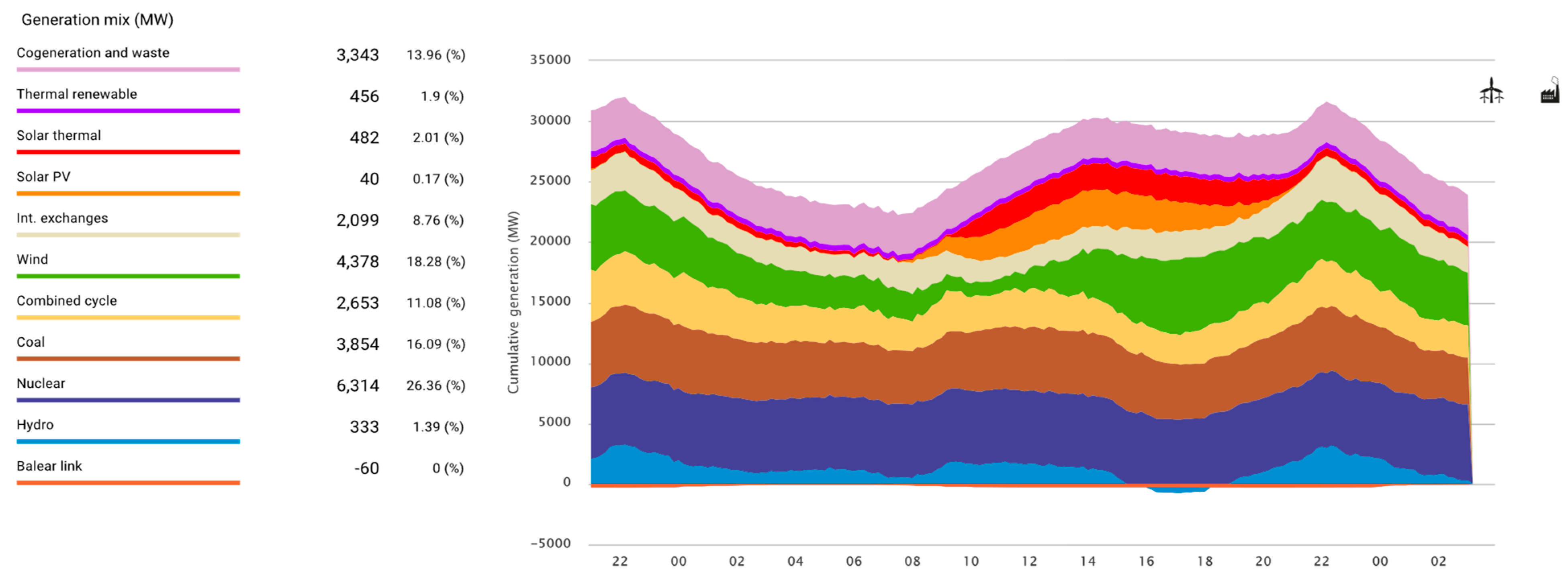
The Spanish electricity mix has electrical power stations including coal; fuel/gas combined cycle, which uses non-renewable resources (coal, natural gas, liquefied petroleum gas, petroleum, and derivatives); nuclear power stations (uranium-based); and electric power stations using renewable energy such as hydraulic, wind, photovoltaic solar (PV), thermal solar, biogas, and biomass. Renewable energies (excluding hydraulic that existed previously) have been implemented based on a legal framework that provided incentives for their introduction, with the aim was not being exclusively energy dependent on non-renewable sources.

Table 3. Electric power sources in Spain at the Iberian Peninsula [29,30].

Technology of Generator	Power (MW)	Electricity Generation (GWh)	Percentage of Contribution in Generation (%)
Renewable Energies
Wind	22,922	47,498	19.1
Hydroelectric	17,030	18,361	7.4
Solar PV	4439	7988	3.2
Solar Thermal	2304	5348	2.2
Other renewable	852	3603	1.5
Renewable waste	123	728	0.3
Total Renewable	47,670	83,526	33.7
Non-renewable Energies
Combined cycle (Gas)	24,948	33,855	13.6
Coal	9536	42,593	17.1
Nuclear	7117	55,609	22.4
Cogeneration CHP *	5818	28,134	11.3
Pumping	3329	2249	0.9
Non-renewable waste	459	2459	1.0
Total Non-renewable	51,207	164,898	66.3
Total	98,877	248,324	100

* Combined heat and power (CHP) plants.

shows the nominal installed power values for each type of power station and their electric energy contribution in 2017.

The Spanish electricity mix is quite diverse as there are 12 types of power station. This has occurred because Spain was one of the pioneers in the inclusion of alternatives energies in the national energy mix, with 104 GW total currently installed, of which 98.87 GW is produced on the Iberian Peninsula in Spain. The energy demand covered in 2017 was 248.4 TWh, of which 33.7% was met using renewable energies, whereas 66.3% was using conventional energy.

A controversial issue related to electric vehicles is the life cycle of batteries and how it affects CO₂ emission intensity. The battery lifespan leads to comparison with several technologies, mainly diesel and petrol vehicles. Studies in which the complete life cycle of an electric vehicle has been analysed showed that contamination by lithium batteries is only 13% of the vehicle’s total CO₂ emission intensity [31].

A strength of the electric vehicle in comparison to traditional technologies is that it depends the electricity mix of a country. In the European Union, the Polish have the highest emission factor (650 g CO₂/kWh). Despite this, if electric vehicles are incorporated into this electricity mix, their CO₂ emission intensity is 25% less polluting than a light diesel vehicle. As the average emission factor is 300 g CO₂/kWh, the European Union goal to reach 200 g CO₂/kWh by 2030 further supports the use of electric vehicles.

Having viewed the current situation in relation to electric vehicles and its application in urban buses, this paper aims to characterise, via simulation, a conceptual model with this type of powertrain. The parameters and specifications are set to those determined for this type of vehicle. To estimate the energetic behaviour, the city of Madrid urban route is used as a reference, specifically the C1 circular line, which is considered as the most representative. The company charged with managing this transport is Madrid Municipal Transport Company (EMT), which has 2050 buses and 209 routes. Its importance in the city`s transport system is so significant that it carried 430 million passengers in 2016 [32].

The proposed approach for an urban bus with a large high-capacity battery pack is based on EMT’s intent to gradually electrify its fleet (strategic plan 2017–2020 [33]), where 15 electric buses with characteristics like the proposed conceptual model have recently been acquired. The current percentage of the fleet with vehicles of this type is 1.76%, corresponding to 36 units.

The electric urban bus completes a traditional working day (16–18 h), then the electric energy consumed is recharged to complete a new working day. As a conceptual framework, this type of vehicle should be charged using the electric grid, so that the search for primary energy sustainability can be recommended. The current Spanish electricity mix has a representative contribution of renewable energies and the night time is a good time for the vehicles to be connected to the electric system.

The final part of this paper considers the gradual replacement of the fleet and its effect on the reduction of CO₂ emissions.

2. Methodology

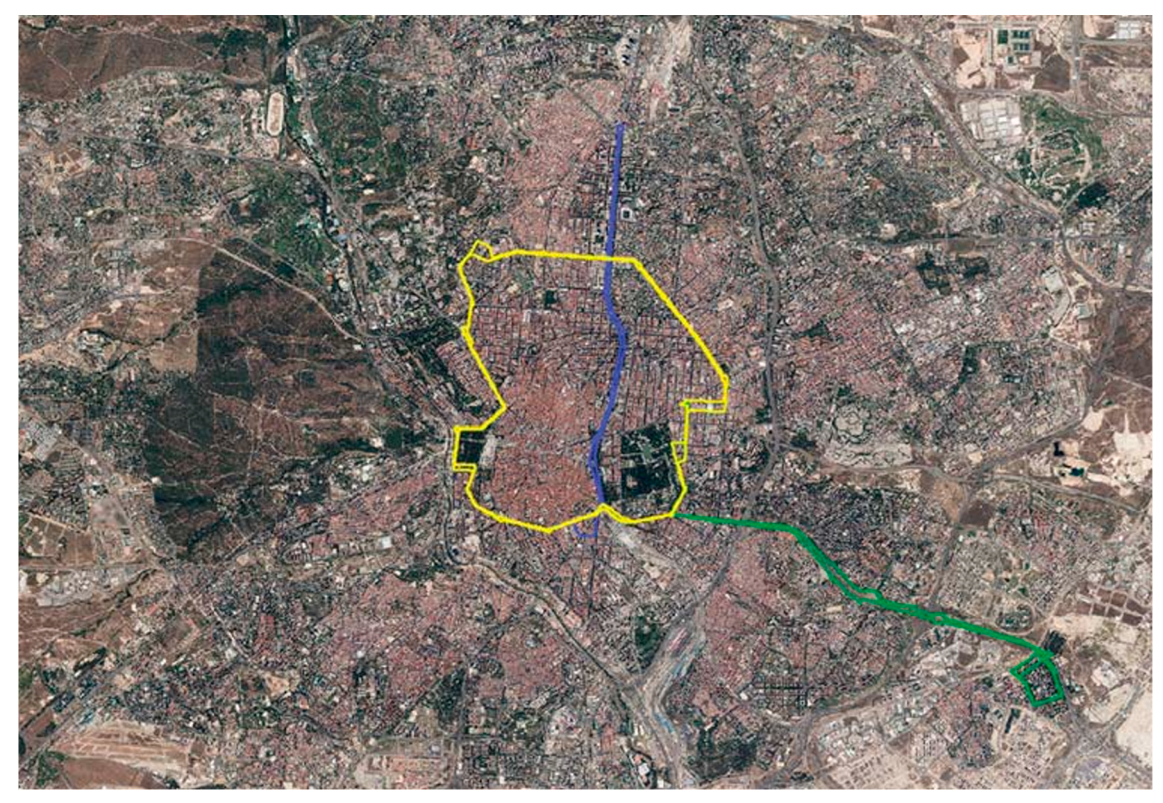
Experimental data obtained from real drive conditions were used as a starting point. These routes were selected from the three most significant clusters; the routes correspond to the 27, 63, and C1 (Figure 1) bus lines in the city of Madrid [34], which were chosen because they resemble 53% of bus routes in the urban area that circulate in Madrid. Our work is based on previous studies [34,35,36,37,38] developed by the University Institute for Automobile Research, Technical University of Madrid (INSIA) and applied to the EMT bus fleet, where 30 lines were tested using on-board equipment. These conditions allowed us to mimic reality, including all sources of variability, such as environmental conditions and traffic, driver behaviour, highly transitory operation, and the variable operating conditions of the vehicles.

The measurements were recorded when the bus was in service; movement cycles and stop periods can be distinguished and these periods are called kinematic micro-cycles. The movement cycles are characterised by variables such as total time, constant speed times, acceleration and deceleration process times, and average acceleration and deceleration times.

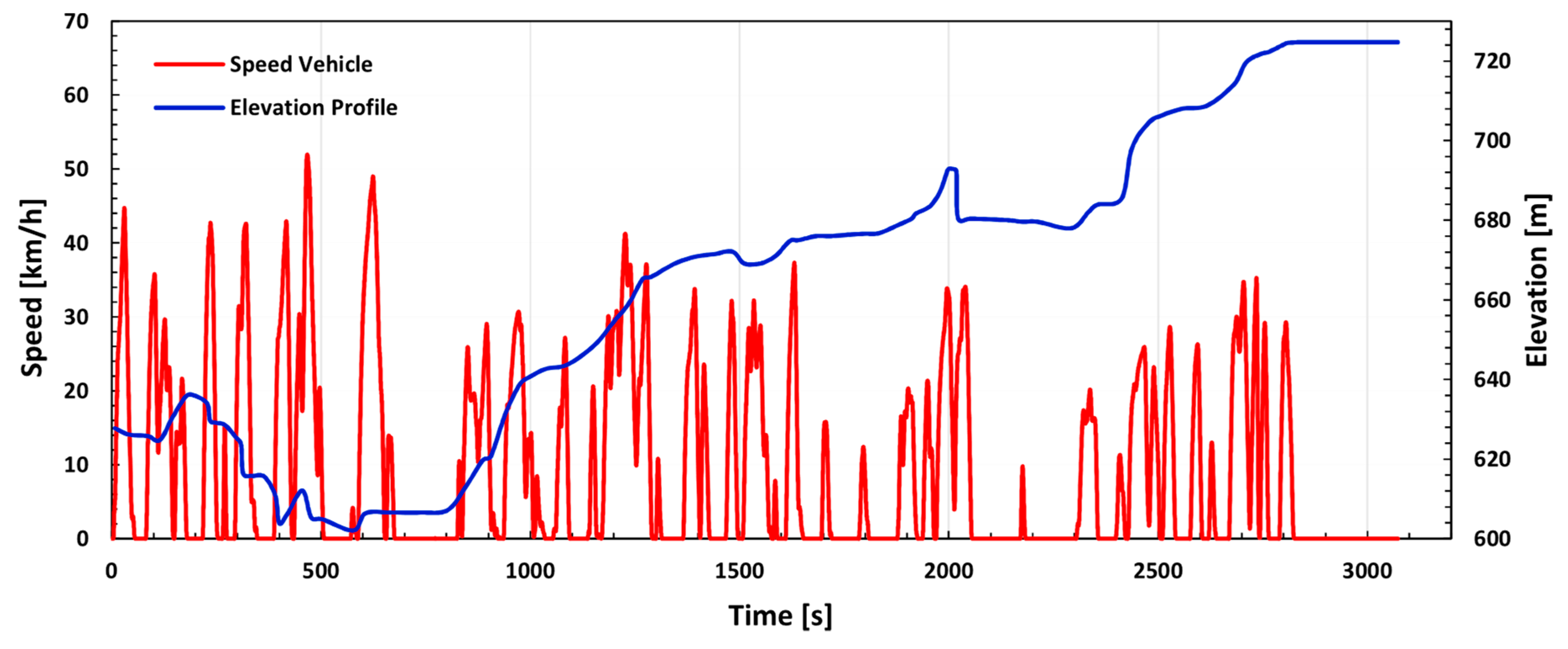
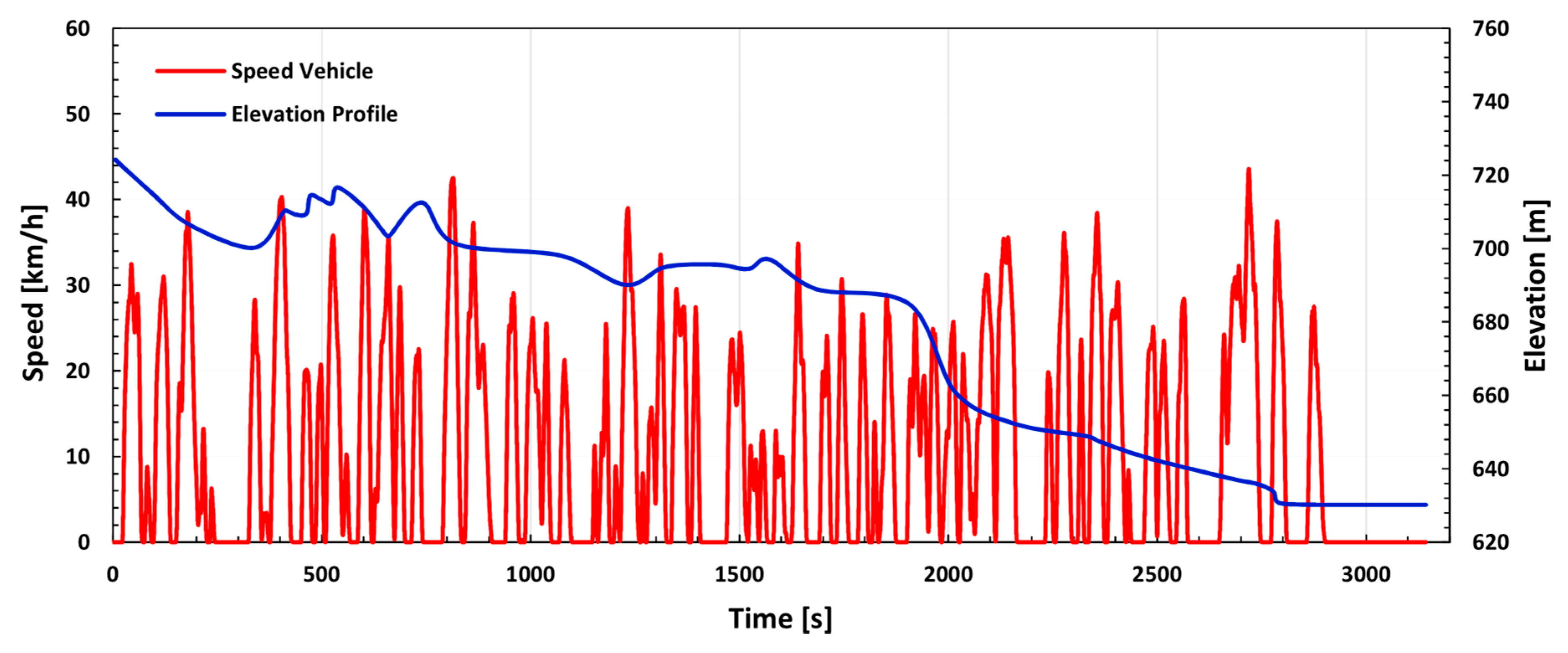
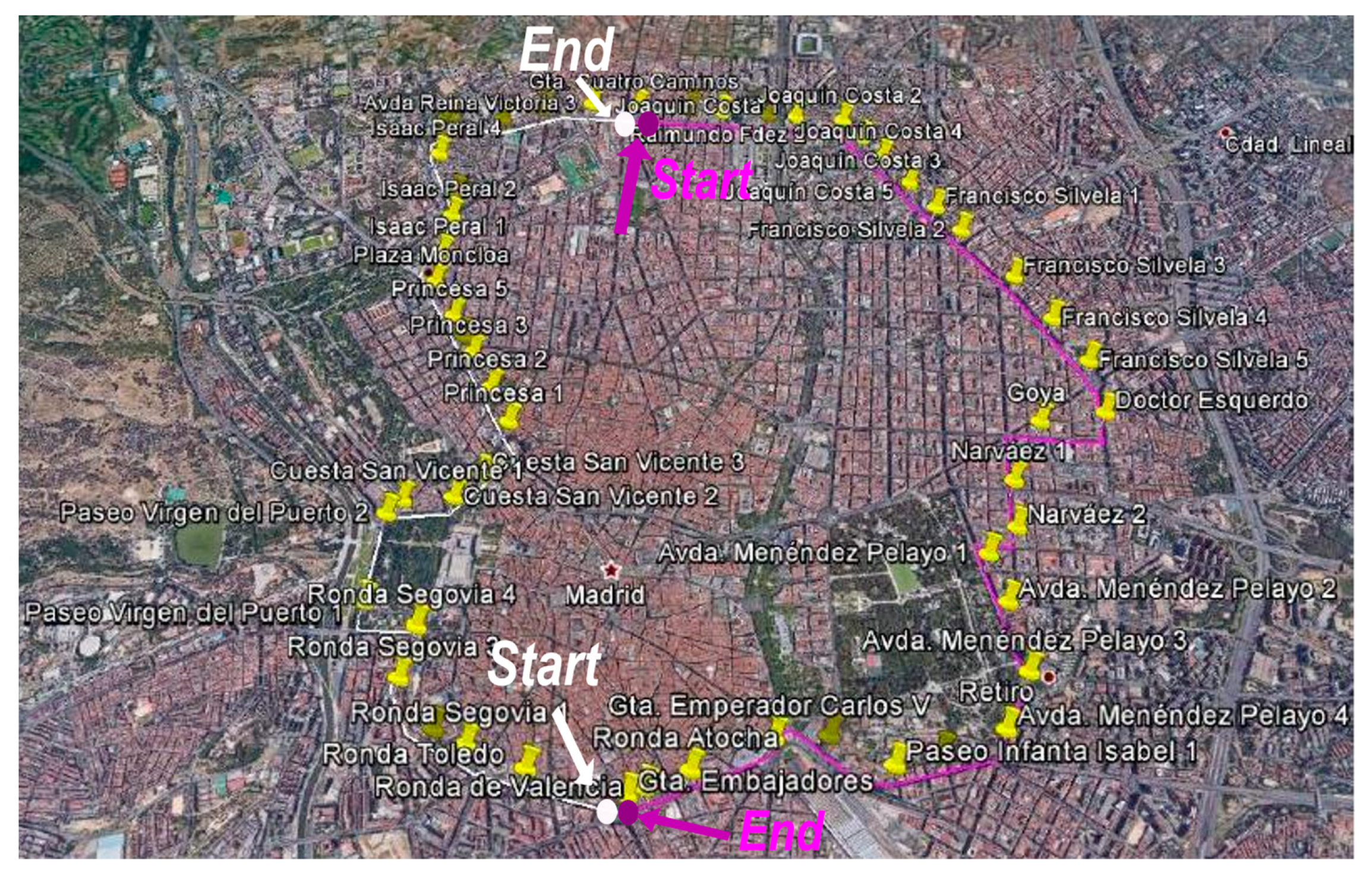
The data obtained from the C1 circular line (Figure 2) were chosen and the speed and height profile are depicted in Figure 3 and Figure 4, respectively. This driving cycle is variable and best represents the different operational conditions within the city’s urban environment. The route was divided into an outgoing itinerary (route 1) and an incoming itinerary (route 2).

Table 4. Specifications of the measured driving cycle.

Route	Maximum Speed (km/h)	Average Speed (km/h)	Distance (km)	Time (s)	Number of Stops
1	51.94	10.36	8.12	3073	30
2	44.82	11.66	9.40	3143	26

provides a summary of the data obtained from the trials.

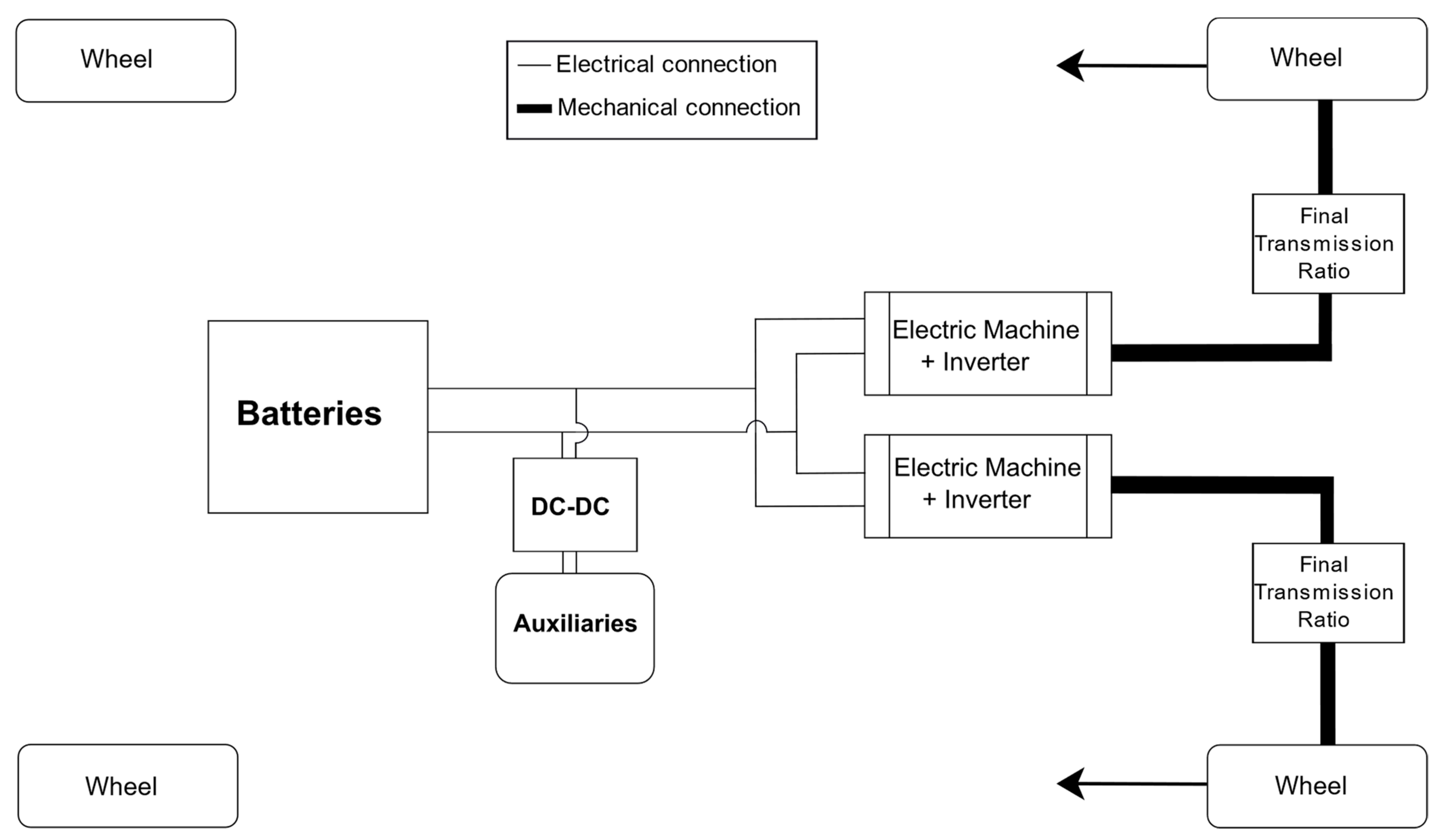
2.1. Design of the Propulsion System

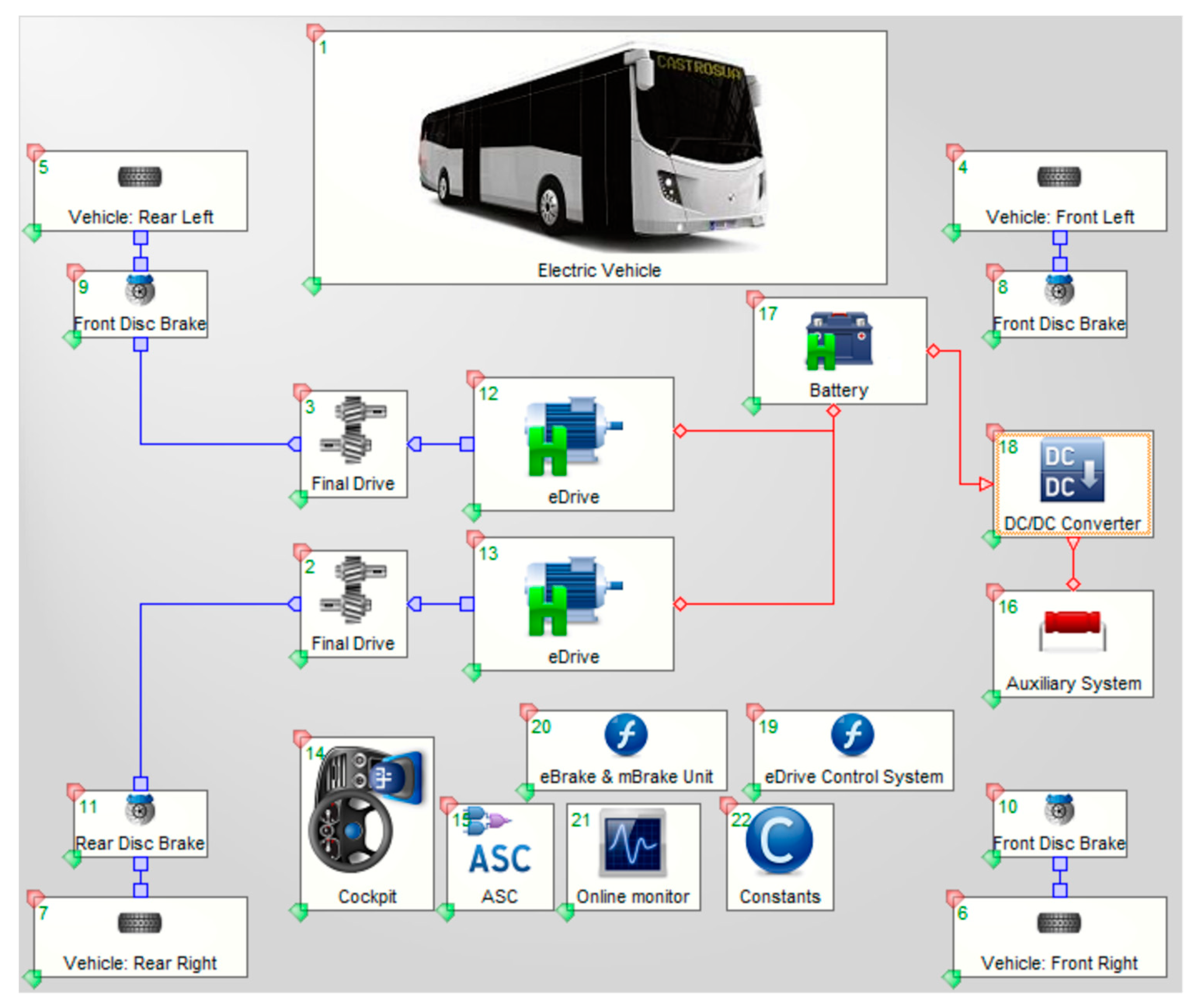
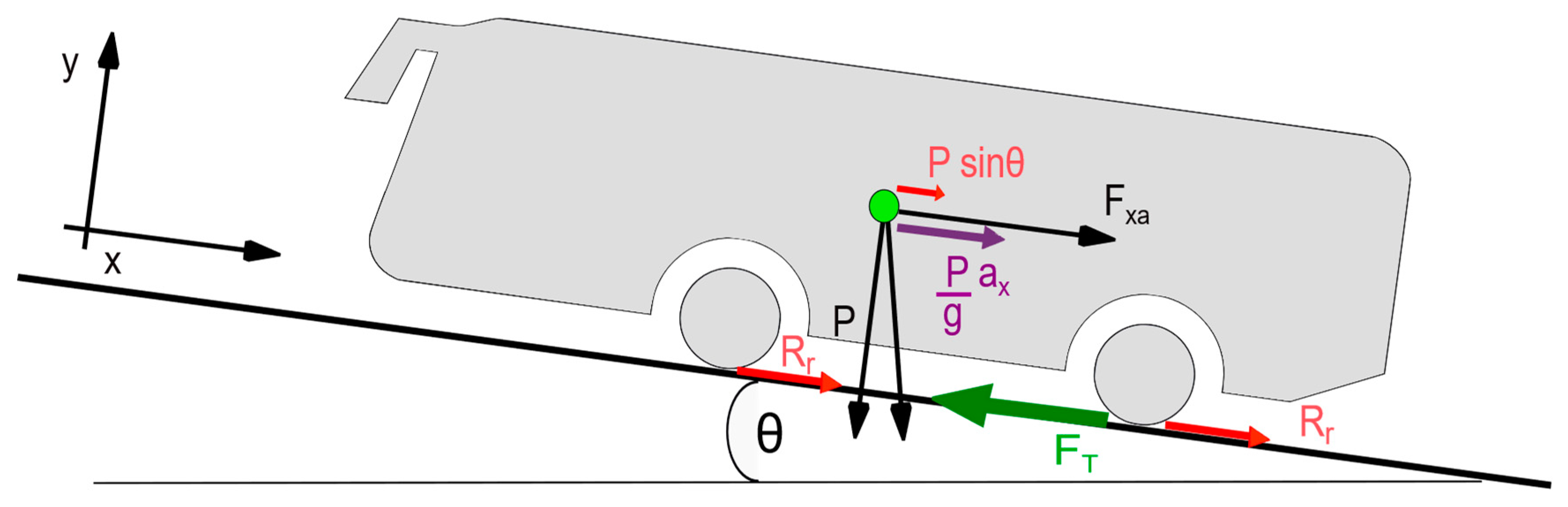
The configuration of the system is shown in Figure 5. The powertrain was composed of: energy storage unit or batteries, electric machines, DC–DC converters, DC–AC inverter, auxiliary systems, and final transmission ratio. The optimal design of the powertrain depends, to a large extent, on the correct analysis of the longitudinal vehicular dynamics [39,40]. To calculate the tractive effort necessary for the movement of the vehicle, the resistant forces that must overcome were analysed (Figure 6), including: rolling resistance, aerodynamic drag, gravitational resistance, and resistance to inertia. Applying Newton’s second law and the Euler equation, we have:

$$m{a}_x{\gamma }_m=F_T-R_r-F_{xa}-R_g$$

(1)

where m is gross mass, $a_x$ is longitudinal acceleration, ${\gamma }_m$ is the mass factor, $F_T$ is the tractive effort developed by a traction motor on driven wheels, $R_r$ is rolling resistance, $F_{xa}$ is aerodynamic drag, and $R_g$ is gravitational resistance.

So, the tractive effort is equal to:

$$F_T=m{a}_x{\gamma }_m+R_r+F_{xa}+R_g$$

(2)

${\gamma }_m$ is estimated by the following expression:

$${\gamma }_m=1+{{\displaystyle \sum }}^{\text{}}\frac{I_r}{m{r}^2}+{{\displaystyle \sum }}^{\text{}}\frac{I_t{\mathsf{\xi }}_j^2}{m{r}^2}$$

(3)

where $I_r$ is the moment of inertia of the masses that turn with the wheels with respect to their rotary axes, $I_t$ is the moment of inertia of the transmission components, $r$ is the kinematic radius equivalent to the radius of the wheel under a load, and ${\mathsf{\xi }}_j$ is the final transmission ratio.

Alternatively, the tractive effort $(F_T)$ can be calculated once the powertrain has been dimensioned through the following expression:

$$F_T=\frac{M_{ME}{\xi }_j{\eta }_j}{r_e}$$

(4)

where $M_{ME}$ is the moment of inertia of the masses that turn with the wheels with respect to their rotary axes, ${\eta }_j$ is the moment of inertia of the transmission components, and $r_e$ is the radius under load (effective radius of the driven wheels).

2.1.1. Performance criterion

For heavy vehicle applications, particularly in relation to human transport in urban environments, we complied with the following general and specific conditions for this study case:

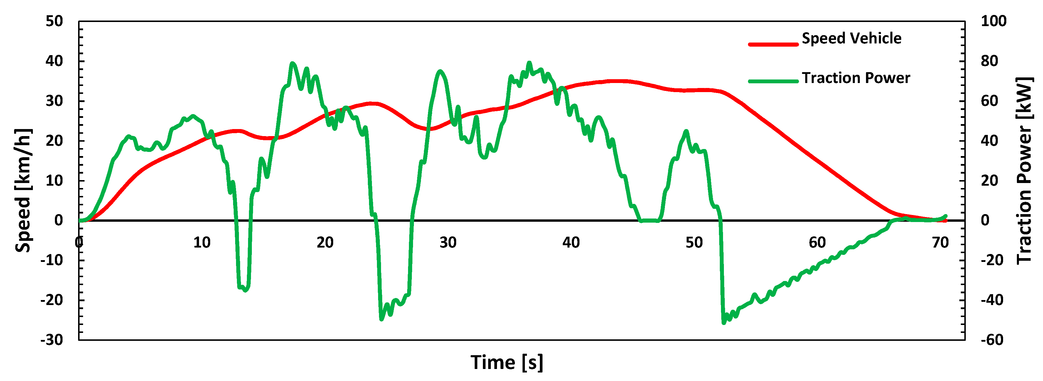
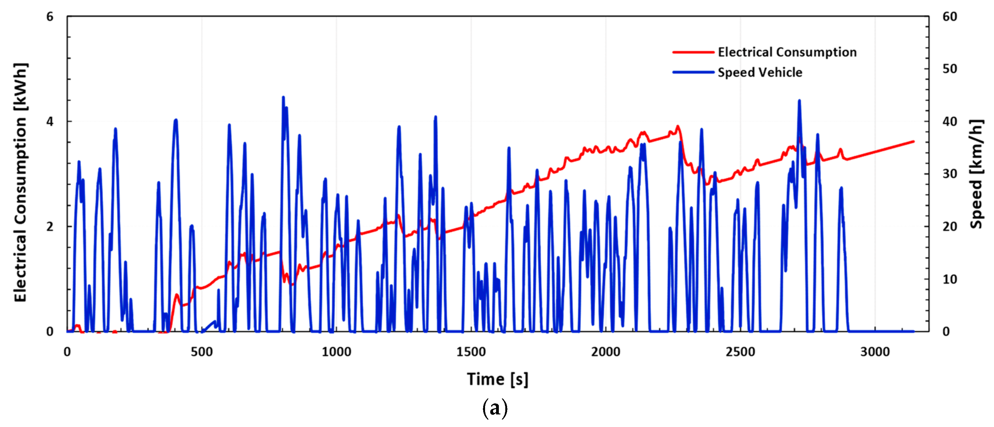
• The drive cycles are normally repeated using the same pattern: cycles between one and three minutes as a maximum, with speeds below 60 km/h (Figure 7).
• Numerous stops are used that reduce the average power used during traction; however, there is an increase in the number of accelerations and decelerations.
• There are high autonomy needs given that the service duration tends to be around 18 h, the working day is from 5:30 a.m. to 11:30 p.m., meaning the window of connection to the electric grid is limited to between 12:30 and 4:30 a.m., considering time losses due to logistics.
• There is high energy consumption from auxiliary systems, so when sizing the energy storage system, attention should be paid to this variable.

Performance criteria are limited to the speed requirements in urban areas, where buses rarely reach speeds of 60 km/h given the short distances between stops, as well as other factors such heavy traffic and speed restrictions. The criteria that were considered when designing the powertrain were: maximum speed, acceleration, and maximum slope [41,42,43].

Table 5. Specifications of the electric urban bus.

Specification	Value	Specification	Value
Vehicle mass (mv)	13,800 kg	Maximum slope ($\theta$)	18%
Maximum Authorized Mass (mmax)	18,000 kg	Maximum speed ($v_{max}$)	65 km/h
Rate load (mPAS) (32 seated and 20 standing of 70 kg)	3640 kg	Base Speed ($v_b$)	15 km/h
Frontal area ($A_f$)	7.2 m2	Nominal radius of the driven wheels ($\mathrm{r}$)	0.571 m
Aerodynamic drag coefficient ($C_x$)	0.6	Acceleration time from 0 to 65 km/h ($t_a$)	28 s
Air density ($\rho$)	1.225 kg/m3	Drivetrain efficiency (${\eta }_j$)	96%
Gravity acceleration ($g$)	9.81 m/s2	Final transmission ratio (${\xi }_j$)	17.7
Rolling resistance coefficient ($f_r$)	0.012	Combined efficiency of the E.M (ηME) and the inverter DC–AC (ηDC–AC)	90%
Mass factor (${\gamma }_m$)	1.04	Efficiency of the DC–DC converter (ηDC–DC)	95%

shows the urban bus conceptual model specifications.

The power can be estimated under the aforementioned criteria. The tractive power required for the maximum speed is determined using the following equation:

$$P_{t_{vel}}=\left[\left(mg{f}_r\right)+\left(\frac{1}{2}\rho C_x{A}_f{v}_{m\mathrm{a}x}^2\right)\right]v_{m\mathrm{a}x}$$

(5)

where $P_{t_{vel}}$ is the tractive power for the maximum speed, $g$ is the gravity acceleration, $f_r$ is the rolling resistance coefficient, $C_x$ is the aerodynamic drag coefficient, $\rho$ is the air density, $A_f$ is the frontal area, and $v_{max}$ is the maximum speed.

The tractive power required for acceleration is considered the acceleration time from zero up to a specified speed (65 km/h). Equation (6) states this as:

$$P_{t_{ace}}=\frac{{\gamma }_{m}m}{2t_a}\left(v_f^2+v_b^2\right)+\frac{2}{3}mg{f}_r{v}_f+\frac{1}{5}\rho C_x{A}_f{V}_f^3$$

(6)

The tractive power required for acceleration ($P_{t_{ace}}$) in this equation is applied to a specific acceleration standard, where $t_a$ is the acceleration time employed, which is 28 s in this case. $t_a$ is defined based on how long it takes the vehicle to reach its maximum speed from its initial speed equal to 0 km/h. $v_b$ is the base speed of the vehicle (15 km/h) and $v_f$ is the final speed (65 km/h) and is the maximum speed of the vehicle.

For the tractive power required for a maximum slope (18%), the speed at which this section is travelled (15 km/h) is considered. In this case, the aerodynamic resistance can be ignored as the progress along elevated inclines occurs at reduced speeds. The equation is set as:

$$P_{t_{slp}}=\left(mg{f}_r\cos \theta mg\sin \theta \right)V_b$$

(7)

where θ is the angle of the slope to be overcome and $V_b$ is the speed the bus must travel to overcome the slope (base speed in this application). The results show that the tractive power required for maximum speed ($P_{t_{vel}}$) is 52 kW for an acceleration ($P_{t_{ace}}$) of 142 kW and for a maximum slope ($P_{t_{slp}}$) of 132 kW.

2.1.2. Vehicle Transmission

The vehicle transmission regulates the transfer of power (torque and speed) from the electric machine to the wheels. For this, a gear system is normally used, and for electric vehicles, a single gear change may be necessary. However, this depends on the torque and speed of the vehicle. If the constant power range is large, it may provide enough high torque at low revolutions; otherwise, a multiple gearbox should be used.

The size of the electric machine in nominal power terms is linked to the mechanical power and efficiency. These are obtained based on the nominal efficiency minimum requirements, which should comply with IE2 efficiency levels as of June 16, 2011 in accordance with the European Commission [44]. The efficiency for this type of motor is around 94%. The following equation determines the electric power of the machine:

$$P_{EM{,}_{el}}=\frac{P_{E{M}_{mec}}}{{\eta }_{EM}}$$

(8)

$$P_{E{M}_{mec}}=\frac{P_{t_{ace}}}{{\eta }_j}$$

(9)

where $P_{EM{,}_{el}}$ is the electrical power, $P_{E{M}_{mec}}$ is the mechanical power, ${\eta }_{EM}$ is the efficiency of the electric machine, $P_{t_{ace}}$ is the tractive power required for acceleration, and ${\eta }_j$ is the drivetrain efficiency.

The maximum motor torque characteristic is described via the correlations between the output torque, the output power, and the angular speed. The motor output torque is calculated using the following expression:

$$M_{E{M}_{out}}=\frac{P_{E{M}_{mec}}}{{\omega }_{EM}}$$

(10)

$${\omega }_{EM}={\xi }_j{\omega }_{re}={\xi }_j\frac{V_{re}}{r_e}$$

(11)

$$r_e=r\left(1-i\right)$$

(12)

where $M_{E{M}_{out}}$ is the output torque, ${\omega }_{EM}$ is the angular motor speed, ${\xi }_j$ is the final transmission ratio, ${\omega }_{re}$ is the angular speed of the wheel, $V_{re}$ is the linear vehicle speed, $\mathrm{r}$ is the nominal radius of the driven wheels, and $\mathrm{i}$ is the longitudinal sliding (0.1–0.3).

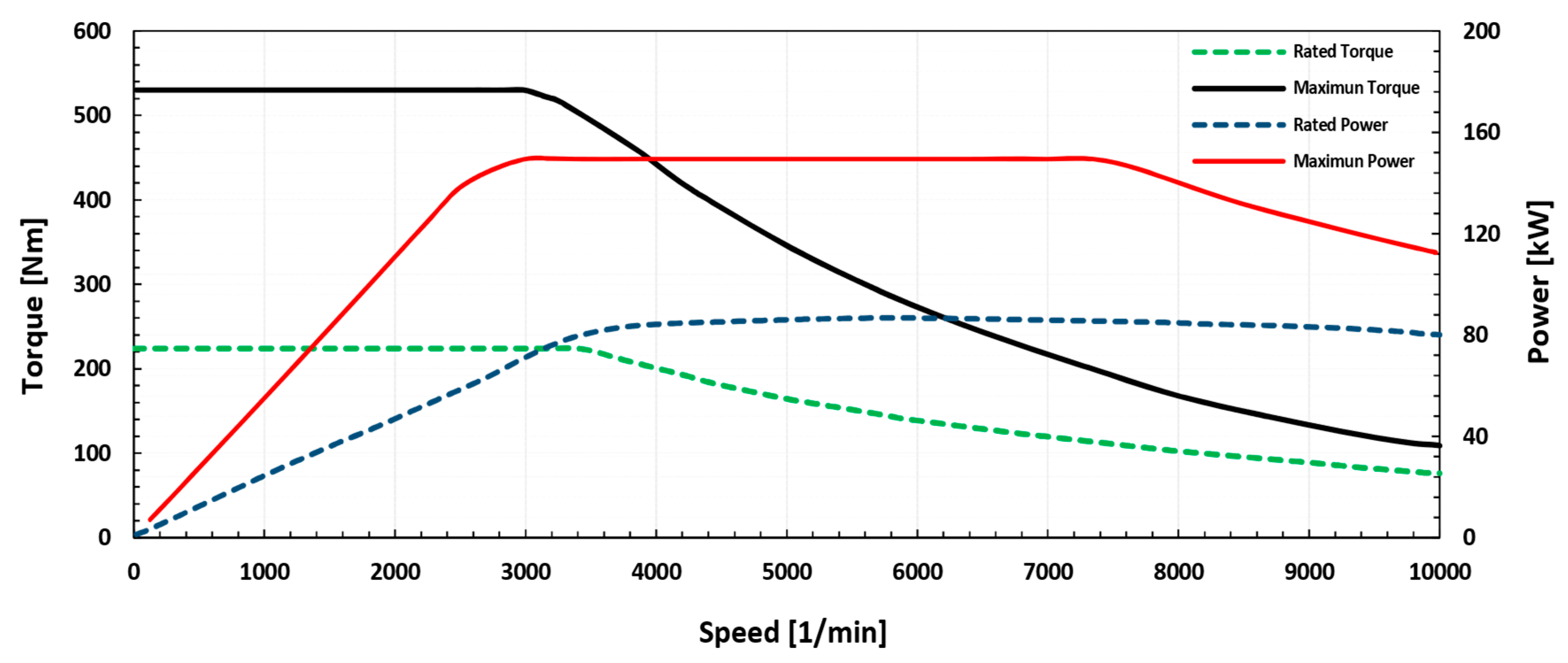
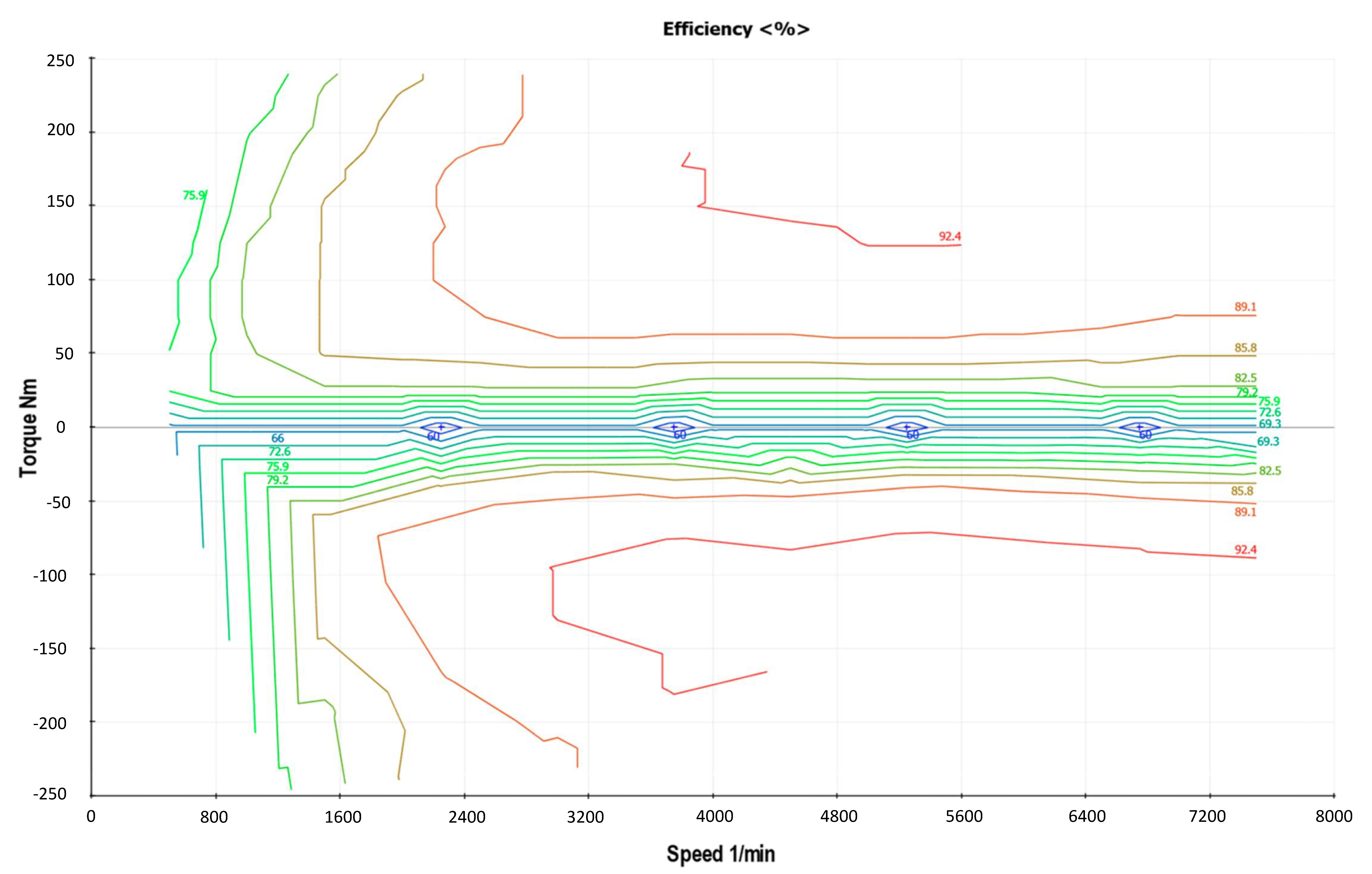
The above calculations determine that the electric machine power should be around 157 kW and the required torque should be 152 Nm. To complete the simulation, the characteristics of two motors connected to each rear wheel were chosen. The nominal power of each was 85 kW with a nominal torque of 220 Nm. The total nominal power was 170 kW and 440 Nm total nominal torque. The characteristic curve of this motor can be seen in Figure 8, where the torque and maximum power are 530 Nm and 150 kW, respectively, for each motor, which cover the full range of requirements.

Table 6. Specifications of the electric machine [45].

Specification	Value	Specification	Value
Rated Voltage	650 V	Rated Current	142 A
Rated Power	85 kW	Maximum Speed	10,000 Rpm
Rated Torque	220 Nm	Weight	120 kg
Maximum Torque	530 Nm	Dimension	510 × 245 × 245 mm
Maximum Power	150 kW	Ambient temperature	−30 to 70 °C

shows the details of the characteristics of this component.

2.1.3. Auxiliary System

The energy consumption estimates for the auxiliary components (interior and exterior lighting, refrigeration pump, electrical steering, air conditioning, pneumatic brakes) are of great importance because the vehicle energy is limited, and recharging can take a long time. As the vehicle is in constant operation throughout the day, the energy consumption of the auxiliary systems may be high, from 20 to 40 kWh/100 km for this type of vehicle according to the IEA [46].

Gao et al. estimated the energy consumption of the auxiliary systems as 3980.2 kJ and 4812.1 kJ (1.1 kWh and 1.33 kWh, respectively) for two different types of powertrains for urban routes in China according to the China Typical Bus Driving Cycle CTBDC), which has an approximate time of 1300 s. However, during these tests, operation of air-conditioning was not included [47,48].

According to Miranda et al., the instant peak power of all the auxiliary systems together did not exceed 10 kW on an 11-km-long urban bus route in Brazil. The vehicle consumed 17.6 kWh of net energy with the auxiliary systems consuming 2.46 kWh for 1250 s during the route. These values represented 14% of the total energy consumption of the system, with a total consumption ratio of the vehicle of 1.6 kWh/km [49].

Gao et al. estimated the power of auxiliary systems on series and parallel hybrid buses as being 2.29 kW [50], with 3.75 kW for electric buses [51], as opposed to Göhlich et al., who found power consumption of 6 kW for the auxiliary systems [52].

Based on the literature, a value of 5 kW of power is proposed for the auxiliary systems. For the model to be more accurate, we decided that the power will be constant during the full journey, so that it will represent extreme energy consumption in the simulation model.

2.1.4. Battery Model

The battery power should be in excess or equal to the electric machine’s power ($P_{EM}$) plus the auxiliary system’s power $(P_{aux}),$ meaning the battery power should be at least 175 kW. The following equation estimates the above:

$$P_{BAT}\ge P_{EM}+P_{aux}$$

(13)

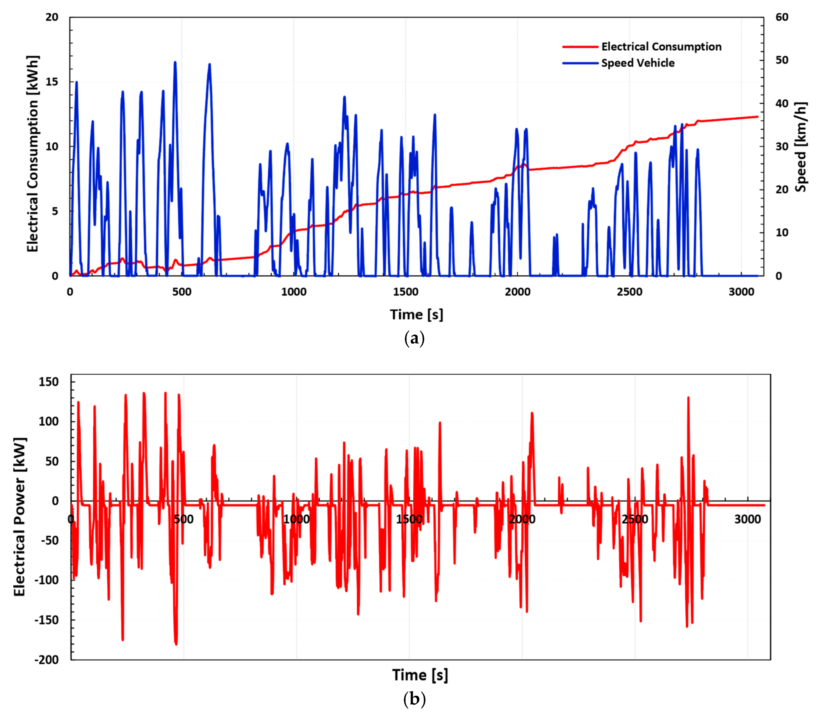
The output power on the battery terminals during the running of the routes is calculated using the following equation:

$$P_{BAT{,}_{out}}=\frac{V}{{\eta }_{EM}{\eta }_j}\left[mg{f}_r+mg\sin \theta +\frac{1}{2}\rho C_x{A}_f{V}^2+m{a}_x{\gamma }_m\right]+P_{aux}$$

(14)

The first term represents the power necessary for traction, which is equal to the resistance power over the loss of power in transmission and the electric machine, represented by their efficiencies ${\eta }_j$ and ${\eta }_{EM}$, respectively. The second term represents the power of consumption of the auxiliary components, which is considered constant in this model. The regenerative braking power during the driving cycle at the battery terminals can be expressed as:

$$P_{BAT{,}_{in}}=\frac{\lambda V}{{\eta }_{EM}{\eta }_j}\left[mg{f}_r+mg\sin \theta +\frac{1}{2}\rho C_x{A}_f{V}^2+m{a}_x{\gamma }_m\right]$$

(15)

where the slope, acceleration, or even both are negative; $\lambda$ ($0<\lambda <1$) it is the regenerative braking factor, which is an applied braking effort function of the design and control of the braking system in a way that allows the estimate of the braking percentage to be recovered when using the electric machine.

The energy supplied by the battery during the driving cycle is determined using the following equation:

$$E_{BAT}={{\displaystyle \int }}_{t_0}^{t_1}{P}_{BAT{,}_{out}}dt-{{\displaystyle \int }}_{t_0}^{t_1}{P}_{BAT{,}_{in}}dt$$

(16)

The first term represents the energy necessary for traction and the energy consumed by the auxiliary systems, whereas the second term is the energy recovered by the regenerative braking effect. For the analysis of this model, a battery capacity of 324 kW was determined, which is within an acceptable range for this type of vehicle (Table 2).

Lithium-iron phosphate batteries were proposed during the design. The energy density oscillates between 80 and 130 Wh/kg with peak power between 200 and 300 W/kg [53]. With a capacity of 324 kWh, the battery power is between 747 and 810 kW, allowing the maximum power requirement to be covered at all times.

The state of charge (SOC), which is the current energy capacity held by the battery (expressed as a percentage, where 100% means full and 0% means empty), is determined as:

$$SOC=\left(1-{{\displaystyle \int }}_{t_0}^t\left(P_{BAT{,}_{out}}-P_{BAT{,}_{in}}\right)dt/E_{BAT}\right)\times 100\%$$

(17)

where $SOC$ is the state of charge, $P_{BAT{,}_{out}}$ is the battery discharge power for the traction and accessories, $P_{BAT{,}_{in}}$ is the battery charge power from regenerated kinetic energy, and $E_{BAT}$ is the battery’s energy storage capacity.

Table 7. Estimated and select values of the powertrain.

Specification	Calculated Value	Selected Value
Maximum tractive power	142 kW	-
Electrical power of the electric machine (EM)	157 kW	2 × 85 kW (Rated power)
Mechanical power of the electric machine (EM)	148 kW	-
Torque of the EM	152 Nm	2 × 220 Nm (Rated Torque)
Power of auxiliary systems	-	5 kW
Battery power	175 kW	747–810 kW
Battery capacity	-	324 kWh

summarizes the design parameters chosen in the powertrain.

2.2. Model Simulation

Once the design parameters were established, AVL Cruise software (Version 2017, AVL, Graz, Austria) was used. This program has specific routines to calculate energy consumption of conventional, hybrid, and electric vehicles [43]. The model proposed can be seen in Figure 9, where the parameters and design specifications explained in previous paragraphs are depicted, including the speed and height profiles of the C1 circular line. The two routes have a total distance of 17.52 km over 6216 s’ running time (1 h, 43 min, and 36 s), including two stops over 240 s at the end of each route, which represents a short rest period for the driver or a personnel change. The objective is for the software to determine the electric energy consumption of the conceptual model proposed.

The software calculates the resistance forces via various models. We used the physical model that estimates resistant forces ($R_a$) on the vehicle plant (block one) using the following equation:

$$R_a=m{a}_x\left(k_{v,add,trac}+k_{v,add,push}\right)+F_{xa}+R_g$$

(18)

where $k_{v,add,trac}$ is the forces due to additional traction and $k_{v,add,push}$ is the forces due to additional push.

Rolling resistance $\left(R_r\right)$ is calculated separately on each tyre (blocks 4–7), where the transient model is defined. When this model is activated, the rolling resistance is calculated using a detailed resistance model:

$$R_r=R_{r{,}_{stab}}\left[1+k_{W{,}_{emp}}\left(T_{W,act}-T_{W,stab}\right)\right]$$

(19)

where $R_{r{,}_{stab}}$ is the Steady-state rolling resistance, $k_{W{,}_{emp}}$ is the empirical rolling resistance coefficient, $T_{W,act}$ is the actual tire temperature, and $T_{W,stab}$ is the stabilized tire temperature.

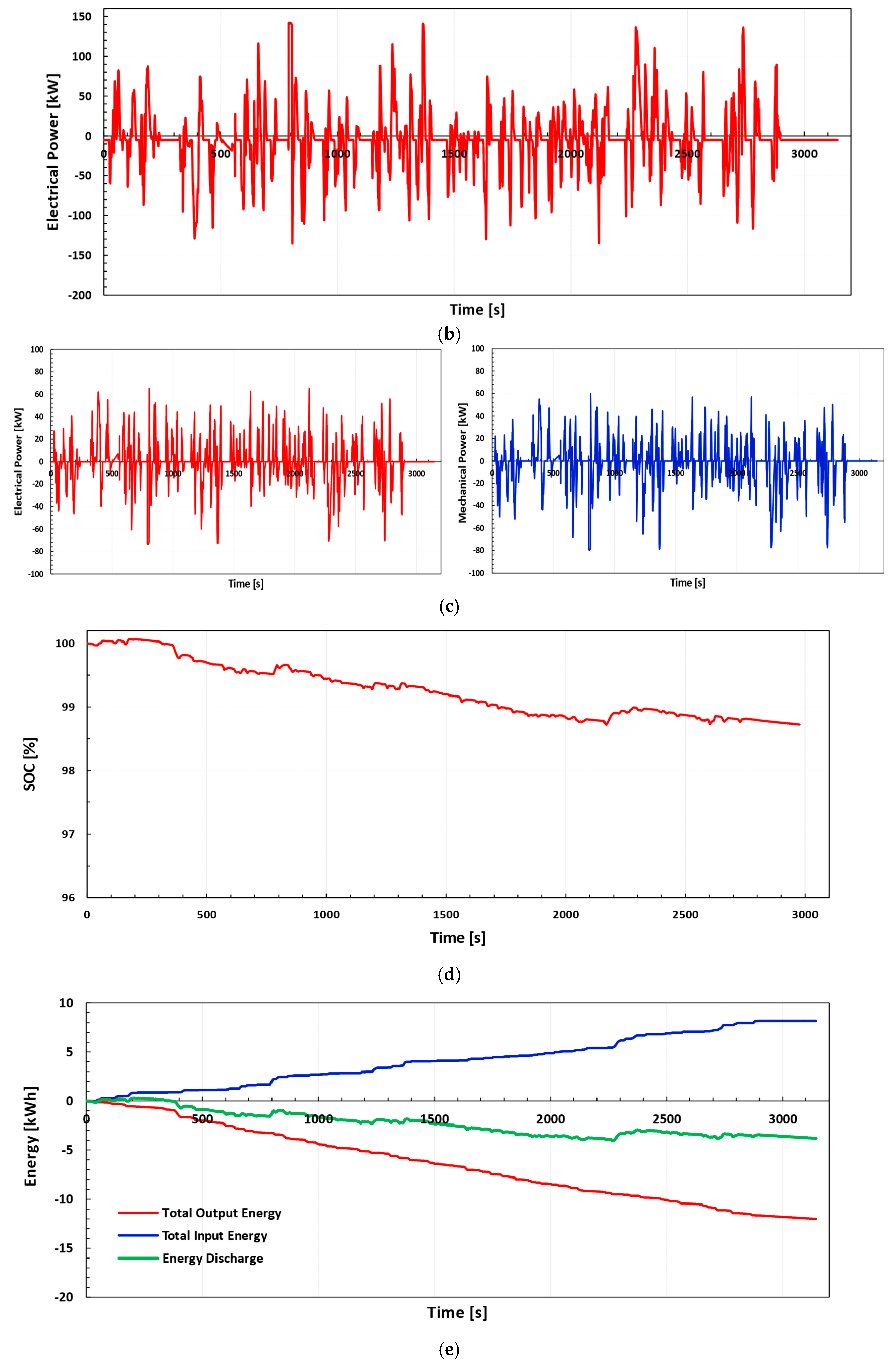
The electric machine (blocks 12 and 13) may function as an electric motor or generator that has characteristic curves for each modality. The block has two components included: a DC–AC inverter and the electric motor. To calculate losses of power and torque, a model is used with an efficiency characteristic map. The motor electric power is calculated as:

$$P_{EM{,}_{el}}=P_{E{M}_{mec}}+P_{E{M}_{loss}}$$

(20)

which is an alternative expression to Equation (8) that uses AVL Cruise and where $P_{E{M}_{loss}}$ represents lost power due to losses in iron, copper and those caused by friction. Considering the signs convection, if $P_{EM{,}_{el}}$ > 0, the motor operates in motor mode to propel the vehicle, whereas if $P_{EM{,}_{el}}$ < 0 the motor operates in generator mode, recovering part of the kinetic energy produced by the decelerations. The mechanical power can be obtained using Equation (10) as:

$$P_{E{M}_{mec}}=M_{E{M}_{out}}{\omega }_{EM}$$

(21)

The mechanical power depends strictly on angular velocity $({\omega }_{EM}),$ motor torque $\left(M_{E{M}_{out}}\right)$, and the efficiency depending on the motor’s characteristic map, which is a function of these three parameters. The efficiency map of the electric machine is shown in Figure 10.

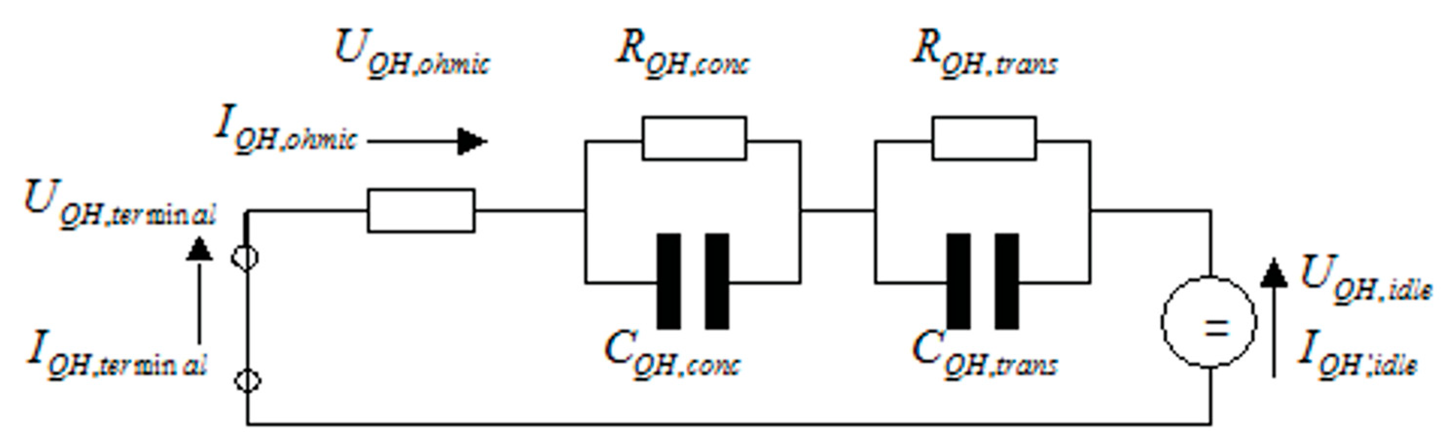
The battery (block 17) was treated as a model that consists of a source of power and resistance. The resistance model allowed us to consider the complex internal processes of the battery (Figure 11). Two optional resistor–capacitor (RC) elements were added to describe the concentration overvoltage and the transition over-voltage [54]. The dependence on temperature in resistance can be activated as an option. Individual cells may be modelled as well as combinations thereof, meaning any module may be constructed. A thermal model describes the batteries thermal behaviour. Here, heat caused by losses and cooling caused by convection were considered. This model allows the use of “the temperature and SOC-dependent” option. As such, the resistance and capacitances are dependent on temperature $\left(T_{QH}\right)$ and the charge status $\left(SO{C}_{QH}\right)$. The equation concerning output voltage on a battery cell ($U_{QH{,}_{terminal}}$) is:

$$\begin{gathered} U_{QH{,}_{terminal}}=U_{QH{,}_{idle}}\left(T_{QH,}SO{C}_{QH}\right)-I_{QH{,}_{ohmic}}{R}_{QH}\left(T_{QH,}SO{C}_{QH}\right)- \\ \frac{Q_{QH{,}_{conc}}}{C_{QH{,}_{conc}}}\left(T_{QH,}SO{C}_{QH}\right)-\frac{Q_{QH{,}_{trans}}}{C_{QH{,}_{trans}}}\left(T_{QH,}SO{C}_{QH}\right) \end{gathered}$$

(22)

where $U_{QH{,}_{idle}}$ is the idle voltage of a cell, $T_{QH}$ is the actual temperature of the battery, $SO{C}_{QH}$ is the state of charge of a cell, $I_{QH{,}_{ohmic}}$ is the actual current through the cell, $R_{QH}$ is the internal resistance, $Q_{QH{,}_{conc}}$ is the charge of the capacitance for concentration overvoltage, $C_{QH{,}_{conc}}$ is the capacitance concentration overvoltage, $Q_{QH{,}_{trans}}$ is the charge of the capacitance for transfer overvoltage, and $C_{QH{,}_{trans}}$ is the capacitance transfer overvoltage.

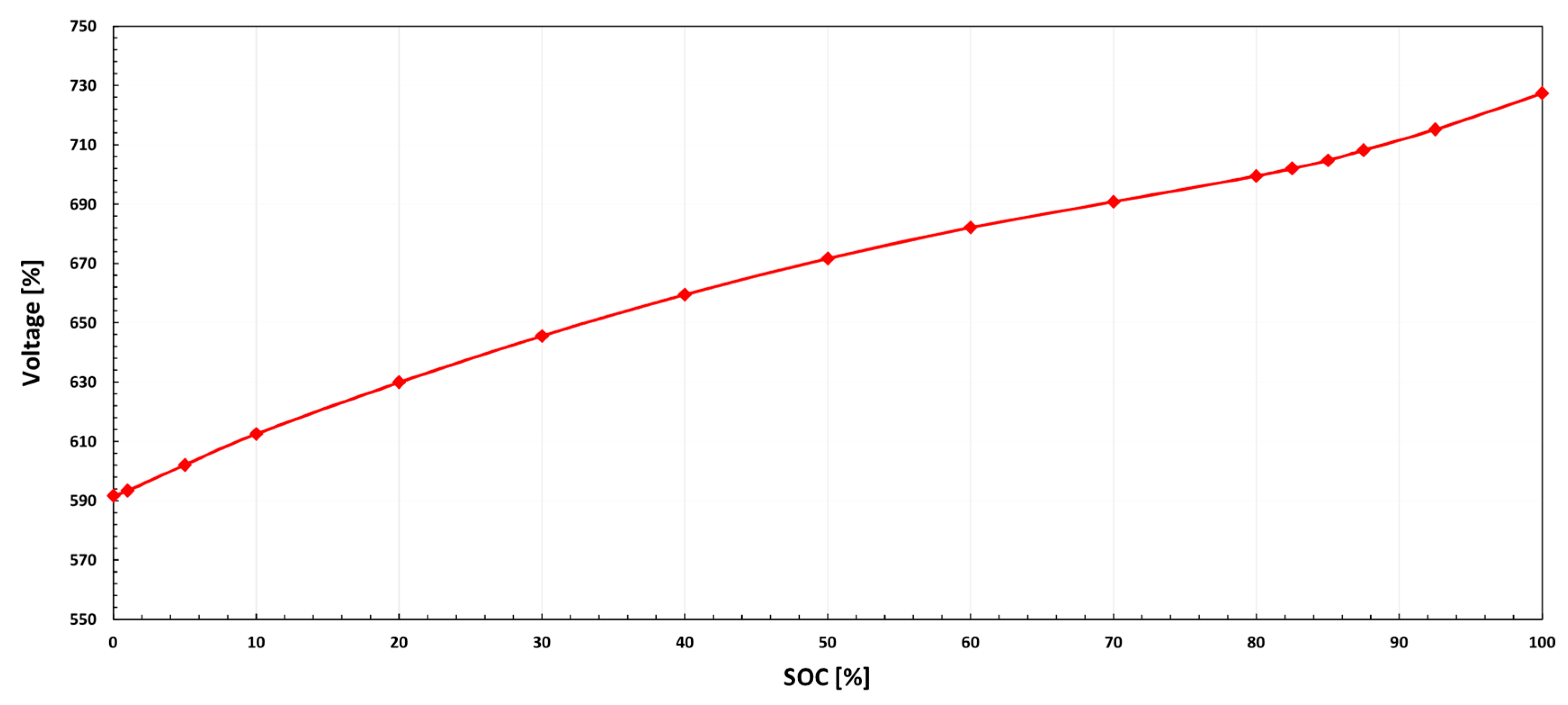
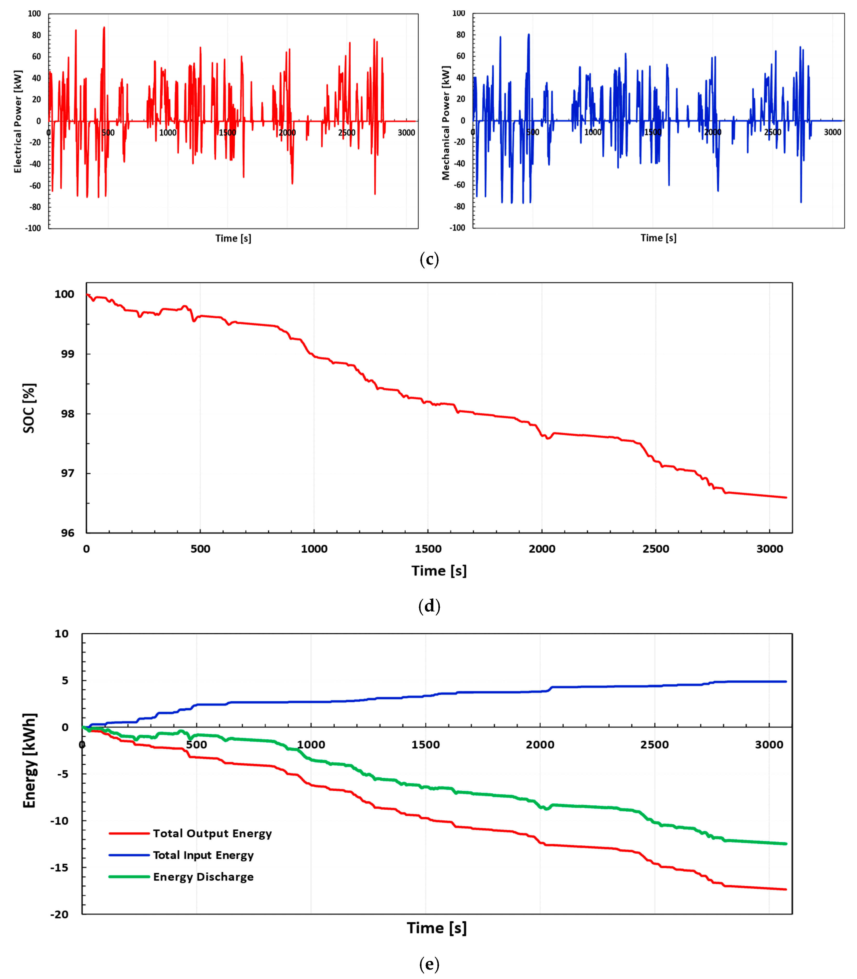
The SOC curve (Figure 12) of the battery pack was loaded into the simulation tool, which is dependent on the chosen battery technology.

The auxiliary systems are defined in the model as consumers of electricity. They are symbolised by a single block (block 16) that represents an ohmic resistance where there are losses in electric current, meaning there is power consumption. The software allows setting the resistance value as constant, or via characteristics curves. In the model concerned, we used constant resistance, considering an average working power during the complete cycle. The instant current can be calculated using the following equation:

$$I_X=\frac{U_{X{,}_{net}}}{R_{X{,}_{act}}}$$

(23)

where $I_X$ is the current, $U_{X{,}_{net}}$ is the net voltage, and $R_{X{,}_{act}}$ is the actual internal resistance.

The model shows supplementary components, such as the final drive (blocks 2 and 3), that represent the final transmission ratio of the vehicle. The vehicle’s brakes (blocks 8–11) are described using braking data and dimensions as well as a specific braking factor. The cockpit (block 14) is the component charged with connecting the driver to the vehicle; connections form using the data bus. The ASC (block 15) represents the component that controls the individual wheel friction coefficients. If a friction coefficient exceeds the maximum transferable value, the accelerator position will vary. The DC–DC converter (block 18) is a component that is used to transform, in a highly efficient manner, continuous current voltages. Its function in this model was to set the voltage for the auxiliary systems, allowing the correct flow of energy in the data bus system.

The eDrive control system (block 19) and eBrake and mBrake unit (block 20), are functions defined by the user, with its programming using C language. The eDrive function corresponds to control of the electric motor and the eBrake function acts on regenerative braking control.

The monitor (block 21) allows viewing certain calculation results while the simulation is running. Finally, block 22 provides the constants, where the values are defined and may be used by other blocks using the data bus.

2.3. Determination of CO₂ Emission for Electric Urban Buses by the Grid Power Generation

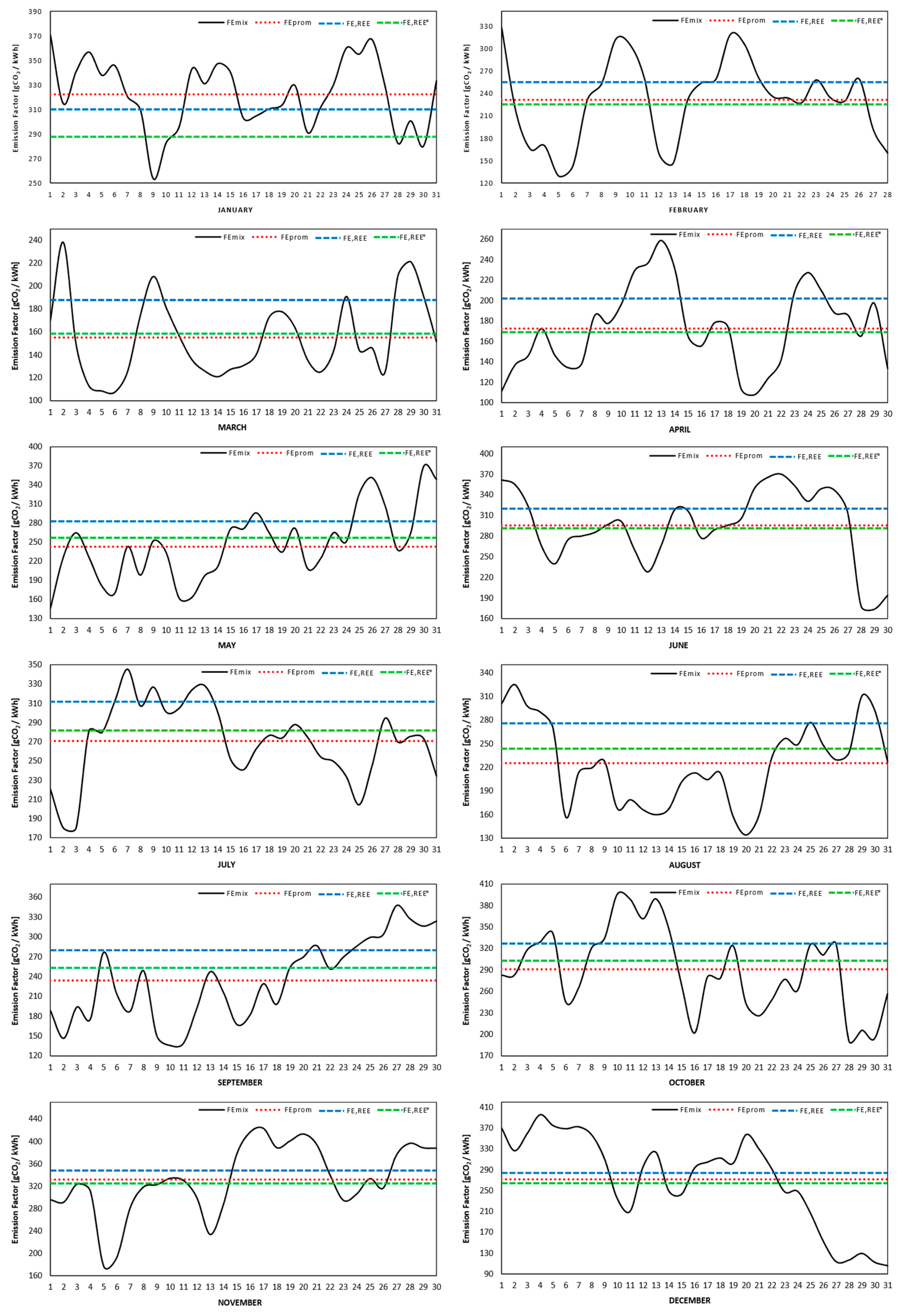
The emission component to be measured was CO₂; there was no database for the emission factors of the other power generation components [12,13]. To determine the CO₂ emissions of an electric vehicle, the electric generation should be considered. For this case, we studied the emission factors (FE) of the Spanish electricity mix. The emission factor of each power station must be associated with its contribution in terms of energy for the electric grid. The emission factors of the various power stations according to the Electric Grid of Spain (REE) [29] is shown in

Table 8. CO₂ emission factor (FE) by type of electricity generator.

Electricity Generator	FE (gCO2/kWh)
Coal	950
Wind	0
Hydroelectric	0
Biomass	0
Solar PV	0
Nuclear	0
Combined cycle (Gas)	370
Cogeneration CHP	370
Non-renewable waste	240

.

The intensity of the CO₂ emission due to charging in relation to the electricity mix was established using the following equation:

$${\mathrm{EI}}_{veh}={\mathrm{FE}}_{mix}{\mathrm{C}}_{mix}$$

(24)

where ${\mathrm{EI}}_{veh}$ is the CO₂ emission intensity (gCO₂/km), ${\mathrm{FE}}_{mix}$ is the electricity mix emission factor (gCO₂/kWh), and ${\mathrm{C}}_{mix}$ is the required electric charge from the electricity mix (kWh/km).

The electricity mix emission factor $\left({\mathrm{FE}}_{mix}\right)$ depends on the type of power stations. The efficiency of each component of the electric grid and the vehicle charging system should be considered (

Table 9. Global efficiency of the components of the system when charged [55,56].

Efficiencies (%)	${\mathit{\eta }}_{\mathit{t}\mathit{r}\mathit{a}\mathit{n}\mathit{s}}$	${\mathit{\eta }}_{\mathit{d}\mathit{i}\mathit{s}\mathit{t}}$	${\mathit{\eta }}_{\mathit{c}\mathit{h}\mathit{a}\mathit{r}\mathit{g}\mathit{e}\mathit{d}}$	${\mathit{\eta }}_{\mathit{B}\mathit{A}{\mathit{T}}_{\mathit{C}\mathit{h}}}$	${\mathit{\eta }}_{\mathit{W}\mathit{T}\mathit{T}}$
Maximum Efficiency	99	93	97	95	84.84
Minimum Efficiency	98	91	95	90	76.25
Average Efficiency	98.5	92	96	92.5	80.55

). These items make up the complete energy transport process, from the generation at the power stations up to the electric bus batteries. ${\mathrm{C}}_{mix}$ is calculated using the following equations:

$${\mathrm{C}}_{mix}=\frac{WSER}{{\eta }_{WTT}}$$

(25)

$${\eta }_{WTT}={\eta }_{trans}{\eta }_{dist}{\eta }_{charged}{\eta }_{BA{T}_{Ch}}$$

(26)

where $WSER$ is the wall-socket electricity requirement, ${\eta }_{WTT}$ is the well-to-tank efficiency, ${\eta }_{trans}$ is the efficiency of transmission, ${\eta }_{dist}$ is the efficiency of distribution, ${\eta }_{charged}$ is the efficiency of the charger (connector-battery), and ${\eta }_{BA{T}_{Ch}}$ is the battery efficiency when charged.

Definition of Scenarios

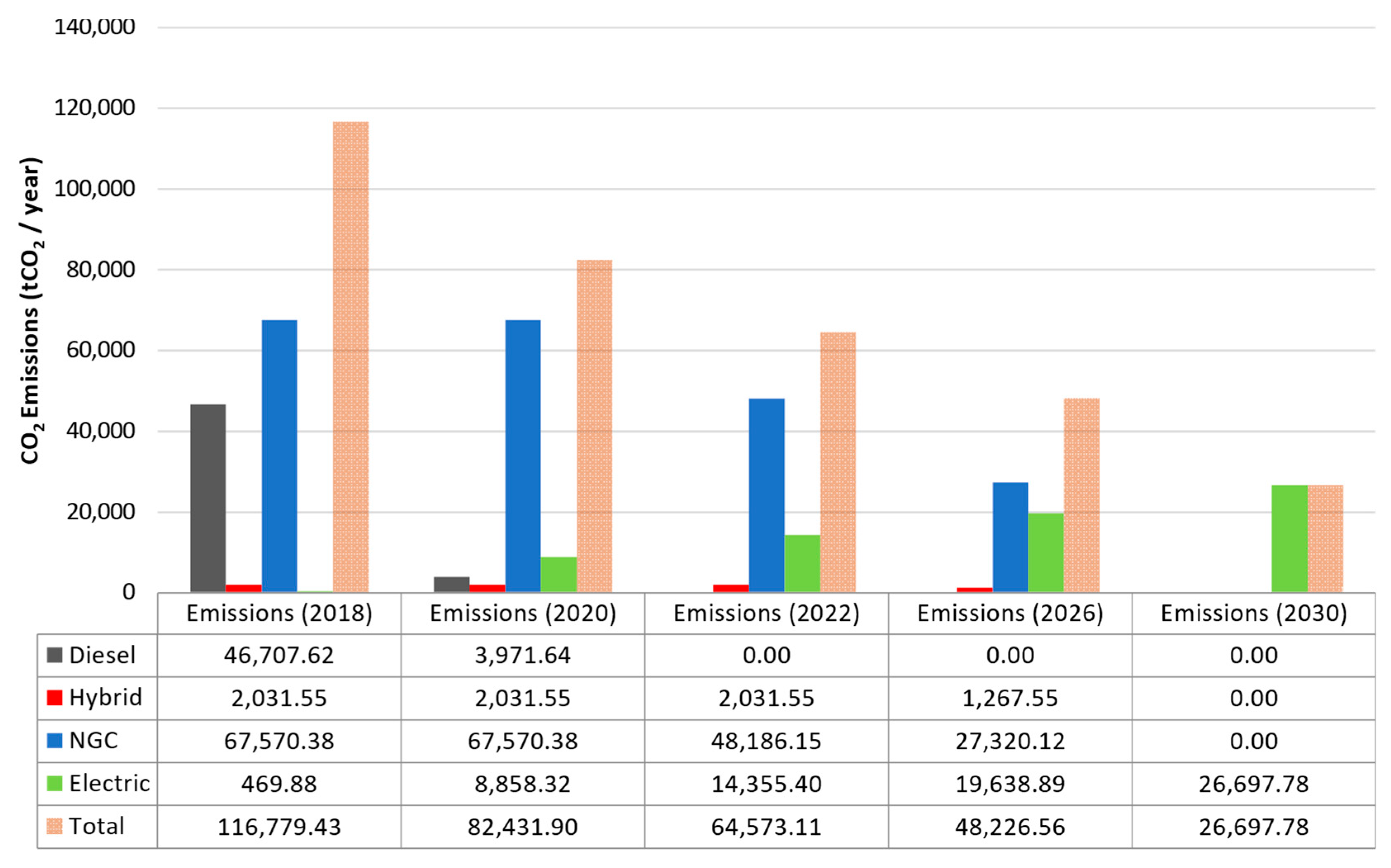
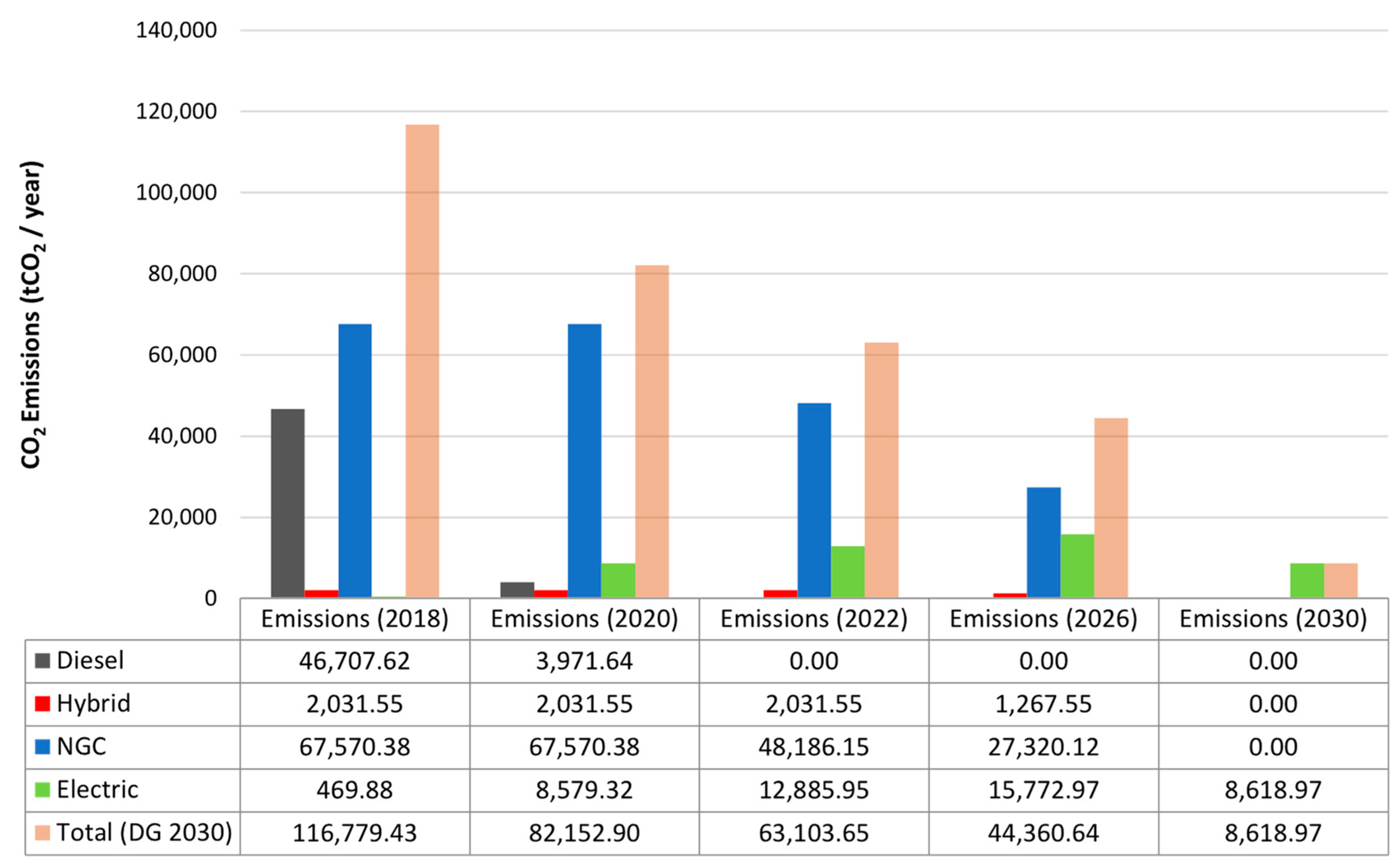
A gradual replacement of the fleet was considered, then we estimated the CO₂ emissions for the base year (2018) and those in 2020 (phase 1), 2022 (phase 2), 2026 (phase 3), and 2030 (phase 4). For the analysis, various data were obtained from scientific literature, OEMs, and EMT reports. For energy consumption and the intensity of the CO₂ emissions, the fleet of buses were taken as a start point in previous studies [57,58,59], where the estimates were calculated based on an analysis of the well-to-tank (WTT) and tank-to-wheel (TTW). The number of daily routes per vehicle was 20, with an occupation rate of 60% [60], energy consumption of each technology related to the fleet was considered constant in time, and the vehicles were grouped in four categories based on the EMT (compressed natural gas (CNG), diesel, hybrid, electric) [60]. Finally, the Spanish electricity mix data from 2017 were used, which were updated by the REE [29].

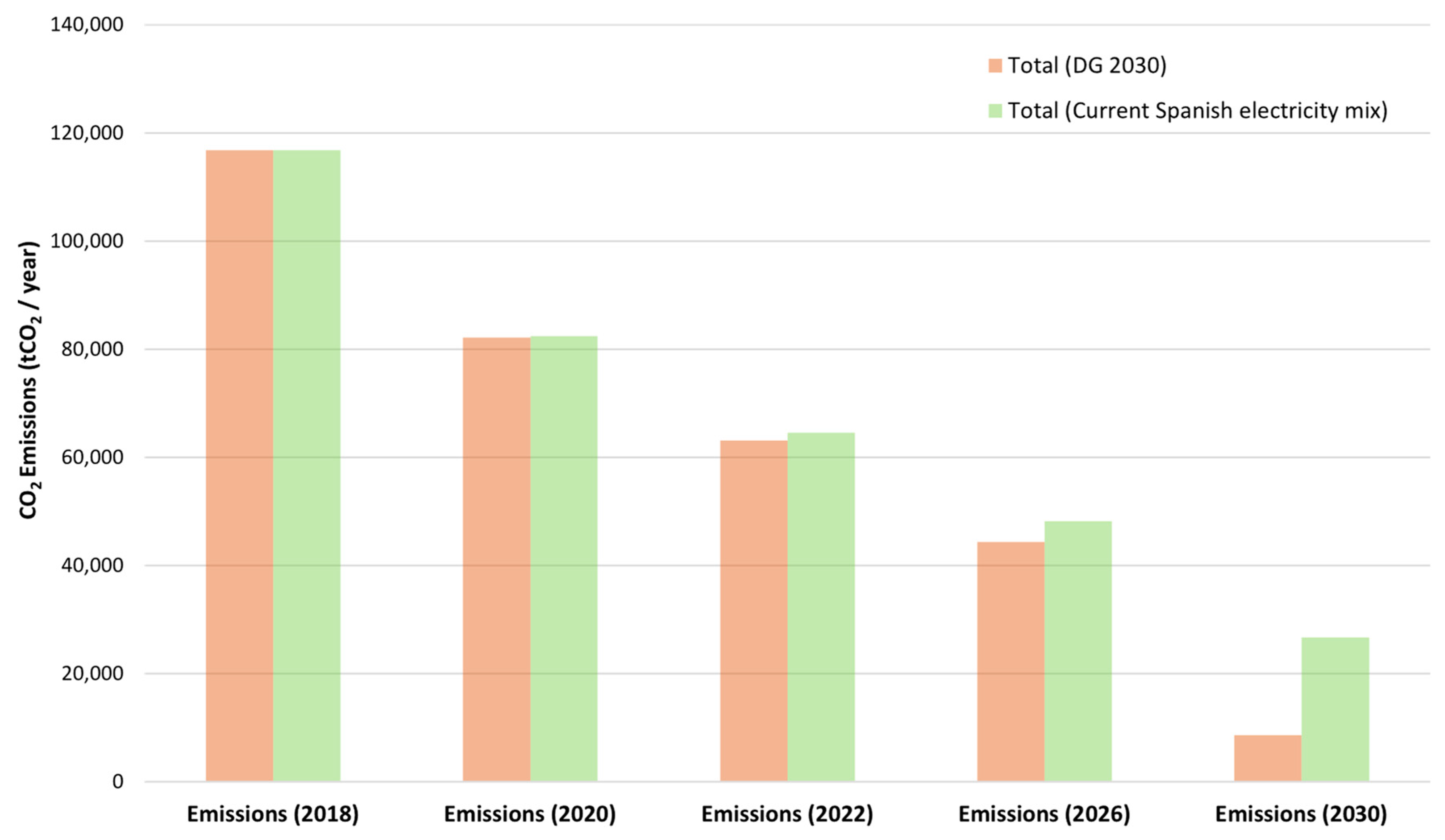
However, a change in the electricity mix is expected, which will allow the decarbonization of the electricity sector until 2030, which includes the sustainable contribution of renewable energy sources. According to expert reports, in 2030 under the DG2030 scenario, the contribution of electricity generation from renewable energies will be 62%, while that of non-renewable energies will be only 38%. This argument is analysed in results section, considering the changes that will occur in the electric mix under the 2030 distributed generation scenario, proposed by the Ten-Year Network Development Plan 2018 [61]. This is a baseline scenario upon which most of the electrical simulation exercises were based.

Table 10. Electric power sources in Spain on the Iberian Peninsula until 2030 [61,62,63,64].

Technology of Generator	Power (MW) (2017)	Power (MW) (2020)	Power (MW) (2022)	Power (MW) (2026)	Power (MW) (2030)
Renewable Energies
Wind	22,922	27,650	29,500	31,000	31,000
Hydroelectric	17,030	17,030	17,030	17,030	17,030
Solar PV	4439	5790	15,000	30,687	47,157
Solar Thermal	2304	2304	2304	3269	2300
Other renewable ()	852	1131	1131	1131	2550
Renewable waste	123	123	123	123	123
Total Renewable	47,670	54,028	65,088	83,240	100,160
Non-Renewable Energies
Combined cycle (Gas)	24,948	24,933	24,933	24,933	24,560
Coal	9536	9536	9536	9536	847
Nuclear	7117	7117	7117	7117	7117
Cogeneration CHP*	5818	6668	6668	6668	7700
Pumping	3329	3329	3329	3329	6020
Non-renewable waste	459	677	677	677	677
Total Non-renewable	51,207	52,260	52,260	52,260	46,921
Batteries					2358
Total	98,877	106,288	117,348	135,500	149,439

shows the installed power sources in the electric mix until the year 2030, whereas

Table 11. Electric generation by the power sources in Spain on the Iberian Peninsula until 2030 [61,62,63,64].

Technology of Generator	Electricity Generation (2017) (GWh)	Electricity Generation (2020) (GWh)	Electricity Generation (2022) (GWh)	Electricity Generation (2026) (GWh)	Electricity Generation (2030) (GWh)
Renewable Energies
Wind	47,498	57,295	61,129	64,237	64,923
Hydroelectric	18,361	18,361	18,361	18,361	32,257
Solar PV	7988	10,419	26,993	55,221	88,027
Solar Thermal	5348	5348	5348	7588	4589
Other renewable	3603	4783	4783	4783	13,409
Renewable waste	728	728	728	728	-
Total Renewable	83,526	96,934	117,341	150,918	203,205
Non-Renewable Energies
Combined cycle (Gas)	33,855	33,835	33,835	33,835	34,702
Coal	42,593	42,593	42,593	42,593	0
Nuclear	55,609	55,609	55,609	55,609	50,868
Cogeneration CHP	28,134	32,244	32,244	32,244	38,675
Pumping	2249	2249	2249	2249	-
Non-renewable waste	2459	3627	3627	3627	-
Total Non-renewable	164,899	170,157	170,157	170,157	124,245
Batteries					-
Total (GWh)	248,425	267,091	287,498	321,075	327,450
Total ktCO2	63,989	65,783	65,783	65,783	27,149
Emission Factor (grCO2/kWh)	257	246	228	204	82

forecasts the generation of electric power until the year 2030 foreseen under the DG2030 scenario.

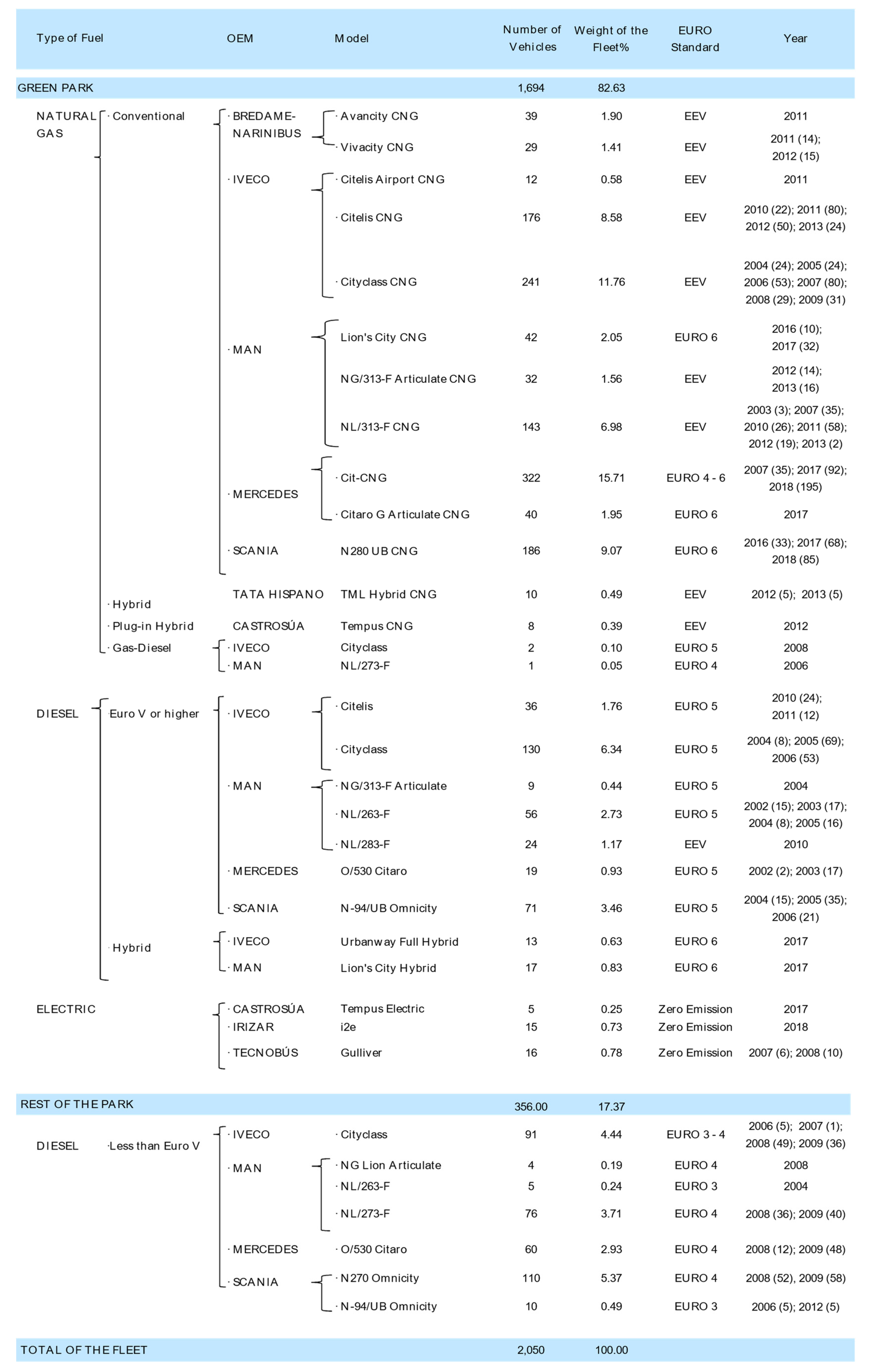
The fleet includes vehicles with various technologies, which the EMT calls the Green Park Fleet: CNG buses, diesel buses with Euro V and VI standards, pure electric buses, as well as CNG hybrid buses, while the rest of the fleet are classified as diesel buses that comply with the EURO III and IV standard. Figure 13 shows the makeup by technology of the EMT’s current fleet.

Phased replacement means there must be a gradual transition in technology change. Figure 12 shows that there is a large section of new buses as well as buses that are almost 15 years old. The phases are detailed as:

Phase 1: Corresponding to the year 2020. In this phase, all diesel buses with a standard below EURO V are replaced, as well as diesel buses registered before 2010 and CNG-diesel vehicles. In this first phase, 644 buses are replaced, corresponding to 31.42% of the total fleet.

Phase 2: Corresponding to the year 2022. In this phase, the remaining buses only powered by diesel are replaced, as are electric buses from 2007 and 2008 (fleet renewal) and CNG buses from on or before 2010. Here, we replace 438 units corresponding to 21.36% of the total fleet.

Phase 3: Corresponding to the year 2026. CNG buses from 2016 or before and CNG hybrid vehicles are replaced. In this phase, 406 buses are replaced corresponding to 19.80% of the total fleet.

Phase 4: Corresponding to the year 2030. In this final phase, all buses from 2017 and 2018 are replaced, which corresponds to 562 units, which is 27.41% of the total fleet. The electric buses replaced during these years correspond to fleet renewal, which means that by 2030, the fleet will be 100% electric.

3. Results and Discussion

3.1. Simulation Results

Figure 14a and Figure 15a show the simulation of the electric consumption of the urban bus throughout the C1 line route. The electric energy exclusively from the battery during the journey of route 1 was 12.48 kWh, whereas for route 2, it was 3.79 kWh. In Figure 14b and Figure 15b, the instant power provided by the battery pack during the journey with the maximum peak power was up to 136 kW for traction and 180 kW for regenerative braking in route 1, whereas for route 2, it was 142 kW for traction and 135 kW for regeneration.

In Figure 14c and Figure 15c (for routes 1 and 2, respectively), the electric and mechanical power in the electric machine are depicted. As expected, there were power losses $\left(P_{E{M}_{loss}}\right)$ caused by friction and iron and copper losses. Power losses occurred due to efficiency of the DC–AC inverter, which, in this model, is included in the electric motor, shown in blocks 12 and 13 of Figure 9).

The SOC curves during routes 1 and 2 can be seen in Figure 14d and Figure 15d, respectively. For route 1, the SOC was reduced by 3.83%, whereas in route 2, the SOC was reduced by 1.28%. The explanation for the higher energy consumption on route 1 is connected to the journey orography, the route starts at 628 m a.s.l. (metres above sea level) and finishes at 725 m a.s.l. (an increase of 97 m). The elevation difference for route 2 is a decrease of 97 m, starting at 725 m a.s.l. and finishing at 628 m a.s.l. This can be observed in Figure 3 and Figure 4.

Finally, in Figure 14e and Figure 15e, the total energy consumption during both routes is shown. For route 1, a total of 17.35 kWh was consumed, 12.48 kWh was provided by the battery (energy discharge), and 4.87 kWh through the regenerative braking (total input energy). For route 2, the total energy consumption of the system was 11.98 kWh, of which 3.79 kWh was from the battery itself, and 8.19 kWh from regenerative braking. The total energy used by the battery pack during a cycle was 16.27 kWh.

Table 12. Relevant results obtained during the route simulation.

Specification	Route 1	Route 2	Route Line C1
Total Output Energy (kWh)	17.35	11.98	29.33
Total Input Energy (kWh)	4.87	8.19	13.06
Electrical Consumption (kWh)	12.48	3.79	16.27
Electrical Consumption* (kWh)	124.80	37.90	162.70
Maximum Electrical Power in Traction (Batteries) (kW)	136.32	142.03	142.03
Maximum Electrical Power in Regeneration (Batteries) (kW)	180.43	134.43	180.43
Maximum Electrical Power in Traction (EM) (kW)	87.61	64.61	2 × 87.61
Maximum Electrical Power in Regeneration (EM) (kW)	70.76	73.62	2 × 73.62
Maximum Mechanical Power in Traction (EM) (kW)	80.57	59.52	2 × 80.57
Maximum Mechanical Power in Regeneration (EM) (kW)	76.57	79.44	2 × 79.44
Variation of State of Charge (ΔSOC) (%)	3.83	1.28	5.11
Variation of State of Charge** (ΔSOC) (%)	38.30	12.8	51.10

Electrical consumption* (WSER) at the end of the work day (18 h, 10 trips). Variation of state of charge** at the end of the work day (18 h, 10 trips).

summarizes the data obtained from the simulations.

3.2. Determination of CO₂ Emissions from Power Generation

The most relevant result from this analysis is the energy consumed by the electric urban bus, once the working day has been completed (Electrical Consumption*). This value is known as the wall-socket electricity requirement (WSER), which is the energy discharged by the battery during the working day. In order for the bus battery pack to return to the fully charged state, the energy consumed must be recharged (162.7 kWh). To estimate the energy when connecting the bus to the electric grid, additional losses that exist due to the efficiency of each of the electric grid systems components must be considered, such as transmission $\left({\eta }_{trans}\right),$ ad distribution (${\eta }_{dist}$), the recharging efficiency of the battery $\left({\eta }_{charged}\right),$ and the battery charging efficiency (${\eta }_{BA{T}_{Ch}}$), applying Equation (25) and considering the efficiencies in Table 9. We calculated that the energy provided by the electric grid for a full charge of the bus after a working day is 213.3 kWh in the worst case scenario, and 191.8 kWh in the best case scenario. In this study, an average efficiency was considered, meaning that the energy provided by the grid is approximately 200 kWh.

The fast charge systems for this type of application has a minimum power of 50 kW [46]. For this case, we used a charging power of 60 kW [65], meaning that complete charge occurred in 3 h 20 min. As the grid connection window is short, we considered connecting as of 12:30 a.m., which is when the bus has finished its working day, and the logistics waiting time has elapsed. As shown in Figure 16, positive factors are associated with this connection timetable, such as a larger contribution of renewable energies, especially wind power, corresponding to the valley section of the grid energy demand curve, along with a lower CO₂ rate compared with the daily average.

Figure 17 shows the analysis of the Spanish electricity mix emission factor (FE_mix) based on the demand curves every day during 2017. The emission factor during a connection between 12:30 and 3:50 a.m. (FE_prom) and the average on the Iberian Peninsula in Spain (FE,_REE*) in all cases (except January) are lower than the average Spanish electricity mix emission factor FE,_REE. This corresponds to a reduction of more than 10% in the annual emissions compared to FE_prom; however, with respect to the FE,REE*, the reduction is only 1.2%, as shown in

Table 13. Details of the emission factor in the Spanish electricity mix.

Emission Factor (FE) (g CO2/kWh)	Jan	Feb	Mar	Apr	May	Jun	Jul	Aug	Sep	Oct	Nov	Dec	Avg.
FE,REE	310	255	188	202	283	320	313	276	280	327	348	284	284
FE,REE*	287	229	157	169	254	294	286	245	250	301	327	260	257
FEprom	322	231	155	173	243	296	271	225	234	291	332	272	254
ΔFE (%)	3.9	−9.4	−17.6	−14.4	−14.1	−7.5	−13.4	−18.5	−16.4	−11.0	-4.6	−4.2	−10.6
ΔFE (%)*	12.2	0.9	−1.3	2.4	−4.3	0.7	−5.2	−8.2	−6.4	−3.3	1.5	4.6	−1.2

ΔFE (%) Variation FE,_REE versus FE_prom. ΔFE (%)* Variation FE,_REE versus FE,_REE*.

.

Table 14. Detailed results from the urban electric bus and its connection in the Spanish electricity mix.

Battery Electric Vehicle	Route Length (km)	WSER (kWh)	Electricity Mix (kWh)	Energy Consumption (kWh/km)	Cmix (kWh/km)
Urban Bus Model	175.2	162.7	200	0.93	1.15

shows a summary of the main results obtained for the urban electric bus, such as the route length, the WSER, the energy charge from the electricity mix, energy consumption and the electric charge requirement from the electricity mix (C_mix), while

Table 15. Urban bus CO₂ emission intensity to the scenario DG2030.

CO2 Emission Intensity	2018	2020	2022	2026	2030
EIveh (gCO2/km)	292.1	282.9	262.2	234.6	94.3

shows the CO₂ emission intensity from the urban bus for the years 2018, 2020, 2022, 2026, and 2030, which is the factor of emission from well-to-tank (WTT) for the electric bus that is used to determine the emissions saved compared to vehicles in the current fleet. It should be noted that the change in the Spanish electricity mix must be considered (Table 10 and Table 11), which is what is expected to be agreed on in the horizon 2030 under scenario DG2030.

To estimate the CO₂ emissions in the various fleet replacement phases, we considered previous studies [57,58,59] that analysed the life-cycles of various types of bus in the EMT fleet. For the TTW section, we used values obtained from the trials on the 15.5 km EMT route. Information was obtained in real-traffic situations based on tests with on-board equipment and subsequent modelling [34].

The results in

Table 16. Comparison of the CO₂ emissions from different buses in the fleet.

Urban Bus Technology	Weight of the Fleet (%)	Energy Consumption (kWh/100 km)	$\mathbf{E}{\mathbf{I}}_{\mathit{v}\mathit{e}\mathit{h}}-\mathbf{WTT}$ (gCO2/km)	$\mathbf{E}{\mathbf{I}}_{\mathit{v}\mathit{e}\mathit{h}}-\mathbf{TTW}$ (gCO2/km)	$\mathbf{E}{\mathbf{I}}_{\mathit{v}\mathit{e}\mathit{h}}-\mathbf{WTW}$ (gCO2/km)
Diesel *	34.34	571.19	162.14	1326.00	1488.14
Hybrid **	2.34	470.22	153.88	796,00	949.88
CNG ***	61.56	727.57	186.92	1014.00	1200.92
Electric ****	1.76	93.00	292.10	0.00	292.10

* includes all diesel buses, ** includes all hybrid buses, *** includes all CNG buses, and **** corresponds to the value simulated in AVL Cruise.

show that the energy consumption in electric buses is less than the other technologies, being six times less than diesel buses, close to eight times less than CNG buses, and five times less than hybrid buses. This is due to the high energy conversion efficiency of the electric vehicles. The emission intensity related to CO₂ emitted during the well-to-wheel (WTW) analysis shows that an electric bus is five times less polluting than a diesel bus, four times less than a CNG bus, and three times less than hybrids. In the coming years the CO₂ emission intensity will even be lower than currently, which is even more favourable for the electric vehicle.

Figure 18 shows the reduction in CO₂ emissions produced by the total implementation of a fleet of electric buses over a 10-year period with the current Spanish electricity mix (constant until 2030). The 2018 fleet was taken as a reference, having estimated emissions of 116.8 ktCO₂ for that year. During phase 1, forecast for 2020, the replacement of 31.42% of the fleet exclusively involves diesel buses. We estimated that emissions will be reduced to 82.4 ktCO₂, which is 29.41% less than 2018. In phase 2, forecast for 2022, the replacement of 21.37% of the fleet (2.93% corresponding to the remaining diesel buses, 17.66% of CNG buses, and 0.78% of the renewal of electric buses from 2007 and 2008), we estimated a reduction of 44.71% in relation to 2018, which is 64.6 ktCO₂. During phase 3, the forecast for 2026, 19.79% of the fleet is replaced (18.91% of CNG and 0.88% of CNG hybrid buses). We estimated that emissions will be reduced to 48.2 ktCO₂, which is 58.70% less than in 2018. Finally, in 2030, where the whole fleet is 100% electric, replacing the remaining 27.41% of the fleet (24.97% CNG buses, 1.46% hybrid buses, and 0.98% renewal of electric buses), emissions will be reduced to 26.7 ktCO₂, which is 77.14% less than the emissions for 2018. Figure 19 assumes the same previous conditions but with Spanish electricity mix of the horizon 2030 under the DG2030 scenario, with an emission factor of 82 gCO₂/kWh, emissions can be reduced by up to 92.6% compared to 2018. Finally, Figure 20 compares the CO₂ emissions between the two scenarios.

4. Conclusions

From the simulations we completed for an electric bus conceptual model using the AVL Cruise software using a speed and height profile for the most representative bus line route in Madrid and gradually replacing the conventional fleet for electric buses over a period of 10 years, we conclude the following:

An electric bus is more efficient as it has fewer losses in the powertrain. The results have shown that the energy consumption of electric urban buses is representatively less than the remaining technologies, six times less than conventional diesel buses, close to eight times less than CNG buses and five times less than hybrid buses.

Electric buses are less contaminating than the remaining technologies as the CO₂ emission intensity is lower, using a Well-To-Tank (WTT ) and Tank-To-Wheel (TTW) analysis it shows that an electric bus with the current Spanish electricity mix is five times less contaminant than a diesel bus, four times less than a CNG bus and three times less than a hybrid bus, as well as not emitting pollutant gases such as: NOx, CO, HC, PM₁₀, and PM_2.5, which are harmful for health.

With a Spanish electricity mix towards the horizon 2030 and under the DG2030 scenario, an electric urban bus can become representatively less contaminating than other technologies: 15 times less contaminating than a diesel bus, 13 times less than a CNG bus, and 10 times less than a hybrid bus.

• The previous studies completed by this research group have proven that by replacing the current fleet with CNG buses, despite reducing NO_x by 31.5% and completely eliminating PM, the CO₂ emissions increase by 5.1%, the HC by 307%, and CO₂ by 94.3%. This means that the most viable option, in our opinion, is the inclusion of electric urban buses if a city wishes be to radically eliminate GHG and pollution.
• Although there are still controversies about electric vehicles due to the issue of environmental impact in their manufacturing and the recycling of batteries, there are studies that show that only 13% of the CO₂ emission intensity depends on the batteries. Another factor equally important is the electricity mix that is intended to charge the vehicle. The connection of the electric vehicle to an electricity mix, such as the Spanish mix, is sustainable since 33.7% of the electric power is generated from renewable energies, which results in a lower emission factor than the average of the European Union. All these positive factors allow us to think that, in a life cycle analysis, electric vehicles are much less polluting than diesel or gasoline vehicles.

References

1. International Energy Agency (IEA). Key World Energy Statistics; IEA: Paris, France, 2017; pp. 1–97. [Google Scholar] [CrossRef]
2. International Energy Agency (IEA). CO2 emissions from fuel combustion. Oecd/Iea 2016, 1–155. [Google Scholar] [CrossRef]
3. Nederhoff, E. Transport Energy and CO2: Moving towards Sustainability; OECD iLibrary: Paris, France, 2009; ISBN 9789264073166. [Google Scholar]
4. The European Parliament and the Council of the European Union. Directive 2009/28/EC of the European Parliament and of the Council of 23 April 2009; European Union: Brussels, Belgium, 2009. [Google Scholar]
5. International Energy Agency (IEA). Energy Policy Review: Spain 2015; Energy Policies of IEA Countries; OECD Publishing: Paris, France, 2015. [Google Scholar]
6. Ministerio de Agricultura y Pesca; Alimentación y Medio Ambiente. Inventario Nacional de Emisiones de Gases de Efecto Invernadero 1990–2016; Ministerio de Agricultura y Pesca: Madrid, Spain, 2018.
7. International Association of Public Transport. Public Transport Moving Europe Forward. Available online: https://www.uitp.org/sites/default/files/cck-focus-papers-files/PUBLIC TRANSPORT - MOVING EUROPE FORWARD.pdf (accessed on 17 October 2018).
8. Tribioli, L. Energy-Based Design of Powertrain for a Re-Engineered Post-Transmission Hybrid Electric Vehicle. Energies 2017, 10, 918. [Google Scholar] [CrossRef]
9. Kivekäs, K.; Lajunen, A.; Vepsäläinen, J.; Tammi, K. City bus powertrain comparison: Driving cycle variation and passenger load sensitivity analysis. Energies 2018, 11, 1755. [Google Scholar] [CrossRef]
10. Proterra. CATALYST®: 40 FOOT BUS SPECIFICATIONS FC Series XR Series E2 Series. Available online: https://www.proterra.com/wp-content/uploads/2016/08/Proterra-Catalyst-Vehicle-Specs.pdf (accessed on 20 July 2018).
11. Nordic Energy Research. Copenhagen trial with 12 m B.Y.D K9 electric buses. Available online: http://www.nordicenergy.org/wp-content/uploads/2018/02/3.-Test-of-large-charged-electric-buses-in-Copenhagen-Victor-Hug.pdf (accessed on 26 July 2018).
12. Varga, B.O. Electric vehicles, primary energy sources and CO2 emissions: Romanian case study. Energy 2013, 49, 61–70. [Google Scholar] [CrossRef]
13. Teixeira, A.C.R.; Sodré, J.R. Impacts of replacement of engine powered vehicles by electric vehicles on energy consumption and CO2 emissions. Transp. Res. Part D Transp. Environ. 2018, 59, 375–384. [Google Scholar] [CrossRef]
14. Auto, B. K7 Electric Transit Bus. Available online: http://en.byd.com/usa/wp-content/uploads/2018/04/k7m.pdf (accessed on 20 July 2018).
15. BYD Auto. K9s Electric Transit Bus. Available online: http://en.byd.com/usa/wp-content/uploads/2018/04/k9s.pdf (accessed on 20 July 2018).
16. BYD Auto. K9 Electric Transit Bus. Available online: http://en.byd.com/usa/wp-content/uploads/2018/04/k9mc.pdf (accessed on 20 July 2018).
17. BYD Auto. K11 Electric Transit Bus. Available online: http://en.byd.com/usa/wp-content/uploads/2017/06/k11.pdf (accessed on 20 July 2018).
18. BYD Auto. C6 Electric Motor Coach. Available online: http://en.byd.com/usa/wp-content/uploads/2018/04/c6.pdf (accessed on 20 July 2018).
19. BYD Auto. C9 Electric Motor Coach. Available online: http://en.byd.com/usa/wp-content/uploads/2018/04/c9.pdf (accessed on 20 July 2018).
20. BYD Auto. C10 Electric Motor Coach. Available online: http://en.byd.com/usa/wp-content/uploads/2017/06/c10.pdf (accessed on 20 July 2018).
21. IRIZAR S. Coop. i2e: Autobús urbano de 12m con tracción y clima%zación 100% eléctrica. Available online: http://www.irizar.com/wp-content/uploads/2016/02/Caso-Práctico-IHOBE.pdf (accessed on 18 July 2018).
22. DesignLine Corporation. DesignLine Eco-Smart I. Available online: https://cptdb.ca/wiki/index.php?title=DesignLine_Eco-Smart_I (accessed on 16 July 2018).
23. EBUSCO®. EBUSCO® ELECTRIC CITYBUS 2.1. Available online: https://ebusco.eu/electric-buses/#top (accessed on 10 July 2018).
24. Bloch-Rubin, T.; Gallo, J.-B.; Tomic, J. Peak Demand Charges and Electric Transit Buses; U.S. Energy Information Agency: Washington, DC, USA, 2014; Volume 5605.
25. New Flyer Industries. Xcelsior CHARGETM. Available online: https://www.newflyer.com/site-content/uploads/2018/03/Xcelsior-CHARGE-compressed.pdf (accessed on 14 July 2018).
26. ZEPS Technology. Available online: http://zepsdrive.com/technology/ (accessed on 15 July 2018).
27. COP 21 Paris France Sustainable Innovation Forum 2015 working with UNEP. Available online: http://www.cop21paris.org/ (accessed on 14 November 2018).
28. 2020 climate; Energy Package | Climate Action. Available online: https://ec.europa.eu/clima/policies/strategies/2020_en (accessed on 14 November 2018).
29. Red Eléctrica de España. Demanda Peninsular de Energía en tiempo real. Available online: https://www.ree.es/es (accessed on 13 November 2018).
30. Red Eléctrica de España. El sistema electrico Español 2017. Available online: https://www.ree.es/es (accessed on 13 November 2018).
31. Messagie, M. Life Cycle Analysis of the Climate Impact of Electric Vehicles. Transp. Environ. 2017, 1–14. [Google Scholar]
32. EMT Madrid. Empresa Municipal de Transportes de Madrid, S.A. Principales Cifras. Available online: https://www.emtmadrid.es/Elementos-Cabecera/Enlaces-Pie-vertical/EMPRESA/Somos/Principales-cifras-(1) (accessed on 18 October 2018).
33. EMT Madrid. Empresa Municipal de Transportes de Madrid, S.A. PLAN ESTRATÉGICO 2017–2020. Available online: https://www.emtmadrid.es/Ficheros/Plan-Estrategico-2017-2020.aspx (accessed on 13 November 2018).
34. López-Martínez, J.M.; Jiménez, F.; Páez-Ayuso, F.J.; Flores-Holgado, M.N.; Arenas, A.N.; Arenas-Ramirez, B.; Aparicio-Izquierdo, F. Modelling the fuel consumption and pollutant emissions of the urban bus fleet of the city of Madrid. Transp. Res. Part D Transp. Environ. 2017, 52, 112–127. [Google Scholar] [CrossRef]
35. Jiménez, F.; Román, A.; López, J.M. Methodology for kinematic cycle characterization of vehicles with fixed routes in urban areas. Transp. Res. Part D Transp. Environ. 2013, 22, 14–22. [Google Scholar] [CrossRef]
36. Jiménez Alonso, F.; Román, A.; Lopez Martinez, J.M. Determinación De Ciclos De Conducción En Rutas Urbanas Fijas. Dyna Ing. E Ind. 2013, 88, 681–688. [Google Scholar] [CrossRef]
37. Jiménez, F.; Serradilla, F.; Román, A.; Naranjo, J.E. Bus line classification using neural networks. Transp. Res. Part D Transp. Environ. 2014, 30, 32–37. [Google Scholar] [CrossRef]
38. Jiménez, F.; Román, A. Urban bus fleet-to-route assignment for pollutant emissions minimization. Transp. Res. Part E 2016, 85, 120–131. [Google Scholar] [CrossRef]
39. Łebkowski, A. Steam and Oxyhydrogen Addition Influence on Energy Usage by Range Extender—Battery Electric Vehicles. Energies 2018, 11, 2403. [Google Scholar] [CrossRef]
40. Mallon, K.; Assadian, F.; Fu, B.; Mallon, K.R.; Assadian, F.; Fu, B. Analysis of On-Board Photovoltaics for a Battery Electric Bus and Their Impact on Battery Lifespan. Energies 2017, 10, 943. [Google Scholar] [CrossRef]
41. Ehsani, M.; Gao, Y.; Emadi, A. Modern Electric, Hybrid Electric, and Fuel Cell Vehicles: Fundamentals, Theory, and Design; CRC Press: Boca Raton, FL, USA, 2017. [Google Scholar]
42. Aparicio, F.; Vera, C.; Díaz, V. Teoría de los Vehículos Automóviles; Sección Publicaciones la ETSII-UPM; ETSII-UPM: Madrid, Spain, 1995. [Google Scholar]
43. Grijalva, E.; López Martínez, J.; Flores, M.; del Pozo, V. Design and Simulation of a Powertrain System for a Fuel Cell Extended Range Electric Golf Car. Energies 2018, 11, 1766. [Google Scholar] [CrossRef]
44. Commission of the European Communities. Implementing Directive 2005/32/EC of the European Parliament and of the Council with Regard to Ecodesign Requirements for Electric Motors (Text with EEA Relevance); Commission of the European Communities: Brussels, Belgium, 2009. [Google Scholar]
45. Siemens ELFA Components Data Sheets. Available online: https://www.industry.usa.siemens.com/drives/us/en/electric-drives/hybrid-drives/automotive/Documents/elfa-components-data-sheets.pdf (accessed on 14 November 2018).
46. International Energy Agency. Global EV Outlook 2018; International Energy Agency Publications: Paris, France, 2018. [Google Scholar]
47. Gao, D.; Jin, Z.; Zhang, J.; Li, J.; Ouyang, M. Development and performance analysis of a hybrid fuel cell/battery bus with an axle integrated electric motor drive system. Int. J. Hydrog. Energy 2016, 41, 1161–1169. [Google Scholar] [CrossRef]
48. Gao, D.; Jin, Z.; Zhang, J.; Li, J.; Ouyang, M. Comparative study of two different powertrains for a fuel cell hybrid bus. J. Power Sources 2016, 319, 9–18. [Google Scholar] [CrossRef]
49. De Miranda, P.E.V.; Carreira, E.S.; Icardi, U.A.; Nunes, G.S. ScienceDirect Brazilian hybrid electric-hydrogen fuel cell bus: Improved on-board energy management system. Int. J. Hydrog. Energy 2017, 42, 13949–13959. [Google Scholar] [CrossRef]
50. Gao, Z.; Daw, C.S.; Smith, D.E.; LaClair, T.J.; Parks, J.E.; Jones, P.T. Comparison of Parallel and Series Hybrid Power Trains for Transit Bus Applications. Transp. Res. Rec. J. Transp. Res. Board 2016, 2570, 97–106. [Google Scholar] [CrossRef]
51. Gao, Z.; Lin, Z.; LaClair, T.J.; Liu, C.; Li, J.M.; Birky, A.K.; Ward, J. Battery capacity and recharging needs for electric buses in city transit service. Energy 2017, 122, 588–600. [Google Scholar] [CrossRef]
52. Göhlich, D.; Kunith, A.; Ly, T. Technology assessment of an electric urban bus system for berlin. WIT Trans. Built Environ. 2014, 138, 137–149. [Google Scholar] [CrossRef]
53. Burke, A.; Jungers, B.; Yang, C.; Ogden, J. Battery Electric Vehicles: An Assessment of the Technology and Factors Influencing Market Readiness. Available online: http://samersanaat.com/en/wp-content/uploads/2012/07/AEP_Tech_AssessmentBEVs.pdf (accessed on 5 July 2018).
54. Nájera, J.; Moreno-Torres, P.; Lafoz, M.; de Castro, R.M.; Arribas, J.R. Approach to Hybrid Energy Storage Systems Dimensioning for Urban Electric Buses Regarding Efficiency and Battery Aging. Energies 2017, 10, 1708. [Google Scholar] [CrossRef]
55. Faria, R.; Marques, P.; Moura, P.; Freire, F.; Delgado, J.; de Almeida, A.T. Impact of the electricity mix and use profile in the life-cycle assessment of electric vehicles. Renew. Sustain. Energy Rev. 2013, 24, 271–287. [Google Scholar] [CrossRef]
56. Smith, W.J. Can EV (electric vehicles) address Ireland’s CO2emissions from transport? Energy 2010, 35, 4514–4521. [Google Scholar] [CrossRef]
57. García Sánchez, J.A.; López Martínez, J.M.; Lumbreras Martín, J.; Flores Holgado, M.N.; Aguilar Morales, H. Impact of Spanish electricity mix, over the period 2008-2030, on the Life Cycle energy consumption and GHG emissions of Electric, Hybrid Diesel-Electric, Fuel Cell Hybrid and Diesel Bus of the Madrid Transportation System. Energy Convers. Manag. 2013, 74, 332–343. [Google Scholar] [CrossRef]
58. Antonio García Sánchez, J.; María López Martínez, J.; Lumbreras Martín, J.; Nuria, M.; Holgado, F. Comparison of Life Cycle energy consumption and GHG emissions of natural gas, biodiesel and diesel buses of the Madrid transportation system. Energy 2012, 47, 174–198. [Google Scholar] [CrossRef]
59. Antonio Garcia-Sanchez, J.; Maria Lopez-Martinez, J.; Flores-Holgado, N.; Arenas-Ramirez, B. Life Cycle Analysis of Euro IV urban buses. Dyna 2012, 87, 45–57. [Google Scholar] [CrossRef]
60. EMT-Madrid-Informe-de-Gestion-2017. Available online: https://www.emtmadrid.es/Ficheros/Informes-Anuales/EMT-Madrid-Informe-de-Gestion-2017.aspx (accessed on 23 November 2018).
61. Ministerio de Industria Comercio y Turismo de España. Comisión de Expertos de Transición Energética. Análisis y propuestas para la descarbonización. Available online: https://www.mincotur.gob.es/es-es/GabinetePrensa/NotasPrensa/2018/Documents/Resumen 20180402 Veditado.pdf (accessed on 5 January 2019).
62. Centro de Investigaciones Energéticas—Medioambientales y Tecnológicas. Informe de transición del sector eléctrico horizonte 2030. Available online: http://www.ciemat.es/cargarAplicacionAgenda.do;jsessionid=DC42B2026385A53B0FAFC1F286AC8D20?identificador=2920 (accessed on 8 January 2019).
63. Pradas, I.G. Propuesta de equilibrio del sistema eléctrico español para 2030 y su impacto global. Tecnica Ind. 2017, 64–73. [Google Scholar] [CrossRef]
64. Comisión Nacional de los Mercados y la Competencia. Informe de supervisión del mercado peninsular de producción de energía eléctrica. Available online: https://www.cnmc.es/listado/sucesos_energia_mercado_electrico_informes_de_supervision_del_mercado_mayorista_spot/block/250 (accessed on 8 January 2019).
65. Norregaard, K.; Johnsen, B.; Hedegaard Gravesen, C. Battery degradation in electric buses. Available online: https://www.trafikstyrelsen.dk/~/media/Dokumenter/06%20Kollektiv%20trafik/Forsogsordningen/2013/Elbusser/Battery%20degradation%20in%20electric%20buses%20-%20final.pdf (accessed on 20 September 2018).
Figure 1. Urban lines: Circular C1 (yellow), Line 27 (blue), and Line 63 (green).
Energies 12 00525 g001
Figure 2. On-road standard testing route. Circular C1 Bus line (purple section shows route 1; white section shows route 2).
Energies 12 00525 g002
Figure 3. Actual speed and height profiles for a typical result along route 1.
Energies 12 00525 g003
Figure 4. Actual speed and height profiles for a typical result along route 2.
Energies 12 00525 g004
Figure 5. Configuration of the Electric Urban Bus.
Energies 12 00525 g005
Figure 6. Physical factors required to model and design the propulsion system.
Energies 12 00525 g006
Figure 7. Typical micro-cycle in an urban route. Line 27 EMT-Madrid.
Energies 12 00525 g007
Figure 8. Power and torque characteristics of traction motor versus motor rpm.
Energies 12 00525 g008
Figure 9. Electric urban bus model.
Energies 12 00525 g009
Figure 10. Electric machine efficiency map.
Energies 12 00525 g010
Figure 11. Substitution model of a battery cell.
Energies 12 00525 g011
Figure 12. State of charge (SOC) of the battery pack.
Energies 12 00525 g012
Figure 13. EMT (Madrid Municipal Transport Company) urban bus fleet.
Energies 12 00525 g013
Figure 14. Route 1: (a) speed profile and cumulative energy consumption, (b) instantaneous power of traction battery, (c) electrical (red) and mechanical power (blue), (d) state of charge consumption during the cycle, and (e) energy consumption during the cycle.
Energies 12 00525 g014aEnergies 12 00525 g014b
Figure 15. Route 2: (a) speed profile and cumulative energy consumption; (b) instantaneous power of traction battery; (c) electrical (red) and mechanical power (blue); (d) state of charge consumption during the cycle; (e) energy consumption during the cycle.
Energies 12 00525 g015aEnergies 12 00525 g015b
Figure 16. Typical load demand of the Spain electricity mix (July 30, 2017 [29]).
Energies 12 00525 g016
Figure 17. CO2 emissions factors of the Spanish electricity mix for the year 2017.
Energies 12 00525 g017
Figure 18. Comparison of the estimated CO2 emissions for different bus fleet phases substitution with the current Spanish electricity mix.
Energies 12 00525 g018
Figure 19. Comparison of the estimated CO2 emissions for different bus fleet phases substitution with the Spanish electricity mix DG2030.
Energies 12 00525 g019
Figure 20. Comparison of the estimated CO2 emissions between the current Spanish electricity mix and DG2030 scenario.
Energies 12 00525 g020