Article

Time-Aware Monitoring of Overhead Transmission Line Sag and Temperature with LoRa Communication

1
Faculty of Electrical Engineering and Computer Science, Lublin University of Technology, 20-618 Lublin, Poland
2
Faculty of Mathematics, Physics and Computer Science, Maria Curie-Sklodowska University, 20-031 Lublin, Poland
*
Author to whom correspondence should be addressed.
Energies 2019, 12(3), 505; https://doi.org/10.3390/en12030505
Submission received: 18 December 2018 / Revised: 18 January 2019 / Accepted: 30 January 2019 / Published: 5 February 2019
(This article belongs to the Special Issue Operation and Control of Power Distribution Systems)

Abstract

:
The techniques of Dynamic Line Rating (DLR) for Overhead Transmission Line (OTL)’s are currently dynamically developed. DLR systems typically rely on weather, temperature, inclination, and current measurements to calculate tension and sag, where sensors need to be installed directly on wires. Such systems are very reliable and ensure high accuracy in determining maximum allowable current. However, their installation may require switching off the transmission line from the operation. In order to receive precise values regarding the actual operating conditions of the whole transmission line, DLR sensors measuring wire temperature or tension should be installed at many points of OTL. The minimum number of installation points should cover at least each tension section and critical spans, thereby increasing installation costs. The alternative method that allows for the monitoring of OTL is the use of the vision system based on cameras. Installed on the OTLs’ poles, cameras can take photos which, appropriately processed, can provide data about the sag and temperature of wires, without the necessity of switching OTL from the operation for installation or further maintenance. Such a vision system facilitates also data transmission, because it does not require measurement data to be transmitted from the sensor station installed on the wire to the base station located on the pole (for instance, via radio). This article aims to present the concept of a vision system that monitors sag and temperature of Overhead Transmission Lines (OTLs)’ using Long Range (LoRa) wireless communication and data transmission. The developed system consists of a camera and a microcomputer equipped with LoRa communication module. The whole system monitors OTLs’ spans by taking photos, processing images for wire sag-temperature estimation, and sending results to the operator’s Supervisory Control And Data Acquisition (SCADA). The system communication architecture is also proposed and investigated for data transmission time when monitoring the whole OTL.

1. Introduction

The techniques of DLR for OTLs are currently dynamically developed. DLR systems typically rely on weather, temperature, inclination, and current measurements to calculate tension and sag, where sensors need to be installed directly on wires. Such systems are very reliable and ensure high accuracy in determining maximum allowable current. However, their installation may require switching off the transmission line from the operation. In order to receive precise values regarding the actual operating conditions of the whole transmission line, DLR sensors measuring wire temperature or tension should be installed at many points of OTL. The minimum number of installation points should cover at least each tension section and critical spans, thereby increasing installation costs. The alternative method that allows for the monitoring of OTL is the use of the vision system based on cameras. Installed on the OTLs’ poles, cameras can take photos which, appropriately processed, can provide data about sag and temperature of wires, without the necessity of switching OTL from the operation for installation or further maintenance. Such a vision system facilitates also data transmission, because it does not require measurement data to be transmitted from sensor station installed on the wire to the base station located on the pole (for instance, via radio).

1.1. Related Work

There exist many successfully installed and developed DLR systems [1,2,3,4,5,6,7], which can be used for improving the accuracy of power system models [8,9] and then applied for optimal generation scheduling [10], or congestion management [11,12]. In typical DLR solutions [13], measuring stations equipped with temperature [14], elongation [15], strain, or inclination sensors [16,17] are mounted directly on the transmission line wires [14,15,16]. Such sensor stations are usually powered by a rechargeable battery during a normal line operation [11]. The measuring station typically communicates with the base station, using radio or other applicable wireless communication technology [18,19]. In the case of the measurements provided with a direct fiber-optic cable [14,16], the radio communication between sensor head and base station can be neglected. The installation of measuring stations on wires is usually performed when the power line is out of service, which in some cases can be challenging to achieve. There are techniques that allow for mounting sensor stations on the energized power line. However, in the case of high voltage lines and due to human safety, such a technique is avoided.

1.2. Motivation and Contribution

To facilitate the DLR system installation and future maintenance, there are alternative contactless monitoring methods of OTLs’ operational state [20,21], such as temperature, sag, or icing [13,17,22]. One of the many possibilities of OTL contactless monitoring can be the usage of cameras mounted on the lines’ poles [1,20,23,24]. The data concerning the actual operational state can be sent to the SCADA system via Wireless Sensor Network (WSN) [19,25,26,27] or, as presented in this article, using LoRa [28,29]. Currently developed cameras equipped with object detection algorithms based on image semantic segmentation using deep learning and Convolutional Neural Networks (CNNs) [30,31,32] can be used for early warnings of arc flashes, dangerous objects approaching (e.g., planes, drones, and skydivers), events such as excessive icing, or unwanted persons climbing the pole. Such a vision system can provide supplementary data supporting the OTLs’ Intelligent Electronic Devices (IEDs), so the critical feature is the time of sending information to the protection device or operator’s SCADA to react to disturbance in a certain time.
The main contribution of this paper is the concept and the practical realization of the vision system, which monitors the sag and temperature of overhead transmission lines (OTLs) using long-range (LoRa) wireless communication. The contribution of this paper is summarized as the list of the following components:
  • The concept of a vision system for spans’ contactless sag–temperature monitoring is presented;
  • The algorithm of image processing for wire sag–temperature estimation is implemented and its operational performance is practically measured;
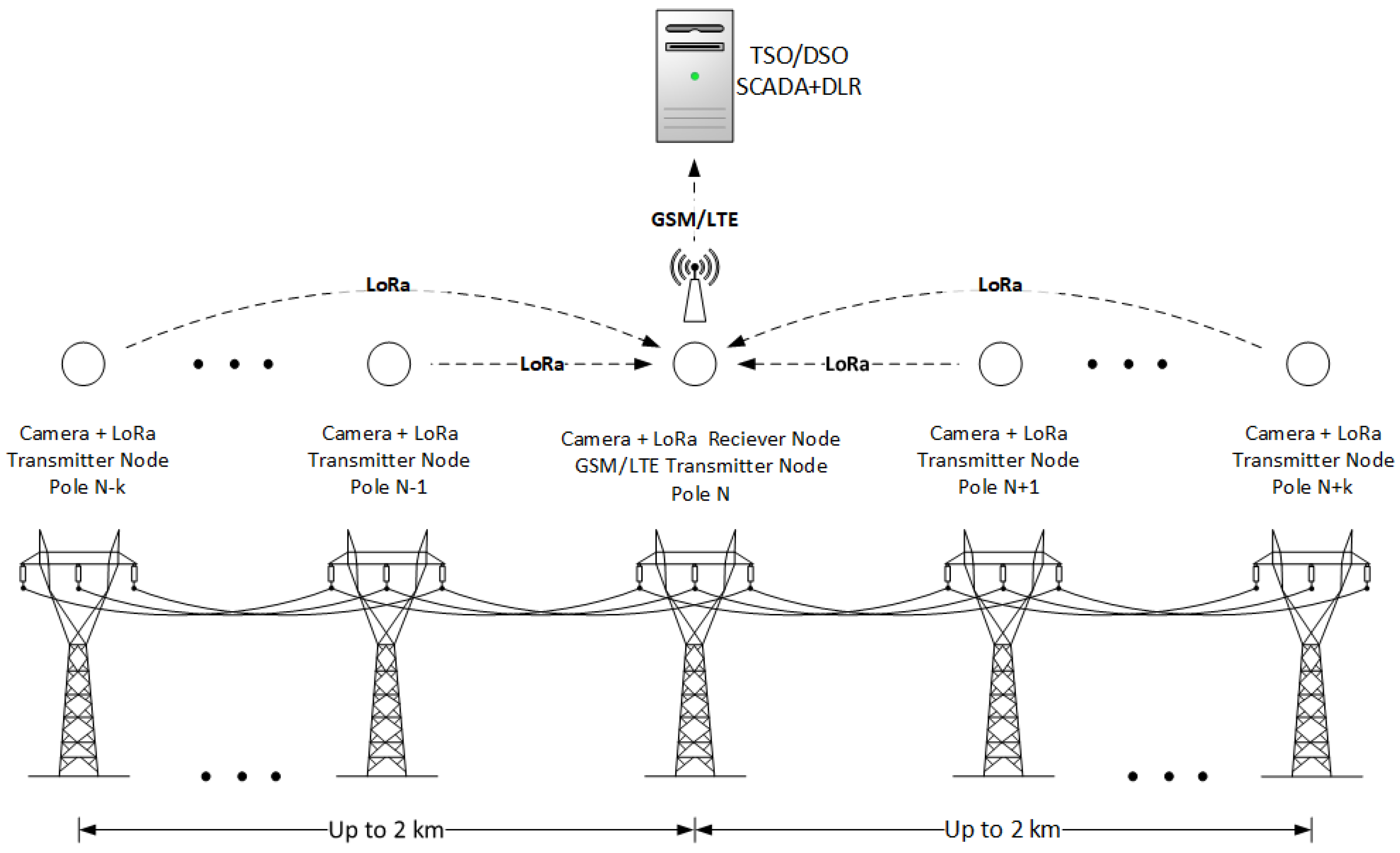
  • The communication architecture based on LoRa is proposed, and in-situ data transmission performance under 110 kV power line is investigated;
  • The proposed system for monitoring real OTL consisting of 80 poles is modeled in Automated Quality of Protection Analysis (AQoPA) and examined for overall performance.
The rest of this paper is organized in the following way: Section 2 covers the description of methods and developed system of OTL’s sag and temperature monitoring using cameras, including image processing with a sag–temperature estimation algorithm and a LoRa communication architecture. Moving on to Section 3, the results from system operation are presented, while in Section 4 the overall performance is investigated. Finally, Section 5 covers conclusions and future work.

2. The Vision System for Transmission Line Sag and Temperature Monitoring with LoRa Communication

Many DLR systems determine the OTL’s ampacity based on weather conditions, the actual current, and/or wire tension measurements. In such cases, the critical parameter is temperature and sag, which depend on the safe wire clearance from the ground or from the obstacle.

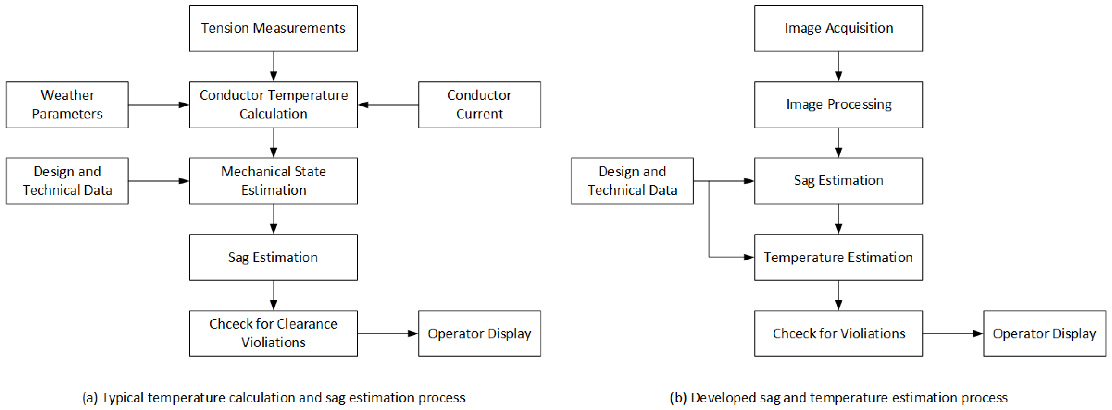
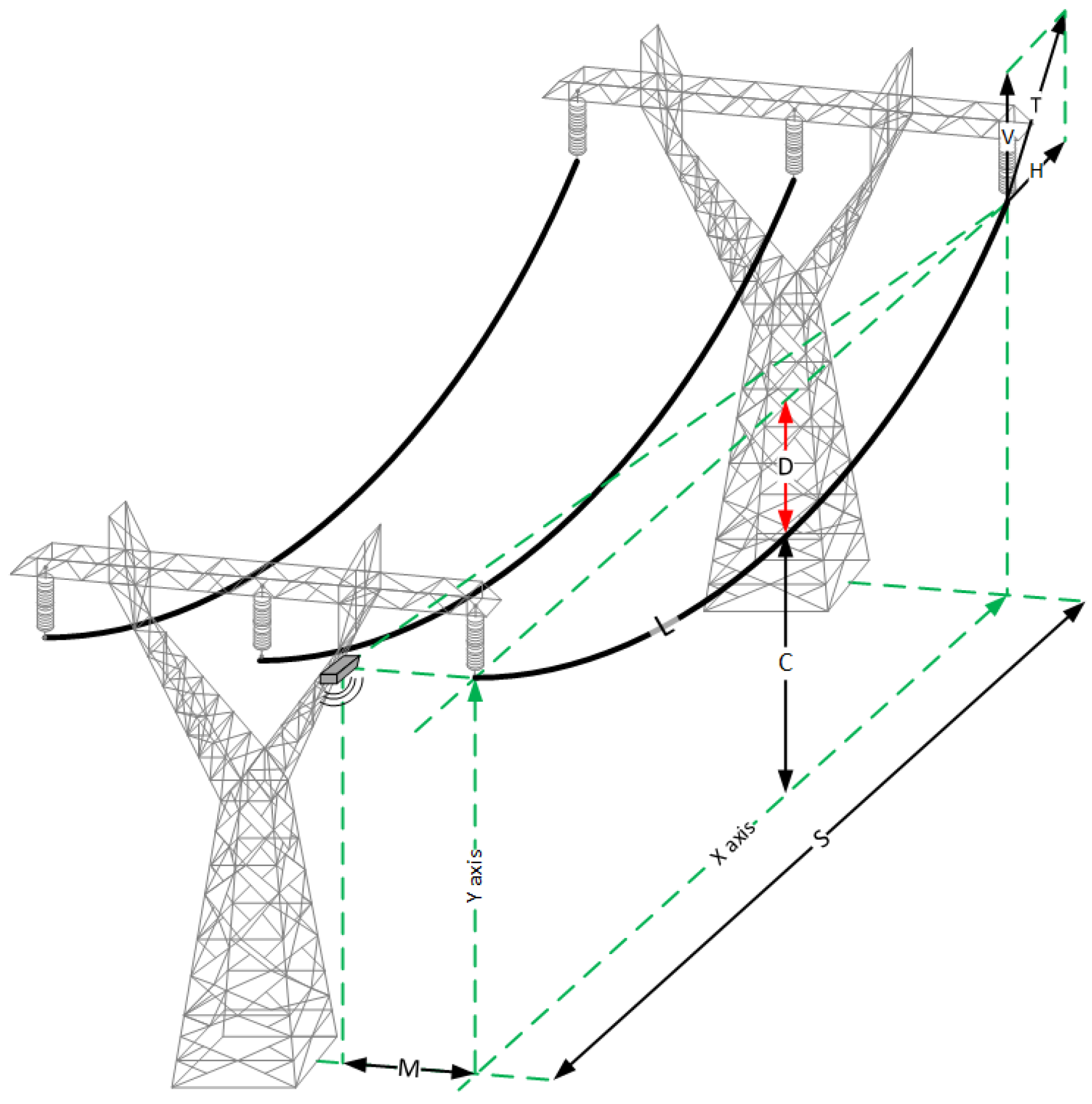
2.1. Sag–Tension Calculations of the Transmission Line Span

In mechanical overhead transmission line calculations, it is assumed that the shape of a hanging wire can be approximated by the catenary curve. The shape of a catenary is a function of the conductor weight per unit length weight w, the horizontal component of wire tension H, span length S, and the maximum sag of the conductor D. The exact catenary equation uses hyperbolic functions, as shown in Equation (1). The right side of Equation (1) is an approximation of the hyperbolic cosine using the Maclaurin series expansion:
y ( x ) = H w cosh w H x 1 = w ( x 2 ) 2 H .
For flat spans, assumed in this paper, the low point is at the center and the wire sag D is found by substituting x = S / 2 . Exact and approximate formulas for the sag calculations are shown in Equations (2) and (3):
D = H w cosh w S 2 H x 1 = w S 2 8 H
D = 3 S ( L S ) 8 .
It can be seen from Equation (3) that wire sag D depends strongly on wire length L, which varies as a function of initial conditions, temperature, and stress (4):
L 2 = α L 1 ( T 2 T 1 ) + β L 1 ( σ 2 σ 1 )
where L 1 , L 2 —initial and end state wire length; T 1 , T 2 —initial and end wire temperature; α — conductor’s thermal elongation coefficient; β —conductor’s modulus of elasticity; σ 1 , σ 2 —initial and end state conductor stress calculated as σ = H / A ; A—wire cross-sectional area.
The standard temperature–tension calculations of the power line spans are performed using Equation (5) and solved using iterative methods [15,33]:
σ 2 S 2 g 2 2 24 β σ 2 2 = σ 1 S 2 g 1 2 24 β σ 1 2 α β ( T 2 T 1 ) .
The classical method for sag calculation in power line spans presented above requires many measurements distributed along the OTL, which can be difficult to achieve. The classical method of sag–tension calculation is presented in Figure 1a [34] and compared to the proposed method in Figure 1b.
As presented in Figure 1a, the typical method of sag and temperature estimation requires the measurements of wire tension, conductor current, and actual weather parameters such as insolation, ambient temperature, and wind speed with its direction [11]. Having those values, the thermal model [35,36] calculates the actual wire temperature. The mechanical state estimation is performed by solving Equation (5) and calculating wire temperature T and strain σ , which allow for the determination of length L (4) and sag estimation D using Equation (3). In the proposed approach (Figure 1b), the wire sag D can be estimated assuming wire centenary or parabolic shape in the span in Equations (1) and (2) having known pole-span dimensions and wire parameters, combined with imagery taken by a camera as shown in Figure 2. The image is filtered and processed for final sag–temperature estimation as presented in Figure 3. Calculated wire length L using Equation (3) from sag D allows for the temperature estimation using Equations (4) and (5). In the proposed method, the wire thermal model and direct measurements from the OTL are not required.
As presented in Figure 1b, the proposed system performs wire sag–temperature calculations based on previously processed image used for the extraction of wire shape between two poles. The successive stages of span image processing are presented in Figure 3. The image processing and sag estimation algorithm (Figure 3) has been developed using Matlab/Simulink© [37] with Image Processing Toolbox [38] and implemented on Raspberry Pi 3 B+ © equipped with a camera after successful implementation of IEC61850 presented in [39]. The algorithm prototyping was possible through the use of Matlab/Simulink Hardware Support Package for Raspberry Pi 3 B+ [40], but the final standalone application was embedded on Raspberry Pi 3 B+ using Python 3.6.5 and the scikit-image library [41]. In the presented algorithm (Figure 3), Canny’s edge detection method was used [42].

2.2. Communication Architecture of the Transmission Line Sag and Temperature Monitoring System

There is now an increased interest in very promising LoRa technology, typically used for communication or data transmission in various applications [43,44,45]. Recently, the LoRa technology has been successfully implemented in the monitoring of different components in power systems such as grid [29] or Renewable Energy Sources (RES) [28,43]. The impressive range of 112 km is shown in [46]. In typical applications, LoRa can achieve a range from 2 to 15 km [47,48]. Some security issues and improvements have been identified and examined in [49,50]. Based on the research above and in [18,19,51], the power line sag–temperature communication architecture is proposed and is shown in Figure 4.
In the presented power line monitoring system, all spans’ images are processed on RPis estimating local sags and temperatures. Next, the values of wire sag and temperature with time stamps are transmitted to the sink. The sink node receives the sag–temperature data from adjacent poles of up to a 2 km distance, which typically covers from 4 to 7 poles. The calculated and transmitted sink sag–temperature values are then sent further to the operator’s SCADA system through GSM/LTE. The necessity of installing cameras on every transmission tower depends on the many factors such as geographical and weather conditions and the possibility of line overloading. Such factors are typically analyzed by operators or utility experts when deciding if all or only chosen spans need to be monitored. We chose the scenario where all spans are monitored, which ensures complete information about line operating parameters. However, in some situations, the sag–temperature monitoring nodes can be identified by operators’ critical spans, which would lower application and operational costs.

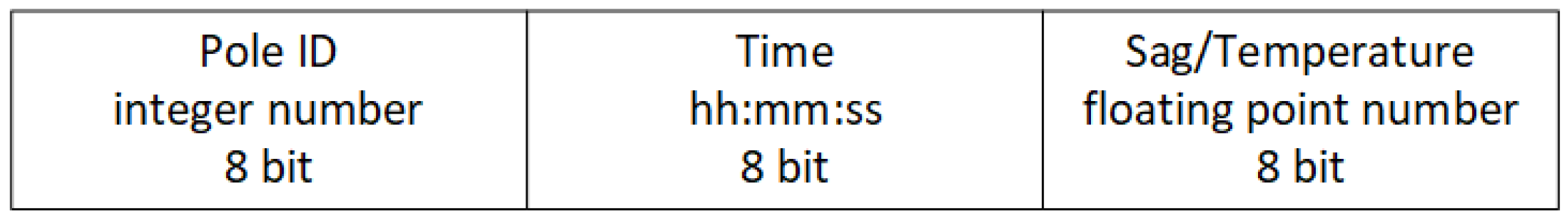
2.3. LoRa Communication Configuration

As previously mentioned, LoRa is a wireless transmission technology adapted to exchange small portions of data over long distances. The real effective range depends on terrain, ambient conditions, and used antennas [46]. In the presented system, the Pycom LoPy4 modules are used as a communication backbone. Modules are based on ESP32 development boards with an inbuilt SX1276 transceiver connected over the SPI interface. An important advantage of utilized LoPy4 modules is low-energy consumption, which requires only 25 μ A in sleep mode. This feature makes LoPy4 modules ideally suited for the developed system. During tests, the communication is configured in MAC mode (raw LoRa), which allows for bypassing the LoRaWAN layer. In such a connection type, the transmitting packet does not contain additional information such as addressing and is not formatted or encrypted by default [52]. Table 1 shows the LoRa connection settings used in the tests, where TX is the transmission power, SF is the spreading factor, BW is the bandwidth, and CR is the coding rate.
Settings presented in Table 1 are allowed for the most reliable transmission. The TX parameter has been set to the maximum possible value to achieve the required distance. The SF parameter is responsible for the duration of the chirp. The higher SF values are, the more reliable the connection is, while the lower SF values reduce the range and increase the bit rate. The spreading factor was set to 12, which is the highest possible setting. The BW parameter was set to 125 kHz. This is a measure between the upper and lower frequency of the chirp. The coding rate was set to 4/8. This parameter is connected with forward error correction. In this technique, the message contains redundant data that help detect errors. In fact, the coding rate corresponds to the proportion of bits that actually carry information. In this setting, twice as many bytes are transmitted. The transmitted data structure is presented in Figure 5.
Sending a packet of this size takes 2093 milliseconds assuming the settings shown above. It also provides all the required data to identify the measurement.

3. Results

This section covers the results achieved from the operation of the developed vision system in the flat span testbed (Figure 6), where the draw-wire displacement sensor Micro-Epsilon WDS 2500-P96 with an accuracy of ±2.5 mm was used for direct sag measurement. The horizontal tension was measured using Instron PM-L 2526-802 10 kN load cell with an accuracy of 0.5%. The wire temperature was measured with a DS18B20 sensor connected to an Arduino borad.
The single node consisting of Raspberry Pi 3B+ with a NOIR Camera and Pycom communication modules is shown in Figure 7. The Raspberry Pi board is powered with 5 V and needs approximately 610–700 mA when running Raspbian operating system and performing extensive calculations on CPU. Depending on the operating system configuration and running interfaces (e.g., HDMI, WiFi, and USB), the power consumption can be lowered to approximately 145 mA. In the proposed vision system, the sag and temperature estimation procedure is launched in a 10 min interval, where less than 25 s is needed for the image processing and sag-temperature computations. It can be assumed that, during 575 s, Raspberry Pi consumes 200 mA, and in 25 s it consumes approximately 700 mA. Based on technical data, battery capacity with a solar panel that allows for charging of the battery and powering of a Raspberry Pi equipped camera and LoRa transmitter can be designed. A similar power supply solution has been examined in [11]. Presented in Figure 4 is an RPi with a LoRa receiver additionally equipped with an LTE communication module consuming an additional 400 mA.

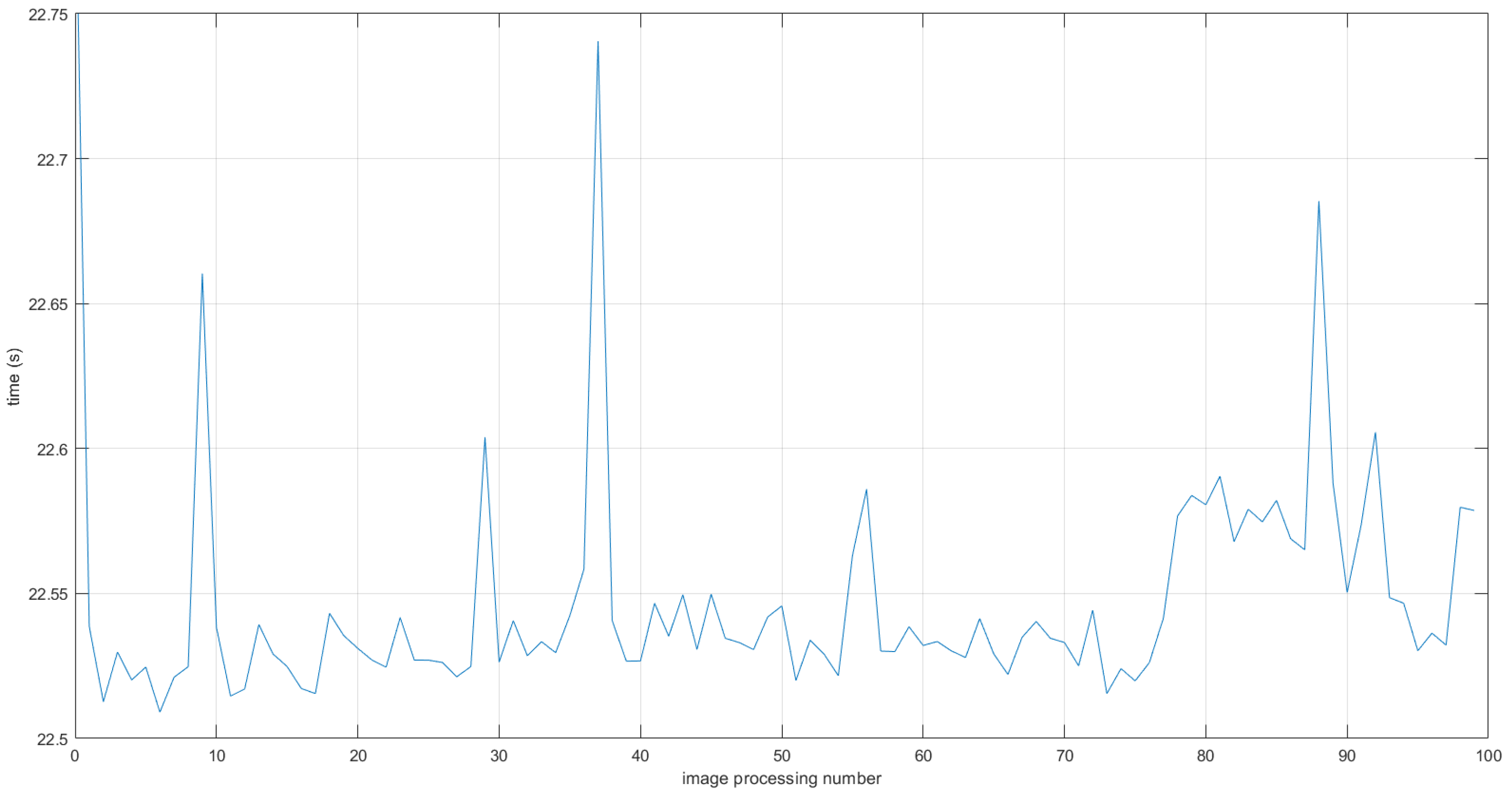
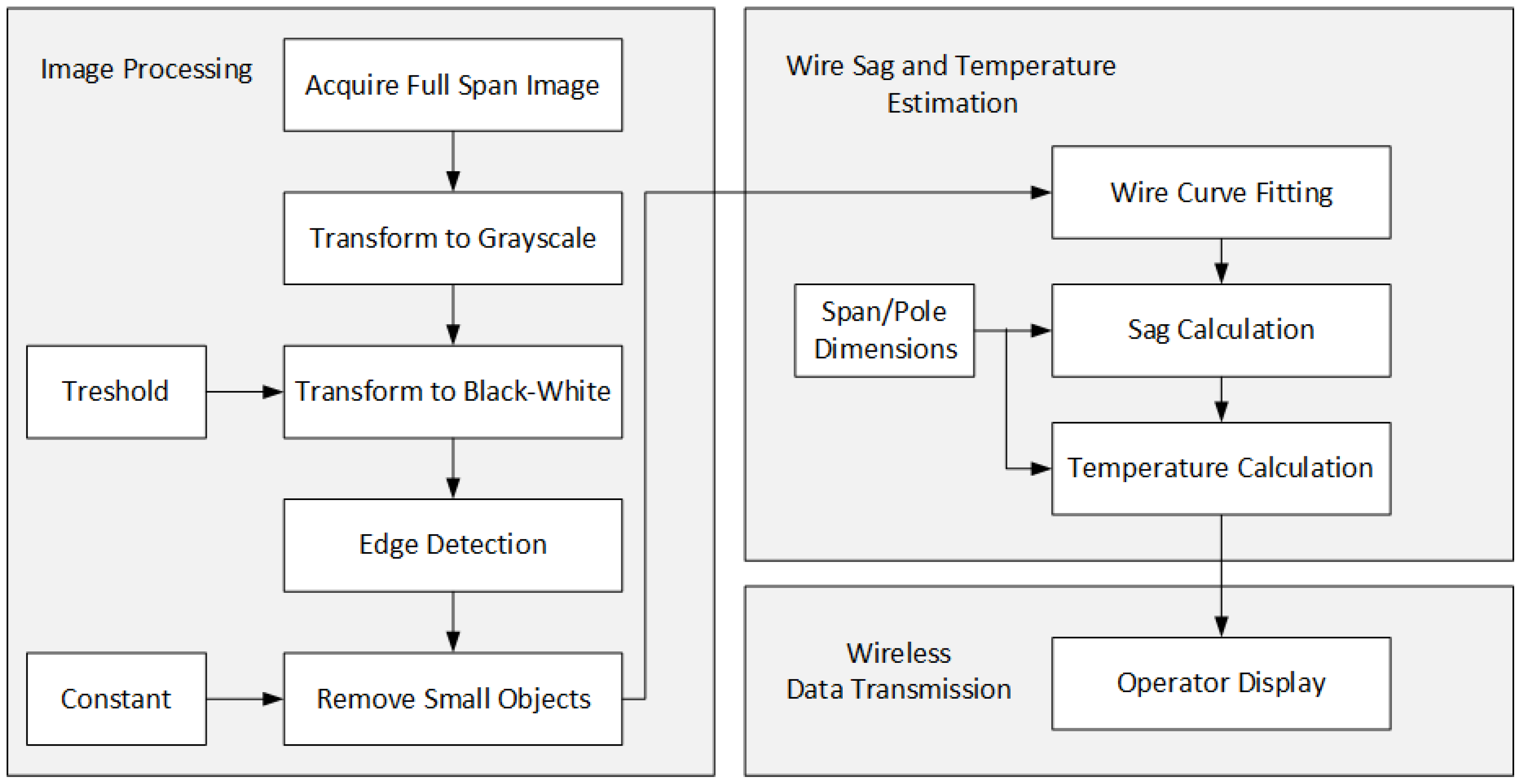
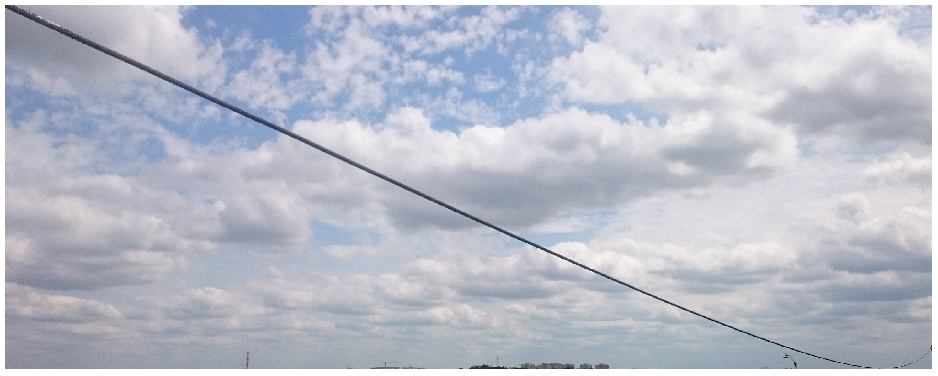
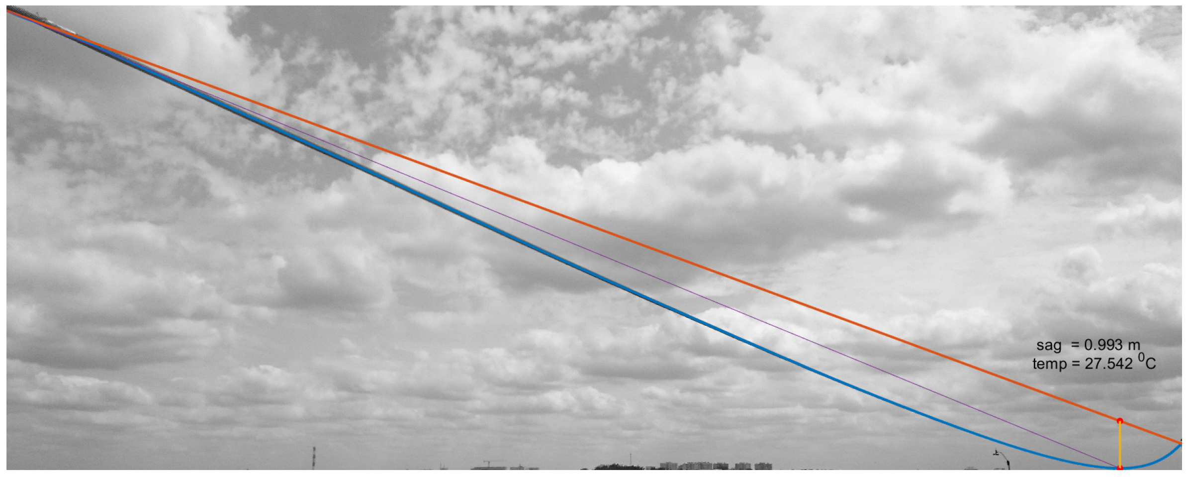
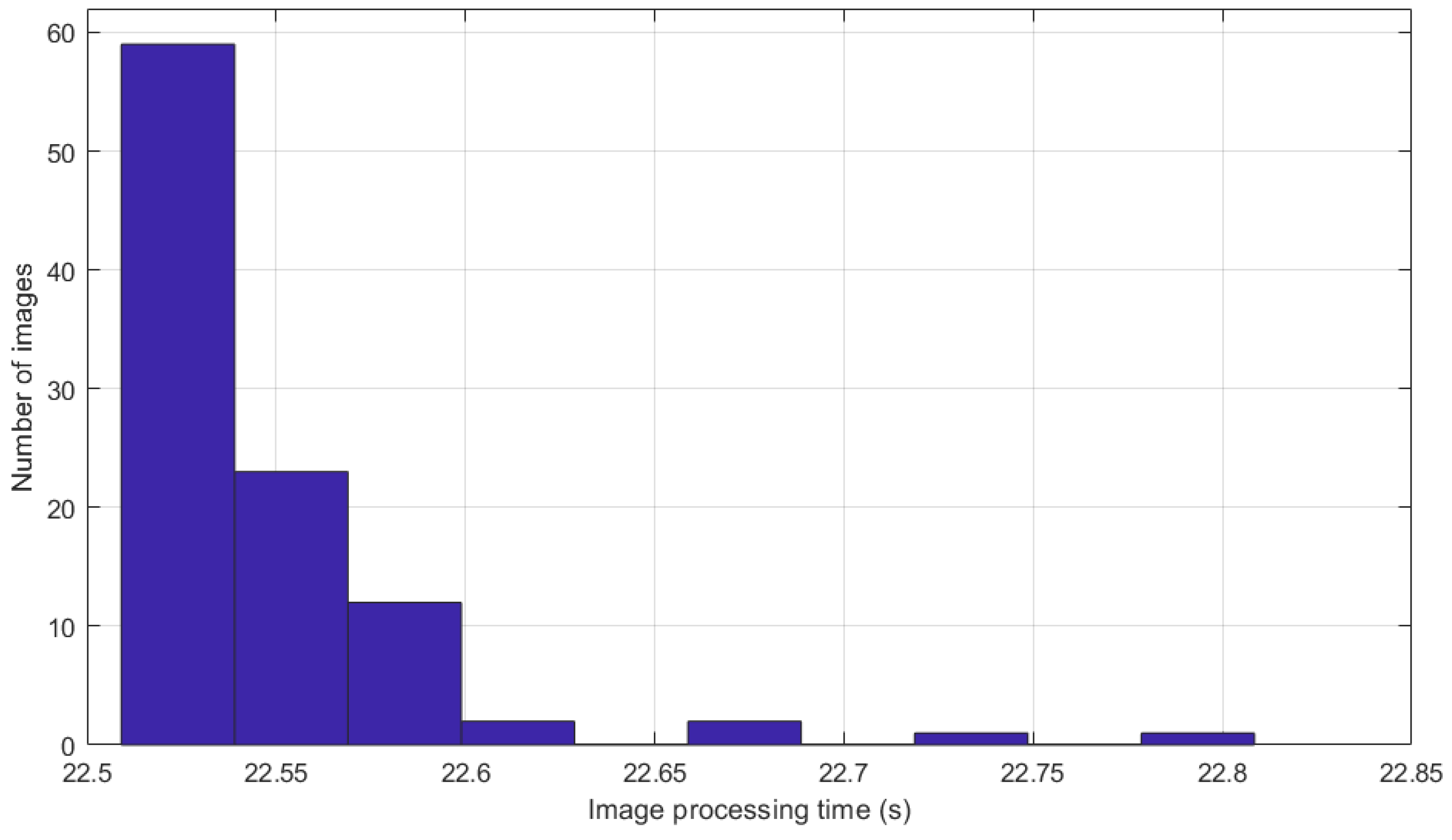
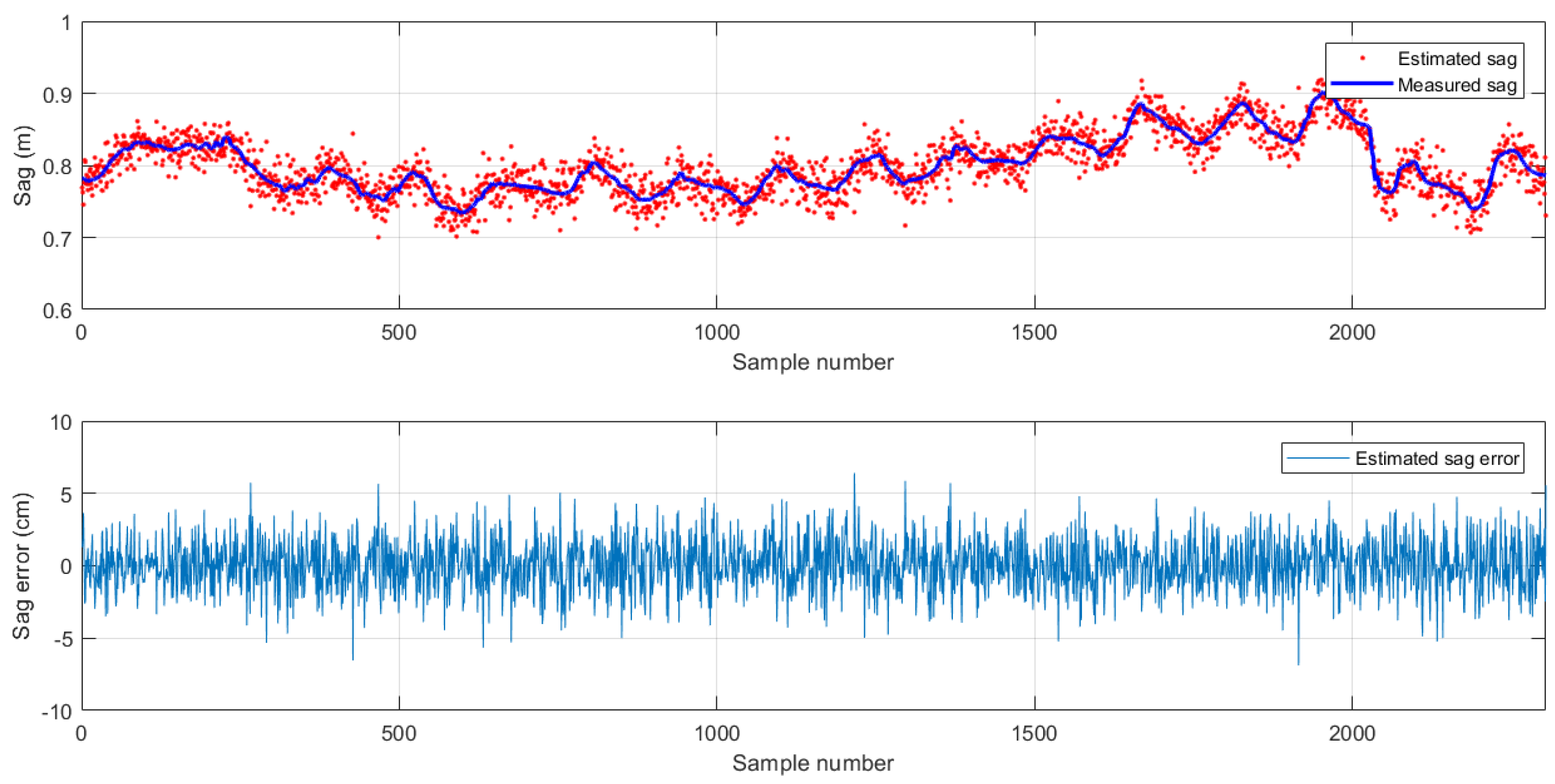
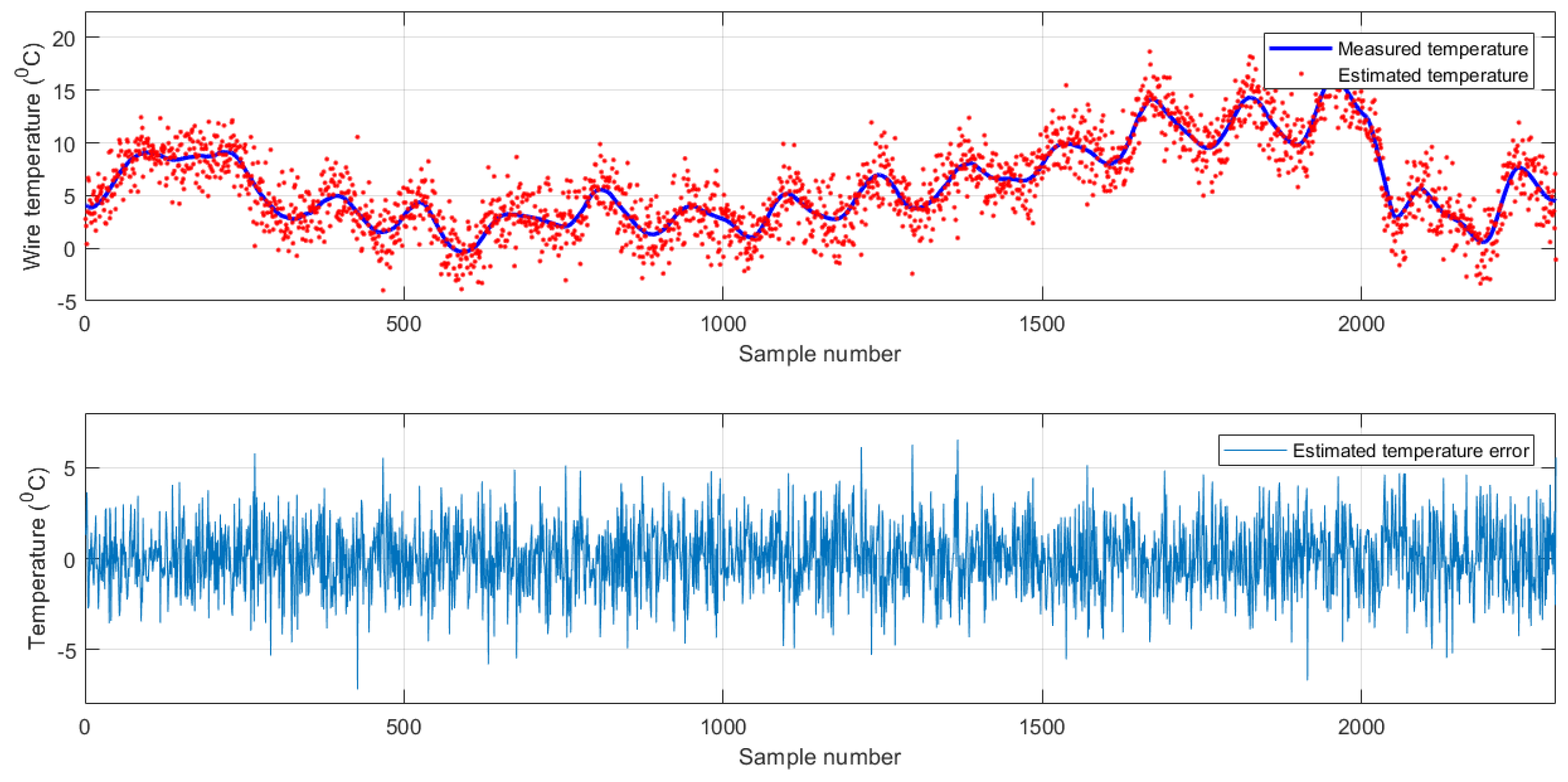
3.1. The Image Processing Algorithm for Wire Sag and Temperature Estimation

In the presented vision system, firstly, the sag of the wire is extracted from the image, and, using catenary equation, the actual wire temperature is then calculated taking the span’s technical data as input parameters. The step-by-step image processing results, according to the stages defined in Figure 3, are presented in Figure 8, Figure 9, Figure 10 and Figure 11 with the final stage and results presented in Figure 12.
The final results with estimated sag and wire temperature are presented in Figure 12 and Table 2. The parameters of ACSR 26/7 Hawk wire have been assumed to be equal, as follows: A = 276.2 mm 2 , 1 / β = 75 MPa, g = 34.47 N/(m · mm 2 ) , α = 18.7 · 10 6  1/K.
The image processing algorithm performance results, implemented in Python and embedded on Raspberry Pi 3B+, are presented in Appendix A.1, Figure A1, Figure A2, and Table 3. From the analysis of results gathered in Table 3, it can be easily observed that the mean time of a single run is 22.548 s, which has been taken for system performance modeling and simulations in AQoPA.
The results of proposed vision system operation estimating wire sag and temperature are presented in Figure 13 and Figure 14, respectively. The error statistics for sag and temperature estimation are summarized in Table 4 and Table 5.
The analysis of achieved results allows us to conclude that the standard deviation of sag estimation is ±1.8 cm in a 50 m span, while the temperature estimation standard deviation is approximately ± 1.9 C. Very promising is the mean error, varying around 0.06 cm for sag estimation and  0.05 C for temperature estimation. This shows that the presented method accuracy can be improved by performing more than one photo of the span and calculating the mean value from multiple sag and temperature estimations.

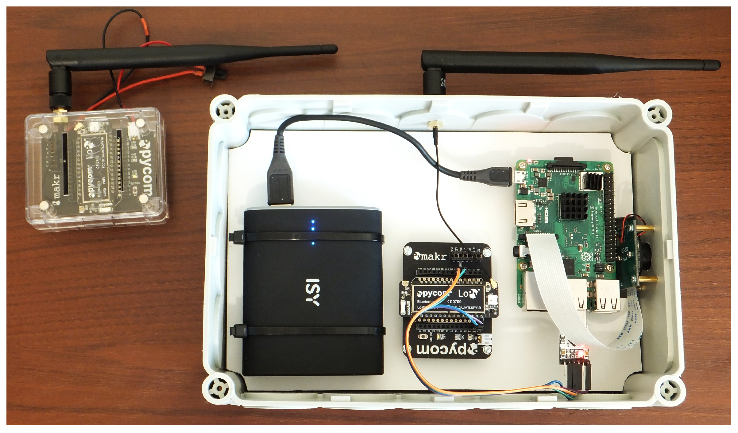
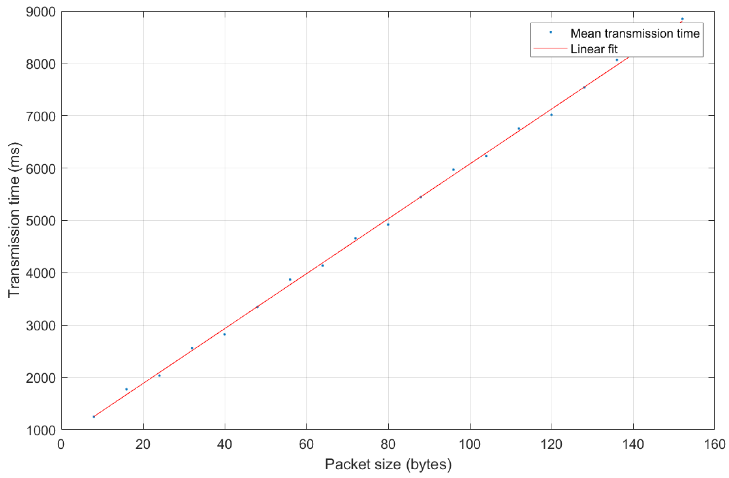
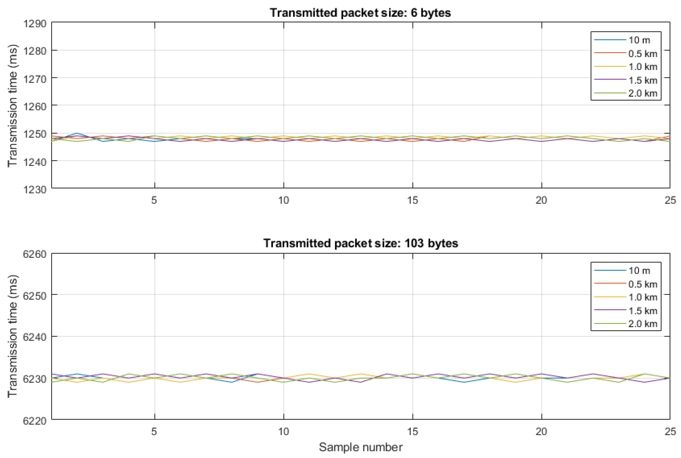
3.2. LoRa Experiment and Results

The LoRa transmission time measurements were realized on real 110 kV OTL. During the tests, a two-way connection was configured. One module sent data and waited for confirmation that the message was received. This allowed the time of data transfer to be measured. The timer started measurement when the data was sent, and stopped when confirmation was received. Each operation had a blocking status, so no other operation was performed until the confirmation signal was received or connection timed out. The achieved results are presented in Figure 15 and Figure 16. It can be easily observed that transmission time depends only on packet size. The 6 byte packet was transmitted at a maximum of 1251 ms, while a 103 byte packet was transmitted at a maximum of 6231 ms. No transmission time vs. distance dependency was observed. According to results presented in Figure 16, the data transmission time with respect to packet size dependency can be approximated by Equation (6):
y = 52.438 · x + 834.8
where y—transmission time in milliseconds (ms); x—packet size in bytes (B).

4. Modeling and Performance Analysis of the Vision System with LoRa Communication

One of the primary advantages of simulation is that it is able to provide practical feedback when designing real world systems. This allows one to determine the performance and efficiency of the system before it is actually constructed. For this reason, by using the simulation tool, the operation and overall performance of a multi-node system that will cover a typical transmission line was analyzed. Considering such a complex environment as the HV OTLs, it is reasonable to first simulate the system before actually building it. Modeling and simulation provide an important method of analysis whereby results can be easily verified, communicated, understood, and valuable by giving clear insights into such complex systems. Moreover, a simulation model can capture many more details than an analytical model, providing increased accuracy and more precise forecasting. Considering a transmission line, which consists of a significant number of poles and spans, simulation of possible monitoring solutions additionally helps save time and costs. For the purpose of determination, the vision system operation time consisting of image processing and LoRa communication, authors have used QoP-ML [53,54] and AQoPA for modeling [55]. A model of the considered vision system for whole transmission line monitoring, developed in QoP-ML, is presented and described below. Simulation results achieved using AQoPA are also analyzed and discussed. In the presented vision system, the critical parameter is the time needed to determine the whole line ampacity, achieved by the following steps: (1) take photos of all OTLs’ spans, (2) estimate sags and temperatures, and (3) transmit values to SCADA, as shown in Figure 3. The usefulness of the presented vision system strongly depends on particular data processing and transmission times, in which the vision system will be able to deliver data to the operator’s SCADA system. The total time needed to determine actual line rating strongly depends on image processing hardware with the implemented algorithm and the communication architecture [18,19,25].

4.1. The Model

In this section, all the elements prepared for creating the model of the vision system for monitoring the transmission line in QoP-ML, and the analysis results gathered using the AQoPA tool, are presented.
Analyzing the performance of the considered transmission line monitoring system, four hosts have been modeled: (1) a sensor device responsible for measurements, (2) the processing and transferring of the data to a sink device, (3) the sink device, which acts as a transmitter, sending calculated values to the third host, and (4) the headquarters or SCADA (Figure 4) in the QoP-ML model, referred to as a base station. While there is no manager in the real life deployment of the considered system, its abstraction in QoP-ML needs the manager to handle proper packet flows. The manager stores lists of sinks and sensors and knows which sensor is assigned to which sink. Its main role is to send control messages to sink nodes, in order to give them instructions regarding which sensors they should collect data from or what the best time for performing data transmission to the substation is. Sink nodes receive a list of its sensors from the manager, generate some parameters, send them to assigned motes, and wait for the collected data. After the data is collected, sensors send it to their relay node. When the relay node receives a message from each of the four sensors and the manager, it immediately starts routing to the substation. Communication ends when the base station receives packets from all the sinks that connect directly. The full model of the presented vision system, developed in QoP-ML, can be downloaded from the [56].
In Appendix A.2, Listing A1 [18], all hosts taking part in the simulation are defined. The detailed operations performed by each of them were removed for readability and will be described in greater detail separately.
The BaseStation host model is presented in Appendix A.2, Listing A2. The role of the headquarters host (SCADA) is simple: in an infinite loop (Listing A2, Line 5), it waits for the data from sinks scattered over transmission line (Listing A2, Line 7), and saves it for further processing (Listing A2, Line 9).
Next, there is the Sensor host, responsible for image processing with sag/temperature estimation and data collection. The very first instruction of the Sensor host is the image processing (Appendix A.2, Listing A3, Line 3). When this operation is finished, the Sensor waits for parameters sent by the sink (Appendix A.2 Listing A3, Line 7), in which there is an identifier (ID) of the device that acts as the relay node for this specific sensor. Further, the sensor gathers the data obtained after the image processing (Appendix A.2, Listing A3, Line 11) and sends the data to its sink (Appendix A.2, Listing A3, Lines 17–18).
The main role of the Sink device is to gather the data obtained by its sensors: when all motes finish image processing and data gathering, they send the obtained data to the SCADA system by means of LTE. As can be seen in Appendix A.2, Listing A4, the sink consists of three processes, namely Main, WaitForData, and Communication, where each of them is in charge of different operations. The Main process (Appendix A.2, Listing A4, Lines 5–21) waits for data from the Manager, in order to receive the list of sensors, from which the sink needs to gather the data. After receiving the list of sensors, the sink generates parameters and sends them to sensor devices. The actual data gathering takes place in the WaitForData process (Appendix A.2, Listing A4, Lines 24–39), in which the sink node waits for data gathered by sensors. The Sink saves the data and adds it to the list of the collected packets. The Communication process is responsible for the actual data transmission toward the base station. Its role is to receive the initial data from the manager or another sink within its cluster. The sink adds the data to the list of the gathered packets containing image processing information and performs the routing algorithm, in order to find the path to headquarters. The Communication process ends when packets from all sinks reach the base station. Last but not least, the Manager represents a host that is not available (and not needed) in real-life deployment. As brought up earlier, its role is to work only as a helper host, which manages packet flows in our simulation. For this reason, its code is omitted.
In order to demonstrate the described behavior of the hosts taking part in model, one of the QoP-ML’s features that allow one to specify operations performed by hosts (called functions) was used. All actions taken by each of the hosts were able to be defined as measurements—image processing with sag/temperature estimation and data transmission.
Lines 3–7 presented in Appendix A.2, Listing A5, contain a declaration of functions, that are used by the Manager host to handle the division of sensors to proper sinks. Functions representing types of messages traversing the transmission line are defined in Lines 9–17 in Appendix A.2, Listing A5. Remaining functions (Appendix A.2, Listing A5, Lines 19–22) refer to data collection and are fairly self-explanatory.
Regarding the data transmission, three communication channels were modeled (one of them being the main communication channel, and two remaining needed by the model itself for communication synchronization) as presented in Appendix A.2, Listing A6. The modeled communication channel has physical characteristics defined by the LoRa digital wireless data communication technology standard. The mentioned standard was chosen because it enables very-long-range transmissions with low power consumption, which is the crucial feature when it comes to sensor devices.
The simulation begins at sensor nodes, where image processing takes place. Calculated values are sent to sink devices (also known as gateways) using the LoRa communication standard. Further, every gateway across the transmission line transfers gathered data to the operator’s SCADA system using the GSM/LTE network.

4.2. Scenarios

Analyzing monitoring of an overhead transmission line in QoP-ML, we proposed to consider a scenario that consists of 80 sensors, 10 sinks, and a single SCADA station. As can be seen, utilized hosts use metrics defined for TelosB motes (which in fact means they have its physical characteristics), while the sink node utilizes metrics for a MicaZ device (Appendix A.2, Listing A7, Lines 5–8). Further, the actual number of devices taking part in simulation is given (in curly brackets), and finally hosts are started (Appendix A.2, Listing A7, Lines 10–27). During the startup process, one can choose which processes and subprocesses defined in a model should also be launched. For instance, looking at the Sink host defined earlier in our model, it can be seen that it has three processes and three subprocesses, and all of them are being started. When devices are set up and ready, communication details are defined. This can be done inside the Communication structure, where one can specify a medium’s physical characteristics (Appendix A.2, Listing A7, Lines 32–35) and the topology of the considered environment (Appendix A.2, Listing A7, Lines 36–62). With respect to the time taken for data transmission, we utilized the ( 6 ) formula. In our simulation, we assumed the packet size to be equal to 6 bytes, and used the resulting value to define the time needed by sensors sending the data to their sinks (Appendix A.2, Listing A7, Line 62).

Results and Analysis

Table 6 consists of the results gathered after the simulation of the transmission line scenario prepared in QoP-ML. In this scenario, there are 80 poles and 10 sinks. Devices are grouped such that 8 poles send data to their sink, which further transmits it to SCADA system. There are 10 groups, each of them consisting of 1 sink and 8 sensors. (Sensors 1-8 and Sink 1 are the first group, Sensors 9–16 and Snk 2 are the second, and so on.)
As can be seen in Table 6, the transmission time between sensor and their sink is different for each mote within a group. It results from the fact that data transmitted from sensors is being queued at the sink’s side, while every sensor performs image processing at the same time and sends gathered data immediately to its sink. The time in which the SCADA system is given full information from all of the 80 poles is the maximum time from 8 groups, which is equal to 48.47 s.

5. Conclusions

There are many DLR systems that allow for the calculation of the actual OTL’s ampacity. The main drawback of most currently used methods is the necessity of sensor installation directly on OTLs’ wires, which implies a switching off the line from operation. In this paper, the concept of a contactless vision system for monitoring OTL’s wire sag and temperature with LoRa communication (used for data transmission) is presented. The single span sensor node equipped with a camera and LoRa communication was built. The algorithm for OTL’s wire sag and temperature estimation was developed, implemented, and tested in a 50 m long test span with an ACSR Hawk 26/7 wire. The presented technique estimation accuracy for a wider range of sags and temperatures using high currents has been scheduled as the next research step. The final stage will be the installation of the presented vision system on an in-service high voltage OTL. The LoRa communication has been tested under in-service 110 kV OTL, proving (1) the correctness of LoRa settings assumed, (2) the operational range, and (3) the transmission time. The overall performance of the proposed vision system monitoring 80 km OTL was evaluated using developed models in QoP-ML and analyzed with the AQoPA tool. The system performance results proved that the longest data transmission time was less than 48.5 s, while the standard OTL’s wire time constant is assumed to be within 5–15 min (300–900 s). The simple comparison of times shows that the overall vision system performance is from almost 6.2 to 18.55 times higher than the standard wire time constant, which proves the system’ applicability and usability. In the proposed topology, 80 poles OTL can be fully monitored in less than 50 s. The total time, which is needed to determine the actual line rating can be shortened using more efficient processor boards or smart-cameras with built-in image processing algorithms on FPGAs. The presented system can be also expanded with further algorithms, e.g., for ice detection, which would improve its future functionality. The usage of FLIR cameras, smart cameras, and encryption for data transmission security, as well as an investigation of a system’s lifetime and reliability with LoRa communication, will be topics of future work.

Author Contributions

M.W. and B.K. contributed to the idea of this work. M.W. contributed the parts concerning the dynamic line rating, the idea of the vision system, and the method of wire sag–temperature estimation with its practical implementation and performance testing. M.W. and P.K. practically developed the prototype. P.K. implemented and tested the LoRa communication under HV transmission line, and M.W. with B.K. analyzed the results. K.M. created the model for system performance analysis, performed simulations, and gathered results. M.W. wrote most of the article, and edited the final paper. M.W. and B.K. organized the work, defined and supervised the research, and were involved in structuring the paper. M.W. organized the funding. All authors contributed to the discussion of the results and the reviewing process of the intellectual content of the article and finally approved the manuscript.

Funding

This research received no external funding.

Conflicts of Interest

The authors declare no conflict of interest.

Abbreviations

The following abbreviations are used in this manuscript:
WSNWireless Sensor Network
DLRDynamic Line Rating
ICTsInformation and Communication Technologies
CPUCentral Processing Unit
PSPower System
SEState Estimation
OTLOverhead Transmission Line
QoP-MLQuality of Protection Modeling Language
AQoPAAutomated Quality of Protection Analysis
SCADASupervisory Control And Data Acquisition
RESRenewable Energy Sources
LoRaLong Range
CNNConvolutional Neural Network
IEDIntelligent Electronic Device

Appendix A

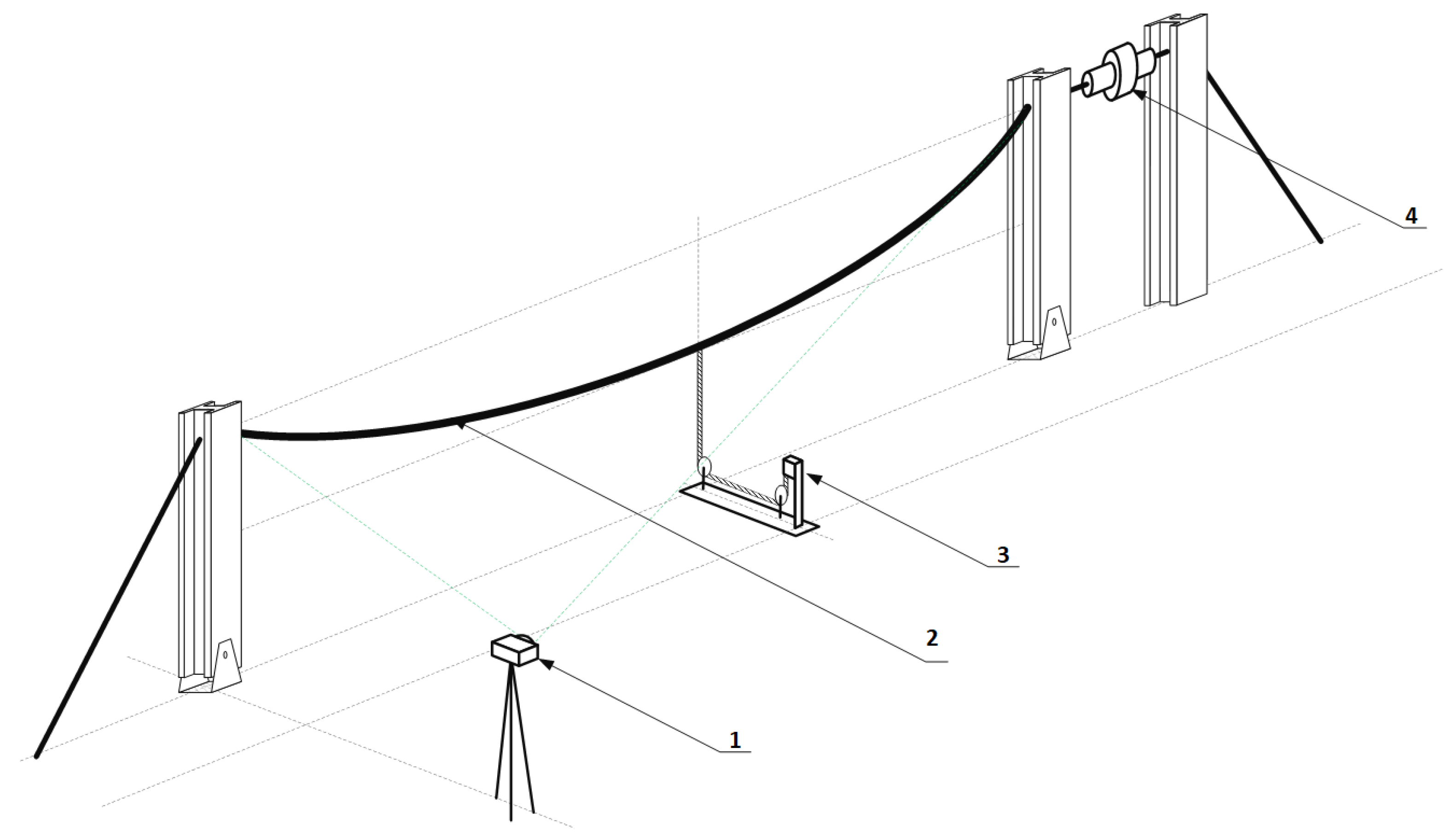
Appendix A.1. Single Span Image Processing and Sag Estimation

Figure A1. Image processing with sag estimation algorithm performance running on Raspberry Pi 3 B+.
Energies 12 00505 g0a1
Figure A2. Histogram of algorithm performance running on Raspberry Pi 3 B+.
Energies 12 00505 g0a2

Appendix A.2. QoP-ML Listings

Listing A1. QoP-ML’s hosts taking part in simulation.
  
hosts1
{2
host BaseStation(rr)(*) { ... }3
host Sensor(rr)(*) { ... }4
host Sink(rr)(*) { ... }5
host Manager(fifo)(*) { ... }6
}7
  
Listing A2. The headquarters host implemented in QoP-ML.
  
host BaseStation(rr)(*)1
{2
process Main(*)3
{4
while(true)5
{6
in(ch_WSN: DATA_MSG: |*, id(), sink_data_msg()|);7
bsDATA = DATA_MSG[3];8
save_collected_data(bsDATA)[UPDATED];9
}10
}11
}12
  
Listing A3. The sensor host implemented in QoP-ML.
  
host Sensor(rr)(*)1
{2
# img = process_image();3
4
process Main(*)5
{6
in(ch_WSN: PARAMS_MSG: |*, id(), params_msg()|);7
PARAMS = PARAMS_MSG[3];8
SINK_ID = PARAMS_MSG[0];9
10
GATHERED_DATA = collected_data()[UPDATED];11
save_collected_data(GATHERED_DATA)[UPDATED];12
13
COLLECTED_NOTIFICATION_MSG = (id(), broadcast(), data_collected_msg());14
out(ch_MGNT: COLLECTED_NOTIFICATION_MSG);15
16
DATA_MSG = (id(), SINK_ID, data_msg(), GATHERED_DATA);17
out(ch_WSN: DATA_MSG);18
}19
}20
  
Listing A4. The sink host implemented in QoP-ML.
  
host Sink(rr)(*)1
{2
# COLLECTED_DATA = empty_list();3
4
process Main(*)5
{6
in(ch_MGNT: NODES_MSG: |*, id(), nodes_msg()|);7
NODES_LIST = NODES_MSG[3];8
9
TMP_NODES_LIST = NODES_LIST;10
11
while (is_list_empty(TMP_NODES_LIST) != true) {12
13
PARAMS = generate_params();14
15
NODE_ID = get_from_list(TMP_NODES_LIST);16
TMP_NODES_LIST = pop_list(TMP_NODES_LIST);17
18
PARAMS_MSG = (id(), NODE_ID, params_msg(), PARAMS);19
out(ch_WSN: PARAMS_MSG);20
}21
}22
23
process WaitForData(*) {24
25
in(ch_MGNT: NODES_MSG2: |*, id(), nodes_msg()|);26
TMP_NODES_LIST2 = NODES_MSG2[3];27
28
while (is_list_empty(TMP_NODES_LIST2) != true) {29
30
in(ch_WSN: DATA_MSG_FROM_SENSORS: |*, id(), data_msg()|);31
DATA_FROM_SENSORS = DATA_MSG_FROM_SENSORS[3];32
33
save_collected_data(DATA_FROM_SENSORS)[UPDATED];34
COLLECTED_DATA = add_to_list(COLLECTED_DATA, DATA_FROM_SENSORS);35
36
TMP_NODES_LIST2 = pop_list(TMP_NODES_LIST2);37
}38
}39
40
process HopByHopComm(*)41
{42
in(ch_WSN: SINK_DATA_MSG: |*, id(), sink_data_msg()|);43
DATA_FROM_SINK = SINK_DATA_MSG[3];44
COLLECTED_DATA2 = add_to_list(COLLECTED_DATA, DATA_FROM_SINK);45
46
NEXT_HOP_ID = routing_next(wsn, id(BaseStation.0));47
DATA_MSG = (id(), NEXT_HOP_ID, sink_data_msg(), COLLECTED_DATA2);48
out(ch_WSN: DATA_MSG);49
}50
51
}52
  
Listing A5. QoP-ML’s functions prepared for a transmission grid model.
  
functions1
{2
fun empty_list();3
fun add_to_list(list, element);4
fun get_from_list(list);5
fun pop_list(list);6
fun is_list_empty(list);7
8
fun nodes_msg();9
fun sinks_msg();10
fun params_msg();11
fun start_sensing_msg();12
fun start_collecting_msg();13
fun data_collected_msg();14
fun data_req_msg();15
fun data_msg();16
fun empty(); 17
18
fun process_image();19
fun generate_params(node_id);20
fun collected_data();21
fun save_collected_data(data);22
}23
  
Listing A6. QoP-ML’s communication channels prepared for a transmission grid model.
  
channels1
{2
channel ch_WSN(*)[wsn];3
channel ch_MGNT(*)[mgnt];4
channel ch_TIMER(*)[timer];5
}6
  
Listing A7. Transmission line scenario.
  
versions1
{2
version TransmissionLine3
{4
set host Sink(MicaZ);5
set host Sensor(TelosB);6
set host BaseStation(TelosB);7
set host Manager(TelosB);8
9
run host Sink(*){10} {10
run Main()11
run WaitForData()12
run Communication()13
}14
15
run host Sensor(*){80} {16
run Main()17
}18
19
run host Manager(*) {20
run PrepareMessages(*)21
run Main()22
}23
24
run host BaseStation(*) {25
run Main()26
}27
28
communication {29
medium[wsn] {30
default_q = 1;31
default_time = wsn_time [ms];32
default_listening_current = 1.14 mA;33
default_sending_current = 22.8 mA;34
default_receiving_current = 22.8 mA;35
topology {36
37
Manager -> Sink[0:9] : time = 0 ms;38
39
Sink[0] <-> Sensor[0:7] : time = 1149.428ms;40
Sink[1] <-> Sensor[8:15] : time = 1149.428ms;41
Sink[2] <-> Sensor[16:23] : time = 1149.428ms;42
Sink[3] <-> Sensor[24:31] : time = 1149.428ms;43
Sink[4] <-> Sensor[32:39] : time = 1149.428ms;44
Sink[5] <-> Sensor[40:47] : time = 1149.428ms;45
Sink[6] <-> Sensor[48:55] : time = 1149.428ms;46
Sink[7] <-> Sensor[56:63] : time = 1149.428ms;47
Sink[8] <-> Sensor[64:71] : time = 1149.428ms;48
Sink[9] <-> Sensor[72:79] : time = 1149.428ms;49
50
Sink[0] -> BaseStation[0];51
Sink[1] -> BaseStation[0];52
Sink[2] -> BaseStation[0];53
Sink[3] -> BaseStation[0];54
Sink[4] -> BaseStation[0];55
Sink[5] -> BaseStation[0];56
Sink[6] -> BaseStation[0];57
Sink[7] -> BaseStation[0];58
Sink[8] -> BaseStation[0];59
Sink[9] -> BaseStation[0];60
}61
} %62
63
medium[mgnt] {64
default_q = 1;65
default_time = 0ms;66
default_listening_current = 0mA;67
default_sending_current = 0 mA;68
default_receiving_current = 0 mA;69
70
topology {71
Manager -> Sink[0:9]: time = 0 ms;72
Manager <-> Sensor[0:79];73
Sink[0] <-> Sensor[0:7];74
Sink[1] <-> Sensor[8:15];75
Sink[2] <-> Sensor[16:23];76
Sink[3] <-> Sensor[24:31];77
Sink[4] <-> Sensor[32:39];78
Sink[5] <-> Sensor[40:47];79
Sink[6] <-> Sensor[48:55];80
Sink[7] <-> Sensor[56:63];81
Sink[8] <-> Sensor[64:71];82
Sink[9] <-> Sensor[72:79];83
}84
}85
}86
}87
}88
  

References

  1. Murphy, S.; Niebur, D. Real-time monitoring of transmission line thermal parameters: A literature review. In Proceedings of the 2018 IEEE Power Energy Society Innovative Smart Grid Technologies Conference (ISGT), Washington, DC, USA, 19–22 February 2018; pp. 1–5. [Google Scholar] [CrossRef]
  2. Akpolat, A.N.; Nese, S.V.; Dursun, E. Towards to smart grid: Dynamic line rating. In Proceedings of the 2018 6th International Istanbul Smart Grids and Cities Congress and Fair (ICSG), Istanbul, Turkey, 25–26 April 2018; pp. 96–100. [Google Scholar] [CrossRef]
  3. Douglass, D.; Chisholm, W.; Davidson, G.; Grant, I.; Lindsey, K.; Lancaster, M.; Lawry, D.; McCarthy, T.; Nascimento, C.; Pasha, M.; et al. Real-Time Overhead Transmission-Line Monitoring for Dynamic Rating. IEEE Trans. Power Deliv. 2016, 31, 921–927. [Google Scholar] [CrossRef]
  4. Moldoveanu, C.; Rusu, A.; Florea, M.; Vaju, M.; Hategan, I.; Iacobici, L.; Balta, N.; Zaharescu, S.; Avramescu, M.; Curiac, P.; et al. OHLM: Integrated solution for real-time monitoring of overhead transmission lines. In Proceedings of the 2016 IEEE PES 13th International Conference on Transmission Distribution Construction, Operation Live-Line Maintenance (ESMO), Columbus, OH, USA, 12–15 September 2016; pp. 1–5. [Google Scholar] [CrossRef]
  5. Aznarte, J.L.; Siebert, N. Dynamic Line Rating Using Numerical Weather Predictions and Machine Learning: A Case Study. IEEE Trans. Power Deliv. 2017, 32, 335–343. [Google Scholar] [CrossRef]
  6. Bhattarai, B.P.; Gentle, J.P.; McJunkin, T.; Hill, P.J.; Myers, K.; Abboud, A.; Renwick, R.; Hengst, D. Improvement of Transmission Line Ampacity Utilization by Weather-Based Dynamic Line Ratings. IEEE Trans. Power Deliv. 2018, 33, 1853–1863. [Google Scholar] [CrossRef]
  7. Guo, R.; Zhang, F.; Zhong, L. Intelligent on-line monitoring system based on elastic wave for overhead transmission lines. In Proceedings of the 2013 IEEE International Conference on Information and Automation (ICIA), Yinchuan, China, 26–28 August 2013; pp. 115–118. [Google Scholar] [CrossRef]
  8. Wydra, M.; Kacejko, P. Power system state estimation using wire temperature measurements for model accuracy enhancement. In Proceedings of the 2016 IEEE PES Innovative Smart Grid Technologies Conference Europe (ISGT-Europe), Ljubljana, Slovenia, 9–12 October 2016; pp. 1–6. [Google Scholar] [CrossRef]
  9. Wydra, M.; Kacejko, P. Power System State Estimation Accuracy Enhancement Using Temperature Measurements of Overhead Line Conductors. Metrol. Meas. Syst. 2016, 23, 183–192. [Google Scholar] [CrossRef]
  10. Wydra, M.; Kacejko, P.; Gastolek, P. The Impact of the Power Line Conductors Temperature on the Optimal Solution of Generation Distribution in the Power System. In Proceedings of the 2018 15th International Conference on the European Energy Market (EEM), Lodz, Poland, 27–29 June 2018; pp. 1–5. [Google Scholar] [CrossRef]
  11. Kacejko, P.; Wydra, M.; Nowak, W.; Szpyra, W. Advantages, Benefits, and Effectiveness Resulting from the Application of the Dynamic Management of Transmission Line Capacities. In Proceedings of the 2018 15th International Conference on the European Energy Market (EEM), Lodz, Poland, 27–29 June 2018; pp. 1–5. [Google Scholar] [CrossRef]
  12. Esfahani, M.M.; Yousefi, G.R. Real Time Congestion Management in Power Systems Considering Quasi-Dynamic Thermal Rating and Congestion Clearing Time. IEEE Trans. Ind. Inform. 2016, 12, 745–754. [Google Scholar] [CrossRef]
  13. Lovrenčić, V.; Gabrovšek, M.; Kovač, M.; Gubeljak, N.; Šojat, Z.; Klobas, Z. The Contribution of Conductor Temperature and Sag Monitoring to Increased Ampacities of Overhead Lines (OHLs). Period. Polytech. Electr. Eng. Comput. Sci. 2015, 59, 70–77. [Google Scholar] [CrossRef]
  14. de Nazare, F.V.B.; Werneck, M.M. Hybrid Optoelectronic Sensor for Current and Temperature Monitoring in Overhead Transmission Lines. IEEE Sens. J. 2012, 12, 1193–1194. [Google Scholar] [CrossRef]
  15. Wydra, M.; Kisala, P.; Harasim, D.; Kacejko, P. Overhead Transmission Line Sag Estimation Using a Simple Optomechanical System with Chirped Fiber Bragg Gratings. Part 1: Preliminary Measurements. Sensors 2018, 18, 309. [Google Scholar] [CrossRef]
  16. Ma, G.M.; Li, C.R.; Quan, J.T.; Jiang, J.; Cheng, Y.C. A Fiber Bragg Grating Tension and Tilt Sensor Applied to Icing Monitoring on Overhead Transmission Lines. IEEE Trans. Power Deliv. 2011, 26, 2163–2170. [Google Scholar] [CrossRef]
  17. Gubeljak, N.; Banić, B.; Lovrenčić, V.; Kovač, M.; Nikolovski, S. Preventing Transmission Line damage caused by ice with smart on-line conductor Monitoring. In Proceedings of the 2016 International Conference on Smart Systems and Technologies (SST), Osijek, Croatia, 12–14 October 2016; pp. 155–163. [Google Scholar] [CrossRef]
  18. Mazur, K.; Wydra, M.; Ksiezopolski, B. Secure and Time-Aware Communication of Wireless Sensors Monitoring Overhead Transmission Lines. Sensors 2017, 17, 1610. [Google Scholar] [CrossRef]
  19. Hung, K.S.; Lee, W.K.; Li, V.O.K.; Lui, K.S.; Pong, P.W.T.; Wong, K.K.Y.; Yang, G.H.; Zhong, J. On Wireless Sensors Communication for Overhead Transmission Line Monitoring in Power Delivery Systems. In Proceedings of the 2010 First IEEE International Conference on Smart Grid Communications, Gaithersburg, MD, USA, 4–6 October 2010; pp. 309–314. [Google Scholar] [CrossRef]
  20. Khawaja, A.H.; Huang, Q.; Khan, Z.H. Monitoring of Overhead Transmission Lines: A Review from the Perspective of Contactless Technologies. Sens. Imaging 2017, 18, 24. [Google Scholar] [CrossRef]
  21. Sun, X.; Huang, Q.; Hou, Y.; Jiang, L.; Pong, P.W.T. Noncontact Operation-State Monitoring Technology Based on Magnetic-Field Sensing for Overhead High-Voltage Transmission Lines. IEEE Trans. Power Deliv. 2013, 28, 2145–2153. [Google Scholar] [CrossRef]
  22. Nie, S.; Qu, G.; Ye, H.; Jiang, X. On-line monitoring system for icing state of overhead transmission line. In Proceedings of the 2012 Power Engineering and Automation Conference, Wuhan, China, 18–20 September 2012; pp. 1–5. [Google Scholar] [CrossRef]
  23. Phillips, A. Evaluation of Instrumentation and Dynamic Thermal Ratings for Overhead Lines; USDOE/EPRI/NYPA Technical Report; New York Power Authority: White Plains, NY, USA, 2013; Volume 1. [Google Scholar] [CrossRef]
  24. Cho, C.J.; Ko, H. Video-Based Dynamic Stagger Measurement of Railway Overhead Power Lines Using Rotation-Invariant Feature Matching. IEEE Trans. Intell. Transp. Syst. 2015, 16, 1294–1304. [Google Scholar] [CrossRef]
  25. Wu, Y.C.; Cheung, L.F.; Lui, K.S.; Pong, P.W.T. Efficient Communication of Sensors Monitoring Overhead Transmission Lines. IEEE Trans. Smart Grid 2012, 3, 1130–1136. [Google Scholar] [CrossRef]
  26. Fateh, B.; Govindarasu, M.; Ajjarapu, V. Wireless Network Design for Transmission Line Monitoring in Smart Grid. IEEE Trans. Smart Grid 2013, 4, 1076–1086. [Google Scholar] [CrossRef]
  27. Li, M.; Chi, X.B.; Jia, X.C.; Zhang, J.L. WSN-based efficient monitoring for overhead transmission line in smart grid. In Proceedings of the 2016 35th Chinese Control Conference (CCC), Chengdu, China, 27–29 July 2016; pp. 8485–8489. [Google Scholar] [CrossRef]
  28. Choi, C.; Jeong, J.; Lee, I.; Park, W. LoRa based renewable energy monitoring system with open IoT platform. In Proceedings of the 2018 International Conference on Electronics, Information, and Communication (ICEIC), Honolulu, HI, USA, 24–27 January 2018; pp. 1–2. [Google Scholar] [CrossRef]
  29. Mateev, V.; Marinova, I. Distributed Internet of Things System for Wireless Monitoring of Electrical Grids. In Proceedings of the 2018 20th International Symposium on Electrical Apparatus and Technologies (SIELA), Bourgas, Bulgaria, 3–6 June 2018; pp. 1–3. [Google Scholar] [CrossRef]
  30. Chen, G.; Zhang, X.; Wang, Q.; Dai, F.; Gong, Y.; Zhu, K. Symmetrical Dense-Shortcut Deep Fully Convolutional Networks for Semantic Segmentation of Very-High-Resolution Remote Sensing Images. IEEE J. Sel. Top. Appl. Earth Obs. Remote Sens. 2018, 11, 1633–1644. [Google Scholar] [CrossRef]
  31. Sun, W.; Wang, R. Fully Convolutional Networks for Semantic Segmentation of Very High Resolution Remotely Sensed Images Combined With DSM. IEEE Geosci. Remote Sens. Lett. 2018, 15, 474–478. [Google Scholar] [CrossRef]
  32. Mou, L.; Zhu, X.X. Vehicle Instance Segmentation From Aerial Image and Video Using a Multitask Learning Residual Fully Convolutional Network. IEEE Trans. Geosci. Remote Sens. 2018, 1–13. [Google Scholar] [CrossRef]
  33. Grigsby, L. The Electric Power Engineering Handbook: Power Systems, 3rd ed.; Five Volume Set; CRC Press: Boca Raton, FL, USA, 2013; pp. 5–25. [Google Scholar]
  34. Ramachandran, P.; Vittal, V.; Heydt, G.T. Mechanical State Estimation for Overhead Transmission Lines with Level Spans. IEEE Trans. Power Syst. 2008, 23, 908–915. [Google Scholar] [CrossRef]
  35. Conductor Working Group P738. IEEE 738-2012 Standard for Calculating the Current-Temperature Relationship of Bare Overhead Conductors—Corrigendum 1; IEEE Standards Association: Piscataway, NJ, USA, 2013; pp. 1–10. [Google Scholar]
  36. CIGRE Working Group 22.12. Thermal Behaviour of Overhead Conductors; CIGRE- International Council on Large Electric Systems, 21 RUE D’ARTOIS: Paris, France, 2002. [Google Scholar]
  37. MATLAB. MATLAB Version: 9.4.0.813654 (R2018a); The MathWorks Inc.: Natick, MA, USA, 2018. [Google Scholar]
  38. MATLAB. Image Processing Toolbox, Version 10.2 (R2018a); The MathWorks Inc.: Natick, MA, USA, 2018. [Google Scholar]
  39. Zanabria, C.; Andrén, F.; Leimgruber, F.; Bründlinger, R.; Strasser, T. A low cost open source-based IEC 61850/61499 automation platform for distributed energy resources. In Proceedings of the 2015 IEEE Eindhoven PowerTech, Eindhoven, The Netherlands, 29 June–2 July 2015; pp. 1–6. [Google Scholar] [CrossRef]
  40. MATLAB. Matlab/Simulik Hardware Support Package for Raspberry Pi. 2018. Available online: https://www.mathworks.com/hardware-support/raspberry-pi-simulink.html (accessed on 19 July 2018).
  41. Van der Walt, S.; Schönberger, J.L.; Nunez-Iglesias, J.; Boulogne, F.; Warner, J.D.; Yager, N.; Gouillart, E.; Yu, T.; The Scikit-Image Contributors. The scikit-image: Image processing in Python. PeerJ 2014, 2, e453. [Google Scholar] [CrossRef]
  42. Canny, J. A Computational Approach to Edge Detection. IEEE Trans. Pattern Anal. Mach. Intell. 1986, PAMI-8, 679–698. [Google Scholar] [CrossRef]
  43. Terashmila, L.K.A.; Iqbal, T.; Mann, G. A comparison of low cost wireless communication methods for remote control of grid-tied converters. In Proceedings of the 2017 IEEE 30th Canadian Conference on Electrical and Computer Engineering (CCECE), Windsor, ON, Canada, 30 April–3 May 2017; pp. 1–4. [Google Scholar] [CrossRef]
  44. Kim, D.H.; Park, J.B.; Shin, J.H.; Kim, J.D. Design and implementation of object tracking system based on LoRa. In Proceedings of the 2017 International Conference on Information Networking (ICOIN), Da Nang, Vietnam, 11–13 January 2017; pp. 463–467. [Google Scholar] [CrossRef]
  45. Li, Y.; Yan, X.; Zeng, L.; Wu, H. Research on water meter reading system based on LoRa communication. In Proceedings of the 2017 IEEE International Conference on Smart Grid and Smart Cities (ICSGSC), Singapore, 23–26 July 2017; pp. 248–251. [Google Scholar] [CrossRef]
  46. Jovalekic, N.; Drndarevic, V.; Darby, I.; Zennaro, M.; Pietrosemoli, E.; Ricciato, F. LoRa Transceiver with Improved Characteristics. IEEE Wirel. Commun. Lett. 2018, 7, 1058–1061. [Google Scholar] [CrossRef]
  47. Lavric, A.; Popa, V. Internet of Things and LoRa™ low-power wide-area networks challenges. In Proceedings of the 2017 9th International Conference on Electronics, Computers and Artificial Intelligence (ECAI), Targoviste, Romania, 29 June–1 July 2017; pp. 1–4. [Google Scholar] [CrossRef]
  48. Lee, H.; Ke, K. Monitoring of Large-Area IoT Sensors Using a LoRa Wireless Mesh Network System: Design and Evaluation. IEEE Trans. Instrum. Meas. 2018, 67, 2177–2187. [Google Scholar] [CrossRef]
  49. Aras, E.; Ramachandran, G.S.; Lawrence, P.; Hughes, D. Exploring the Security Vulnerabilities of LoRa. In Proceedings of the 2017 3rd IEEE International Conference on Cybernetics (CYBCONF), Exeter, UK, 21–23 June 2017; pp. 1–6. [Google Scholar] [CrossRef]
  50. Cheng, Y.; Saputra, H.; Goh, L.M.; Wu, Y. Secure smart metering based on LoRa technology. In Proceedings of the 2018 IEEE 4th International Conference on Identity, Security, and Behavior Analysis (ISBA), Singapore, 11–12 January 2018; pp. 1–8. [Google Scholar] [CrossRef]
  51. Lavric, A.; Popa, V. Internet of Things and LoRa™ Low-Power Wide-Area Networks: A survey. In Proceedings of the 2017 International Symposium on Signals, Circuits and Systems (ISSCS), Iasi, Romania, 13–14 July 2017; pp. 1–5. [Google Scholar] [CrossRef]
  52. Pycom. The Official Pycom Documentation. 2018. Available online: https://docs.pycom.io/ (accessed on 6 November 2018).
  53. Ksiezopolski, B. QoP-ML: Quality of protection modelling language for cryptographic protocols. Comput. Secur. 2012, 31, 569–596. [Google Scholar] [CrossRef]
  54. Mazur, K.; Ksiezopolski, B. Comparison and Assessment of Security Modeling Approaches in Terms of the QoP-ML. In Cryptography and Security Systems; Kotulski, Z., Księżopolski, B., Mazur, K., Eds.; Springer: Berlin/Heidelberg, UK, 2014; pp. 178–192. [Google Scholar]
  55. Rusinek, D.; Ksiezopolski, B.; Wierzbicki, A. AQoPA: Automated Quality of Protection Analysis Framework for Complex Systems. In Computer Information Systems and Industrial Management; Saeed, K., Homenda, W., Eds.; Springer International Publishing: Cham, Switzerland, 2015; pp. 475–486. [Google Scholar]
  56. QoP-ML. The Official Web Page of the QoP-ML Project. 2018. Available online: http://www.qopml.org/wp-content/uploads/AQoPA/Models/transmission_line_monitoring.zip (accessed on 18 January 2019).
Figure 1. Temperature and sag calculation methods: (a) typical©, reproduced from [34], IEEE, 2008; (b) implemented in the proposed system.
Energies 12 00505 g001
Figure 2. Transmission line single span monitoring using smart camera, where D—wire sag; C—clearance (distance from the ground or obstacle); S—span length; M—horizontal distance between camera and monitored phase wire insulator; L—wire length in the monitored span; T—conductor tension in the suspension point; H , V —horizontal and vertical components of wire tension T.
Energies 12 00505 g002
Figure 3. Sag and temperature estimation method based on image processing.
Energies 12 00505 g003
Figure 4. Parallel monitoring scenario of OTL using a cellular network.
Energies 12 00505 g004
Figure 5. Payload data structure.
Energies 12 00505 g005
Figure 6. Outline of the outdoor testbed used for the proposed wire sag and temperature monitoring accuracy, where 1—developed vision system, 2—ACSR Hawk wire, 3—draw-wire displacement sensor Micro-Epsilon WDS 2500-P96, 4—load cell Instron PM-L 2526-802 10 kN, 5—temperature sensor DS18B20.
Energies 12 00505 g006
Figure 7. Developed vision system node for OTL wire sag and temperature monitoring.
Energies 12 00505 g007
Figure 8. Span image taken by 8 MPix camera in a resolution of 3840 × 2160.
Energies 12 00505 g008
Figure 9. Color to grayscale and grayscale to black–white conversion where threshold = 130.
Energies 12 00505 g009
Figure 10. Edge detection using Canny’s method [42].
Energies 12 00505 g010
Figure 11. Image after removing noise.
Energies 12 00505 g011
Figure 12. Estimated sag and temperature of an ACSR 26/7 Hawk power line wire on a 50 m flat span.
Energies 12 00505 g012
Figure 13. Estimated sag of an ACSR 26/7 Hawk power line wire on a 50 m flat span.
Energies 12 00505 g013
Figure 14. Estimated wire temperature of an ACSR 26/7 Hawk wire on a 50 m flat span.
Energies 12 00505 g014
Figure 15. Results of LoRa transmission time measurements realized on real 110 kV OTL as a function of packet size and distance between nodes.
Energies 12 00505 g015
Figure 16. Results of LoRa transmission time measurements realized on real 110 kV OTL as a function of packet size and constant distance between nodes.
Energies 12 00505 g016
Table 1. LoRa connection settings.
RegionTXSFBWCR
dBm-kHz-
EU86814121254/8
Table 2. Results of sag and temperature calculations for ACSR 26/7 Hawk power line wire on a 50 m span.
StateTensionStrainSagTemperature
H (kN) σ  (MPa) D  (m) T   C
13.65013.2150.81527.51
22.99610.8480.993227.54
where: State 1—the initial state at the beginning of the long-term tests (April 2018); State 2—the last recorded state at the end of the tests (June 2018).
Table 3. Algorithm performance statistics.
MinMaxMeanMedianModeStdStd. %
22.509122.808522.548022.534222.50910.04330.1920
Table 4. Vision system sag estimation error statistics—all values in centimeters (cm).
MinMaxMeanMedianModeStd
−6.8786.4060.061570.0298−6.8781.803
Table 5. Vision system temperature estimation error statistics—all values in degrees Celsius ( C).
MinMaxMeanMedianModeStd
−7.1916.5320.049320.02974−7.1911.891
Table 6. Transmission times (in seconds) for the SCADA system from 80 poles.
CommunicationTime (s)CommunicationTime (s)CommunicationfTime (s)CommunicationTime (s)
node 1  -> Sink 47.37 node 2  -> Sink 46.22 node 3  -> Sink 42.74 node 4  -> Sink 41.59
node 5  -> Sink 38.11 node 6  -> Sink 36.96 node 7  -> Sink 34.64 node 8  -> Sink 32.31
node 9  -> Sink 47.37 node 10  -> Sink 46.22 node 11  -> Sink 42.74 node 12  -> Sink 41.59
node 13  -> Sink 38.11 node 14  -> Sink 36.96 node 15  -> Sink 34.64 node 16  -> Sink 32.31
node 17  -> Sink 47.37 node 18  -> Sink 46.20 node 19  -> Sink 42.74 node 20  -> Sink 41.58
node 21  -> Sink 38.11 node 22  -> Sink 36.96 node 23  -> Sink 34.64 node 24  -> Sink 32.31
node 25  -> Sink 48.52 node 26  -> Sink 46.19 node 27  -> Sink 42.71 node 28  -> Sink 41.56
node 29  -> Sink 38.08 node 30  -> Sink 36.94 node 31  -> Sink 33.46 node 32  -> Sink 32.31
node 33  -> Sink 47.34 node 34  -> Sink 46.19 node 35  -> Sink 42.71 node 36  -> Sink 41.56
node 37  -> Sink 38.08 node 38  -> Sink 36.94 node 39  -> Sink 33.46 node 40  -> Sink 32.31
node 41  -> Sink 47.34 node 42  -> Sink 46.19 node 43  -> Sink 42.71 node 44  -> Sink 41.56
node 45  -> Sink 38.08 node 46  -> Sink 36.94 node 47  -> Sink 33.46 node 48  -> Sink 32.31
node 49  -> Sink 47.34 node 50  -> Sink 46.19 node 51  -> Sink 42.71 node 52  -> Sink 41.56
node 53  -> Sink 38.08 node 54  -> Sink 36.94 node 55  -> Sink 33.46 node 56  -> Sink 32.31
node 57  -> Sink 48.50 node 58  -> Sink 46.17 node 59  -> Sink 42.71 node 60  -> Sink 41.56
node 61  -> Sink 38.08 node 62  -> Sink 36.94 node 63  -> Sink 33.46 node 64  -> Sink 32.31
node 65  -> Sink 48.49 node 66  -> Sink 45.03 node 67  -> Sink 43.88 node 68  -> Sink 41.55
node 69  -> Sink 38.08 node 70  -> Sink 36.94 node 71  -> Sink 33.46 node 72  -> Sink 32.31
node 73  -> Sink 48.47 node 74  -> Sink 45.01 node 75  -> Sink 43.86 node 76  -> Sink 41.53
node 77  -> Sink 38.08 node 78  -> Sink 36.92 node 79  -> Sink 33.46 node 80  -> Sink 32.31

