Feature Selection Algorithms for Wind Turbine Failure Prediction

Abstract

It is well known that each year the wind sector has profit losses due to wind turbine failures and operation and maintenance costs. Therefore, operations related to these actions are crucial for wind farm operators and linked companies. One of the key points for failure prediction on wind turbine using SCADA data is to select the optimal or near optimal set of inputs that can feed the failure prediction (prognosis) algorithm. Due to a high number of possible predictors (from tens to hundreds), the optimal set of inputs obtained by exhaustive-search algorithms is not viable in the majority of cases. In order to tackle this issue, show the viability of prognosis and select the best set of variables from more than 200 analogous variables recorded at intervals of 5 or 10 min by the wind farm’s SCADA, in this paper a thorough study of automatic input selection algorithms for wind turbine failure prediction is presented and an exhaustive-search-based quasi-optimal (QO) algorithm, which has been used as a reference, is proposed. In order to evaluate the performance, a k-NN classification algorithm is used. Results showed that the best automatic feature selection method in our case-study is the conditional mutual information (CMI), while the worst one is the mutual information feature selection (MIFS). Furthermore, the effect of the number of neighbours (k) is tested. Experiments demonstrate that k = 1 is the best option if the number of features is higher than 3. The experiments carried out in this work have been extracted from measures taken along an entire year and corresponding to gearbox and transmission systems of Fuhrländer wind turbines.

1. Introduction

Each year, the wind sector has profit losses due to wind turbine failures that can range from around 200 M€ in Spain or 700 M€ in Europe to 2200 M€ in the rest of the world. Additionally, if operation costs are taken into account, these losses can be tripled. Owing to the volume of losses and the actual economic situation in the sector, without any bonuses to the generation and furthermore with generation selling prices policy restricted by new energy directives (see for example [1,2]), tasks related to maintenance and operation improvement are key for wind farm operators, maintenance companies, financial institutions, insurance companies and investors.

The operating and environmental conditions of virtually all wind turbines (WT) in use today are recorded by the turbines’ “supervisory control and data acquisition” (SCADA) system in 10-min intervals [3]. The number of signals available to the turbine operator varies considerably between turbines of different manufacturers as well as between generation of turbines by the same manufacturer. This is because of its complex nature as indicated on the IEC [4]. The minimum data-set typically includes 10 min-average values of wind speed, wind direction, active power, reactive power, ambient temperature, pitch angle and rotational speed (rotor and/or generator). An example of these sensors are depicted in Figure 1.

One of the main tasks of the Operation and Maintenance (O&M) process is to find out the possible causes of a fault manifested by a specific alarm or a set of alarms that stops the wind turbine production. This process is crucial to reduce the downtime or detect critical faults in earlier stages. Methodologies and tools that can support this type of process can benefit wind farm owners not only to increase availability and production but also to reduce costs.

The earlier O&M processes were corrective, meaning that the maintenance was carried out when turbines broke down and faults were detected. This is an expensive strategy because of a lack of planning. By contrast, a preventive maintenance tries to either repair or replace components before they fail, but is expensive because maintenance tasks are completed more frequently than is absolutely necessary. Condition based maintenance (CBM) are a trade-off between both aforementioned strategies in which continuous monitoring and inspection techniques are employed to detect incipient faults early, and to determine any necessary maintenance tasks ahead of failure [5]. This is achieved using condition monitoring systems (CMS), which involve acquisition, processing, analysis and interpretation of data using the SCADA systems.

In modern wind turbines, however, the SCADA data often comprises of hundreds of signals, including temperature values from a variety of measurement positions in the turbine, pressure data, for example from the gearbox lubrication system, electrical quantities such as line currents and voltages or pitch-motor currents or tower vibration, among many others [6,7,8,9]. Comprehensive SCADA data-sets often contain not only the 10-min or even 5-min averaged values, but also minimum, maximum and standard deviation values for each interval. Therefore, due to the high number of available variables and data, analyzing them can be a high time consuming task [10,11,12] and when just well-known related variables are analyzed, hidden causes (or not common causes) cannot be, or are hard to be, found. As these data are already being collected and are available for the purpose of condition monitoring, some research has been carried out in the recent years for the purpose of predicting fault-detection in a non-invasive manner.

Amongst the state of the art research, some authors focus on methods for the signal analysis, mathematical models or an ensemble of statistical methods sequentially connected. Authors such as Shafiee et al. [13] develop methods to calculate the number of redundant converters and to determine the number of failures needed before reporting a maintenance task in the case of turbines offshore, located in hard-to-reach places. On the other hand, Hameed et al. [14] apply transformations for spectral analysis with the aim of detecting deviations before failures. Astolfi et al. [15] use statistical methods to extract indicators showing miss-alignment of the nacelle with respect to the wind direction; these indicators are checked with real SCADA data. The same authors, in Astolfi et al. [16], show different algorithms that generate performance indicators (Malfunctioning index, Stationarity index and Miss-alignment index) for the analyzed turbine. Unlike other authors, Qiu et al. [17] work with the data from alarms and also introduce methods of temporal and probabilistic analysis, generating a diagnosis of the current state of the WT and a forecast of their future state. There are also authors who have focused on creating a physical-statistical model to detect faults [18]. A statistical analysis of the duration of each type of alarm can be found in [19].

In the area of artificial intelligence (AI) there is a wide variety of techniques largely based on support-vector machines (SVM) and artificial neural networks (ANN). One of the first examples of a system based on ANN is the SIMAP (Intelligent System for Predictive Maintenance) [20] developed for detecting and diagnosing gearbox faults. The system was able to detect a gearbox fault two days before the actual failure, which is an interesting result but the system is not developed enough to be used for other types of applications. In 2007, Singh et al. [21] also use an ANN approach for wind turbine power generation forecasting, showing that the ANN offered -over a monthly period- a much more accurate estimation closer to actual generated power than the traditional method. Zaher et al. [22] propose an ANN-based automated analysis system. The study describes a set of techniques that can be used for early fault identification for the main components of a WT, interpreting the large volume of SCADA data and highlighting the important aspects of interest before presenting them to the operator.

Neural networks are used in [23] for the estimation of the wind farm’s power curve. This curve links the wind speed to the power that is produced by the whole wind farm, which is non-linear and non-stationary. The authors model the power curve of an entire wind farm using a self-supervised neural network called GMR (Generalized Mapping Regressor). The model allows them to estimate the reference power curve (on-line profile) for monitoring the performance of the wind farm as a whole. Another example related to forecasting wind parameters can be found in [24], where a combination of Wavelet Decomposition (WD), Empirical Mode Decomposition (EMD) and Elman Neural Networks is presented for wind speed forecasting.

An ANN is also used in the work of Bangalore and Tjernberg [25] and Cui et al. [26], with four continuous variables as input and one as output. The objective is to compare the output of the model with the real data. In the training step they obtain the threshold from which a positive output will be generated. This threshold is determined using the error distribution and with a p-value of 0.05 the corresponding value is found. In this other work, Bangalore and Tjernberg [27], they present another methodology to detect the deviation from the ANN model using the Mahalanobis distance and with a p-value of 0.01 the threshold value is obtained.

In Mazidi et al. [28] the authors propose to use an ANN, again with continuous variables, in order to detect anomalies. As in the previous work, the input variables are selected manually. Pearson correlation is used to eliminate the more correlated ones. They define various error indicators that are compared to an experimentally derived threshold. A post-analysis based on PCA is then performed to identify the variable that exceeds the threshold. In a posterior study, Mazidi et al. [29] improve this methodology. First they apply PCA to visualize the correlations between variables and to select some of them, by means of the Pearson correlation, Spearman correlation, Kendall correlation, Mutual Information, RReliefF or Decision-Trees. Then, and based on experiments, they choose the variables to be used as inputs for the ANN model, which will have the Power as output variable. The output error is used to create a stress model that will be used to indicate the status of the WT. We refer the reader to [30] where a detailed explanation of these techniques can be found.

Authors such as [31] have used a different type of ANN, Neuro-Fuzzy Inference System (ANIFS), to characterize normal behaviour models in order to detect abnormal behaviour of the captured signals using the prediction error to indicate component malfunctions or faults; whil [32] use an ANN to perform a regression using two to four input variables and one output variable.

On the SVM side, authors such as Vidal et al. [33] focus on using a multiclass SVM classifier to detect different failures. They use a pre-analysis of the contribution of each variable by the means of PCA. It should be noted that these authors work with data simulated by the FAST system [34] which does not have the handicap of noise and the low quality of data in real datasets. [35] use a SVM classifier with five output classes. An important contribution of this work is that it carries out the tasks of cleaning and sampling, which are necessary when dealing with real data, although the selection of variables is done manually. Works such as [36] use an ensemble of models based on ANN, Boosting Tree Algorithm (BTA), Support Vector Machine (SVM), Random Forest (RF) or Standard Classification and Regression Tree (CART), generating an interval of probability of failure. Leahy et al. [37] also use an ensemble of SVM, RF, Logistic regression (LR) and ANN to generate a model that is capable of classifying 3 classes (Fault, No Fault, Previous Fault) from SCADA data and alarms. The author achieves a prediction rate of 71% with 35 hours in advance, in some cases.

We can also find works that use models based on clustering like SOM (Self Organizing Maps) in Du et al. [38], which sets the target variable (power) and selects the input variable by correlation. Then, a SOM map is created from a WT in good conditions. Using this map, the distribution of distances to the BMU (Best Matching Unit) is generated and the threshold is established as the quartile value. The data of new wind turbines are mapped to this SOM obtaining the distance to the BMU and determining the points that are out of normality. To determine the origin, they compute a statistic of which variable has had the greatest contribution to generate the distance from the BMU. Following with the SOM techniques, authors such as Blanco-M. et al. [39] propose a process that includes a clustering technique on the result of the turbines after applying SOM, in order to identify the health status of the turbines. Other authors, such as Leahy et al. [40], focus on clustering groups of alarms, detecting particular sequences before a failure. Gonzalez et al. [41] uses similarity measurements between turbines, KNN, RF and Quantile Regression Forests to determine the error and dispersion of data from each turbine to detect an anomaly. SCADA alarms are used to find the system that generated it.

In many papers of the state of the art research we can see that the selection of the variables is done manually by an expert, or based on the perception of the author according to the subsystem to analyze. Some authors, such as [29,33,42,43], include some type of reduction stage by correlations or PCA, but do not make a comparison of selection methods, or this comparison does not contain methods that include the interaction of more than two variables such as those presented in this paper.

As we have seen in previous studies, choosing the optimal and adequate number of variables related to a failure is a key step when making the model. To address this issue, this paper explores the possibility of using automatic methods for feature selection and studies their performance in real SCADA data. In this work, an exhaustive search-based quasi-optimal algorithm (QO), which has been used as a reference for the automatic algorithms, is proposed. This will allow us to consider the whole set of variables of the subsystem and automatically select the smallest subset of relevant variables, which in turn will simplify the models and permit a graphical representation of their time evolution.

The paper is organized as follows: Section 2 is dedicated to review and present the automatic feature selection algorithms based on Information Theory measures; Section 3 describes a QO algorithm for feature selection in order to define a reference for the experiments; Section 4 details the study case and methodology; Section 5 is then devoted to the experimental results and discussion. Finally Section 6 provides conclusions to the work.

2. Automatic Feature Selection Algorithms

When dealing with classification systems, the selection of optimal features is of great importance because even if theoretically having more features should give us more discriminating power, in real-world scenarios this is not always the case. The reason for that is because some features can be irrelevant with respect to predicting the class, or can be redundant to other features (highly correlated, sharing mutual information, etc.) which can decrease the performance of the classification system.

To explore all the available features, and due to the impossibility of testing all the possible combinations, feature selection algorithms are needed to sort the features according to a balance between its relevance and its redundancy. As the goal is to solve a classification problem from a subset of variables, the employed algorithms should automatically provide the smallest subsets of non-redundant and most-relevant features.

One way to do this is to apply a criterion that allows us to obtain a score of each feature $X_k$ by employing information theory measures. Naming J the score function, the scores of each characteristics $X_k$ will be obtained as $J\left(X_k\right)$. That measure must establish a descending-order ranking of features.

One of the first and simplest heuristic rules to score features employs the Mutual Information (MI) measure $I(X_k;Y)$, where in that expression Y is the class label and $X_k$, is the feature under analysis. Then $J\left(X_k\right)=I(X_k;Y)$ provides the scores of all features $X_k$ according to their individual mutual information content [44] and the feature selection is performed by choosing the first K ones, according to the needs of a given application. Note that the term $I(X_k;Y)$ gives a measure of the relevance of a feature, so that sometimes it is known as relevance index (RI). Note also that in a feature selection stage for a classification problem, the use of RI is only optimum when the features are mutually independent. When features are interdependent this criteria is known to be sub-optimal because it can select a set of individually relevant features which also should be redundant to each other [45].

To overcome that limitation, some other criteria have been proposed in order to also take into account their possible redundancy. One way to do this is not only by considering the RI of a new feature but also by measuring and extracting the mutual information that a new feature shares with the previously selected features (referred as S) in order to aggregate only its contribution in the set. That is what the Mutual Information Feature Selection (MIFS) criterion implements [46]. Its corresponding score function $J_{MIFS}\left(X_k\right)$ is shown in Equation (2). Note that its first term is again $I(X_k;Y)$ which takes into consideration the relevancy of $X_k$. Its second term, which contributes with negative sign, is ${\sum }_{X_j\in S}I(X_k;X_j)$ and accumulates the mutual information of $X_k$ with all $X_j$ already selected in S. This term clearly introduces a penalty to enforce low correlations with the features previously selected, those $X_j\in S$. Note that in Equation (2), the term ${\sum }_{X_j\in S}I(X_k;X_j)$ increases with the number of selected features whereas $I(X_k;Y)$ keeps constant. Therefore, when dealing with a large set of features the second term could be the predominant one.

A new refinement can be done if each new feature selected to be aggregated in S is the one which increases the complementary information between features previously selected. That criteria is fulfilled when working with the Joint Mutual Information (JMI) [47,48]. In that case, the JMI score function for $X_k$ is $J_{JMI}\left(Xk\right)={\sum }_{X_j\in S}I(X_k{X}_j;Y)$ and computes the mutual information between the targets Y and the joint random variable $X_k{X}_j$, defined by pairing the candidate $X_k$ with each $X_j\in S$. After some mathematical manipulations, $J_{JMI}\left(Xk\right)$ can be written as shown in the right part of Equation (4) in which the RI term appears, followed by the term that penalizes the redundancy (present also in MIFS approach) and finally a new term: ${\sum }_{X_j\in S}I(X_k;X_j|Y)$. This last term contributes with positive sign to $J_{JMI}$ increasing it with some class-conditional dependence of $X_k$ with the existing features in S. This means that the inclusion of some correlated features can improve feature selection performance thanks to the complementary of the new added features with the ones already present in S. A similar term can be observed in Equation (4). The improvement in the feature selection performance that can be observed in some data-sets due to the inclusion of this third term was also reported by [45].

What is interesting in this point is that according to the framework presented in Brown et al. [45], although many other criteria have been reported in the literature, most of the linear score functions can always be rewritten as a linear combination of the exposed three terms as follows:

$${\displaystyle J_x\left(X_k\right)=I(X_k;Y)-\beta \sum _{X_j\in S}I(X_k;X_j)+\gamma \sum _{X_j\in S}I(X_k;X_j|Y)}$$

(1)

where $\beta$ and $\gamma$ are configurable parameters.

Not all the methods found in the literature have all three terms. It’s also obvious that the performance of different criteria will depend on the statistical properties of each feature data-set. Consequently, in order to evaluate the best criteria for our data-set, different methods have been employed in the feature selection stage.

In the next subsection, the expressions of information theory based feature selection algorithms that have been used in this work are detailed. For all these algorithms,

Table 1. Information-based criteria used in the experiments.

Criterion	Full Name	Authors	Relevance/Redundance
MIFS	Mutual Information Feature Selection	[46]	no
CMI	Conditional Mutual Information	[49]	yes
JMI	Joint Mutual Information	[47]	yes
mRMR	Min-Redundancy Max-Relevance	[50]	no
DISR	Double Input Symmetrical Relevance	[48]	yes
CMIM	Conditional Mutual Info Maximisation	[51]	yes
ICAP	Interaction Capping	[52]	yes

contains the list of acronyms, names, references and if the method employs a second term to avoid redundancy in features or has some way to capture the inter-class correlation that improves the classification performance (as it is observed in some data-sets). A detailed description of all these algorithms can be found in [45].

Compilation of Used Criteria

The feature selection algorithms used in the experiments are mainly described as a function of the Mutual Information and the Conditional Information. Given the discrete variables X, Y and Z, these functions are denoted by $I(X;Y)$ and $I(X;Y|Z)$ respectively. Both expressions can be written in terms of Shannon entropy expressions [53] which are used directly in Equation (6) as a normalization parameter. In the following expressions $X_k$ is the feature under analysis and Y is the class label. The group of previously selected features is indicated by S. All sums are performed considering all the features already included in S which is denoted as $X_j\in S$. Symbol $\left|S\right|$ stands for the cardinality of S and it is employed in Equations (4) and (5) so that, as the cardinality of S increases, its inverse reduces the effect of the term to whom it multiplies. Note that Equations (8) and (9), corresponding to Conditional Mutual Information Maximization (CMIM) and Interaction Capping (ICAP) criteria, are non-linear due to max and min operations and therefore the interpretations are not as straightforward as in the linear case.

Mutual Information Feature Selection

$${\displaystyle J_{MIFS}\left(X_k\right)=I(X_k;Y)-\sum _{X_j\in S}I(X_k;X_j)}$$

(2)

Conditional Mutual Information

$${\displaystyle J_{CMI}\left(X_k\right)=I(X_k;Y)-\sum _{X_j\in S}I(X_k;X_j)+\sum _{X_j\in S}I(X_k;X_j|Y)}$$

(3)

Joint Mutual Information

$${\displaystyle J_{JMI}\left(X_k\right)=\sum _{j\in S}I(X_k{X}_j;Y)=I(X_k;Y)-\frac{1}{\left|S\right|}\sum _{X_j\in S}\left[I(X_k;X_j)-I(X_k;X_j|Y)\right]}$$

(4)

Minimum-Redundancy Maximum-Relevance

$${\displaystyle J_{mRMR}\left(X_k\right)=I(X_k;Y)-\frac{1}{\left|S\right|}\sum _{X_j\in S}I(X_k;X_j)}$$

(5)

Double Input Symmetrical Relevance

$${\displaystyle J_{DISR}\left(X_k\right)=\sum _{X_j\in S}\frac{I(X_k{X}_j;Y)}{H\left(X_k{X}_{j}Y\right)}}$$

(6)

Conditional Mutual Information Maximization

$${\displaystyle J_{CMIM}\left(X_k\right)=\underset{X_j\in S}{min}\left[I(X_k;Y|X_j)\right]}$$

(7)

or:

$${\displaystyle J_{CMIM}\left(X_k\right)=I(X_k;Y)-\underset{X_j\in S}{max}\left[I(X_k;X_j)-I(X_k;Y_j|Y)\right]}$$

(8)

Interaction Capping

$${\displaystyle J_{ICAP}\left(X_k\right)=I(X_k;Y)-\sum _{X_j\in S}max[0,I(X_k;X_j)-I(X_k;X_j|Y)]}$$

(9)

To perform the experiments, the original code from [45] was adapted to R language, the speed of calculations were optimized and a new functionality was included in the functions to provide a set of features to be used as mandatory for the feature selection functions and then allowing the algorithm to add other features, ranking them according to the optimization process. This functionality was not provided by the original code. The R code of the library (FEASTR) is freely available at http://mon.uvic.cat/data-signal-processing/software/.

3. Exhaustive-Search-Based Quasi-Optimal Algorithm

In this section a quasi-optimal (QO) algorithm for feature selection is presented, in order to establish a reference or gold standard for the rest of experiments performed using automatic feature selection algorithms. Optimal feature selection implies to test all possible combinations and select the one that give us the best classification rate. Unfortunately this is only possible when the number of features is sufficiently small, due to the exponentially growing of possible combinations when increasing the number of features. This effect is know as curse of dimensionality. Indeed, the number of combinations of n features taking k at a time (without repetition) is equal to the binomial coefficient.

In our specific case each sub-system has 4 variables (minimum value, maximum value, average value, standard deviation) which gives us 36 features (4 variables × 9 sub-systems) coming from the gearbox, transmission and nacelle wind sensors systems of wind turbines (see

Table 2. Variable code to variable name.

Group	Variable Code	Variable Name	Description
A	1	WGDC.TrfGri.PwrAt.cVal.avgVal	Active power
	2	WGDC.TrfGri.PwrAt.cVal.minVal
	3	WGDC.TrfGri.PwrAt.cVal.maxVal
	4	WGDC.TrfGri.PwrAt.cVal.sdvVal
B	1	WTRM.TrmTmp.Brg1.avgVal	Main bearing 1 Temperature
	2	WTRM.TrmTmp.Brg1.minVal
	3	WTRM.TrmTmp.Brg1.maxVal
	4	WTRM.TrmTmp.Brg1.sdvVal
C	1	WTRM.TrmTmp.Brg2.avgVal	Main bearing 2 Temperature
	2	WTRM.TrmTmp.Brg2.minVal
	3	WTRM.TrmTmp.Brg2.maxVal
	4	WTRM.TrmTmp.Brg2.sdvVal
D	1	WTRM.Brg.OilPres.avgVal	Main bearing oil pressure (inside bearing)
	2	WTRM.Brg.OilPres.minVal
	3	WTRM.Brg.OilPres.maxVal
	4	WTRM.Brg.OilPres.sdvVal
E	1	WTRM.Gbx.OilPres.avgVal	Gearbox oil pressure
	2	WTRM.Gbx.OilPres.minVal
	3	WTRM.Gbx.OilPres.maxVal
	4	WTRM.Gbx.OilPres.sdvVal
F	1	WTRM.Brg.OilPresIn.avgVal	Main bearing oil pressure (inlet hose)
	2	WTRM.Brg.OilPresIn.minVal
	3	WTRM.Brg.OilPresIn.maxVal
	4	WTRM.Brg.OilPresIn.sdvVal
G	1	WNAC.WSpd1.avgVal	Wind Speed sensor 1
	2	WNAC.WSpd1.minVal
	3	WNAC.WSpd1.maxVal
	4	WNAC.WSpd1.sdvVal
H	1	WNAC.Wdir1.avgVal	Wind direction sensor 1
	2	WNAC.Wdir1.minVal
	3	WNAC.Wdir1.maxVal
	4	WNAC.Wdir1.sdvVal
I	1	WNAC.Wdir2.avgVal	Wind director sensor 2
	2	WNAC.Wdir2.minVal
	3	WNAC.Wdir2.maxVal
	4	WNAC.Wdir2.sdvVal

for the exact list of variables). This implies, for example, that we have 7140 combinations of three features, 58,905 combinations of four features and 376,992 combinations of five features. The worst case, when taking 18 features, gives a total of 9,075,135,300 combinations.

Therefore, all the possible combinations of 1, 2 and 3 features will be calculated and a QO strategy for 4, 5, and 6 features will be implemented. In all the cases, the criteria for selecting the best combination is based on the classification rate obtained with the k-NN classifier. The following strategy (see Figure 2 for a block diagram) gives the details on how the QO feature selection is implemented. Suppose you want to determine the best combination of n characteristics. Then:

• Calculate the frequency of selection of the characteristics for the case n-1 using the best 500 results.
• Sort the features according to its frequency.
• Select the subset of S features with highest frequency.
• Calculate all possible combinations of these S features taking n at a time (without repetition).
• Select the best combination based on the classification rate obtained with the k-NN classifier.

For the case n = 4 the best 20 frequent features (S = 20) of the case n = 3 will be used, generating a total of 4845 combinations of 4 characteristics. For the case n = 5 the best 15 features (S = 15) of the case n = 4 will be used, generating a total of 3003 combinations of 5 characteristics. Finally, for the case n = 6 the best 15 features (S = 15) of the case n = 5 will be used, generating a total of 3003 combinations of 6 characteristics.

The advantage of optimal feature selection is that all possible combinations (interactions) between features are tested. The disadvantage is the impossibility of implementing the large number of combinations when the number of characteristics is huge and you want to consider a substantial number of characteristics in each group. The QO strategy presented above gives an approximation to the selection of optimal features, but even so some combinations that could be better are probably ignored, and even if the number of combinations decreases, there are still a lot of cases to try with the classification algorithm. On the other hand one is usually interested in a fast algorithm for automatic characteristic selection, which can deal with all 36 characteristics and classify them according to their importance for the classification problem. Therefore, the aim is to replace the QO characteristics selection with an automatic characteristic selection algorithm without losing performance and allowing all available characteristics to be exploited.

4. Study Case and Methodology

In the following section, the data-set used in the experiments and the classification system employed are detailed. The general scheme of experiments is depicted in Figure 3.

4.1. Data-Set Description

The collected data-set used in this work covers an entirely year (2014) of a farm with five Fuhrländer wind turbines in Catalonia. The original set of more than 200 variables comes in 5-min format for analogous variables and as a record of events for digital data (alarms) from the wind farm’s SCADA. Among all these features, a subset of them related to wind turbine gearbox and transmission system was selected to be used in the experiments. The events are labeled as 0 for normal functioning, 1 for warning and 2 for alarm. The difference between warning and alarm is in the state of the wind turbine, on working for the warning state but stopped for the alarm state. Considering that a warning is a signal that something wrong may occur, the warnings and alarms are integrated and the developed system will focus on improving the classification events between the operating and fault conditions (warning or alarm).

4.2. Classification System

The k nearest neighbours (k-NN) is one of the simplest and oldest classification methods that classifies an unknown observation in the same class as the majority of their neighbour observations, where the proximity between observations is defined by a distance metric [54]. Among its advantages, k-NN is a simple method that offers comparable results and sometimes even outperforms other more sophisticated machine learning (ML) strategies. However, characteristics of data that do not contain useful information, and that commonly appear in high-dimensional problems, cause a decrease in their performance. Improvements have been obtained by employing ensemble techniques, as reported in [55,56,57,58]. Analyzing big data-sets can consume huge computational resources and execution time. Taking into account that sometimes not all characteristics of the data contribute equally to the final results, it is reasonable to try to identify the main contributing characteristics and use them instead of the whole set of features. Therefore, features with low contribution can be eliminated to reduce complexity and computational time.

In general, using k-NN classification, k = 1 is often not the best case as the classification accuracy can be easily degraded by noise. With the increase of k, multiple nearest neighbors help to improve the classification accuracy. However, if k is very large, the classification accuracy of k-NN tends to decrease as the nearest and farthest neighbors have assigned equal weights in the decision making process. To sum up, the classification accuracy of the k-NN algorithm experiences a rise–peak–drop process and in practical situations it is important to determine the optimal k value. We will discuss the used value in Section 5.

To measure the performance of our system, the Classification Rate (CR) and the F1-score (F1) are used. The CR is calculated as the percentage of well-classified instances divided by the total number of instances, while the F1 is obtained as the harmonic mean of precision and recall. In order to have statistically consistent results, 100 different cases are computed. These different cases are obtained by randomly splitting the database in two subsets: the first for deriving the model (training subset) and the second to test it (test subset). Due to the fact that almost all the time the wind turbines (WT) are in normal state, the database is clearly biased and presents a high number of instances of this class. Therefore the training set is balanced by keeping the same number of instances for each class (down sampling the majority class). As the splitting process is totally random, all the instances will be used at the end of all 100 experiments.

5. Experimental Results and Discussion

All the experiments (see Figure 3) use the data-set presented in Section 4.1, which contains 36 features, and each target has a label indicating normal state, warning state or alarm state. Warnings and alarms are integrated, therefore it becomes a binary classification problem. The selection of the best features to be used as input to the classification system is implemented as detailed in Section 2. Several experiments were performed using all the WT, and the best features, from 1 to 6, were obtained trough several feature selection algorithms. Panel (a) of Figure 4 shows the CR against the number of features for the quasi-optimal algorithm and all the WT. Results are very good in all the WT, reaching above 85% of CR when the number of features is 3 or higher. Adding new features slightly increases the CR, but for more than 4 features the change is almost imperceptible. Numerical results for these experiments (in terms of CR and F1) are detailed in Table 3. All results are obtained with k = 1 and we can see that the F1-score is close to 1 and highly correlated with the CR results.

The specific features selected by the algorithms are included in Table 3, coded with a letter and a number. The letter indicates the group of the feature, while the number stands for the exact variable code (1: average; 2: min; 3: max; 4: sdv (standard deviation)). Table 2 contains the translation from the variable code to the variable name. For instance, in Table 3 and using only one feature, the best result for WT1 is 91.79% with the feature A1. Table 2 indicates that this feature is “WGDC.TrfGri.PwrAt.cVal.avgVal”, meaning the active power (letter A), averaged value (number 1).

5.1. Quasi-Optimal vs. Automatic Feature Selection

The next step is to look for a feature selection algorithms able to obtain similar results with a few number of features. Results for those feature selection algorithms are presented in panels (b) to (f) of Figure 4. Each panel corresponds to a WT and contains the result obtained for the quasi-optimal method (as a reference, dashed line) and the results obtained with all the others algorithms for this WT. As can be observed, some WT are easy to model (see for example WT4) while others are more challenging (see for example WT5). Numerical results for all the experiments are detailed in Table 4, again showing the CR and the F1. When comparing results obtained by the quasi-optimal exploratory method and the automatic feature selection methods, QO results are always the best ones, as expected, but several automatic methods obtain also very good results.

Among all the automatic algorithms, CMI emerges as stable along all the WT and obtaining (almost) always a very good result, comparable to that obtained with the quasi-optimal method for a number of features equal or higher than 4.

By exploring all possible combinations of features, the optimal number of features is determined. As can be seen, CR saturates for 6 features, therefore the system will not increases its performance by adding new features. It is important to keep the number of features as small as possible in order to develop less complex classification systems. Besides, if systems are less complex it will be easier to train the models and the risk of overfitting will be lower. Finally, using a small number of features can allow to graphically represent the information, if having up to 3 features. This is of great importance as a tool in the front-end of real applications for the managers of the wind farms. Hence, CMI with 3 or 4 features is a good choice in the experiment, with CR and F1 comparable to the quasi-optimal one for all WT.

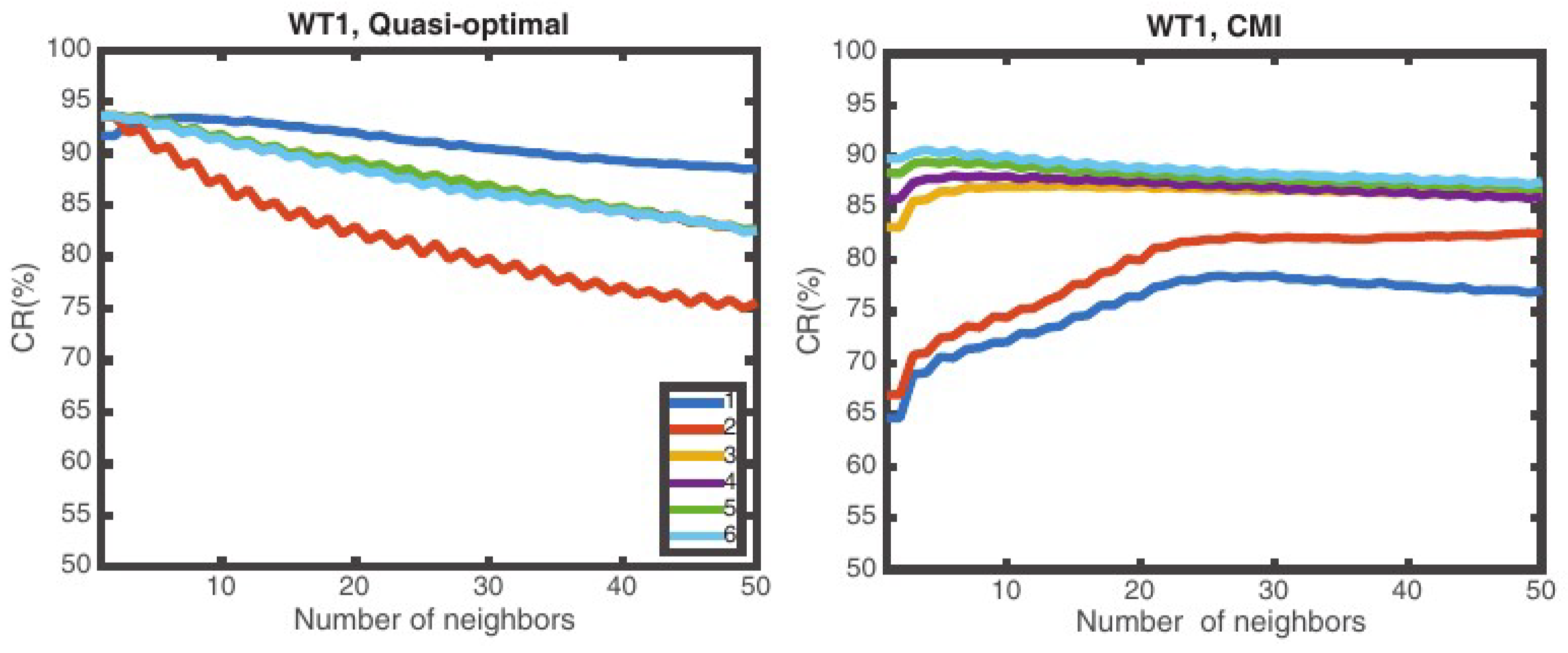
5.2. Effect of the Number of Neighbors Considered

To analyze the effect of the number of neighbors in the k-NN algorithm, experiments exploring all the cases for k = 1 to k = 50 in all the algorithms are performed, using the best combination of features for each case.

When analyzing the quasi-optimal case, k = 1 is the best option for all the WT. When using any of the automatic feature selection algorithms, if the number of features is small then the number of neighbors affects the CR and habitually k = 1 is not the best. Nevertheless, even increasing the number of neighbors, the obtained CR is lower that the QO case for the number of features analyzed. If the number of features increases, and therefore also the CR increases, k = 1 becomes again the best option and CR tends to the QO case. The advantage of increasing the neighbors is compensated by increasing the number of features. This effect can be observed in Figure 5: On the left column, the evolution of the CR as a function of k, for the quasi-optimal set of features (1 to 6) for WT1 and WT3, is presented. On the right column, the same WT but now using features obtained with the best feature selection algorithm among all the analyzed algorithms. Note that increasing the number of neighbors is only useful for the CMI algorithm when the number of features used is small (1 or 2), but does not help increase the CR when the number of features is larger. For the quasi-optimal feature selection algorithm, k = 1 is (almost) always the best option regardless of the number of features. Therefore, changing the number of neighbors has only impact when using 1 or 2 features in the CMI algorithm and degrades CR when the number of features is large or when the QO method is used.

6. Conclusions

In this paper, several methods for automatic feature selection for wind turbine failure prediction are explored and their performances are compared against the proposed quasi-optimal feature selection method detailed in Section 4.2. Experimental results using the 36 sensor variables listed in Table 2 show that CMI algorithm obtains good CR for all the wind turbine with up to six features and only one neighbour. Therefore, the speed of the system can be increased by using this algorithm instead of exhaustive search-based quasi-optimal strategy. The advantages are its low computational costs and fast speed calculations in order to find the best subset of features for wind turbine failure prediction. Although our study confirms that a selected set of three to six more discriminant variables are required to obtain the best prognosis performance, that selection is rather difficult to be represented. This is why sets of three selected variables, admitting a 3D Cartesian plot, becomes interesting. In this scenario, time evolution can be included generating plot animations. These dynamic representations provide powerful and intuitive insights about the behaviour of variables 21 days before failure occurs and becomes a useful tool to improve the models used for prognostic. In future works the dynamic representations of three features will be explored, allowing to visualize interactions between them, with the aim of simplifying and facilitating the management of wind farms.

References

1. European Commission. European Commission Guidance for the Design of Renewables Support Schemes; Official Journal of the European Union: Brussels, Belgium, 2013; p. 439. [Google Scholar]
2. The European parliament and the council of the European Union. Guidelines on State Aid for Environmental Protection and Energy 2014–2020; Official Journal of the European Union: Brussels, Belgium, 2014; pp. 1–55. [Google Scholar]
3. David Bailey, E.W. Practical SCADA for Industry; Elsevier: Amsterdam, The Netherlands, 2003. [Google Scholar]
4. IEC. International Standard IEC 61400-25-1; Technical Report; International Electrotechnical Commission: Geneva, Switzerland, 2006. [Google Scholar]
5. García Márquez, F.P.; Tobias, A.M.; Pérez, J.M.P.; Papaelias, M. Condition monitoring of wind turbines: Techniques and methods. Renew. Energy 2012, 46, 169–178. [Google Scholar] [CrossRef]
6. Romero, A.; Lage, Y.; Soua, S.; Wang, B.; Gan, T.-H. Vestas V90-3MW Wind Turbine Gearbox Health Assessment Using a Vibration-Based Condition Monitoring System. Shock Vib. 2016, 2016, 18. [Google Scholar] [CrossRef]
7. Weijtjens, W.; Devriendt, C. High frequent SCADA-based thrust load modeling of wind turbines. Wind Energy Sci. 2017. [Google Scholar] [CrossRef]
8. Wilkinson, M. Use of Higher Frequency SCADA Data for Turbine Performance Optimisation; Technical Report; DNV GL, EWEA: Brussels, Belgium, 2016. [Google Scholar]
9. Vestas R&D Department. General Specification VESTAS V90 3.0MW; Technical Report; Vestas Wind Systems: Ringkobing, Denmark, 2004. [Google Scholar]
10. Tyagi, P. The Case for an Industrial Big Data Platform; Technical Report; General Electric (GE): Boston, MA, USA, 2013. [Google Scholar]
11. Henry Louie, A.M. Lossless Compression of Wind Plant Data. IEEE Trans. Sustain. Energy 2012, 2012, 598–606. [Google Scholar] [CrossRef]
12. Vestas&IBM. Turning Climate into Capital with Big Data; Technical Report; International Business Machines Corporation (IBM): Armonk, NY, USA, 2011. [Google Scholar]
13. Shafiee, M.; Patriksson, M.; Strömberg, A.B.; Tjernberg, L.B. Optimal redundancy and maintenance strategy decisions for offshore wind power converters. Int. J. Reliab. Qual. Saf. Eng. 2015, 22, 1550015. [Google Scholar] [CrossRef]
14. Hameed, Z.; Hong, Y.; Cho, Y.; Ahn, S.; Song, C. Condition monitoring and fault detection of wind turbines and related algorithms: A review. Renew. Sustain. Energy Rev. 2009, 13, 1–39. [Google Scholar] [CrossRef]
15. Astolfi, D.; Castellani, F.; Scappaticci, L.; Terzi, L. Diagnosis of Wind Turbine Misalignment through SCADA Data. Diagnostyka 2017, 18, 17–24. [Google Scholar]
16. Astolfi, D.; Castellani, F.; Garinei, A.; Terzi, L. Data mining techniques for performance analysis of onshore wind farms. Appl. Energy 2015, 148, 220–233. [Google Scholar] [CrossRef]
17. Qiu, Y.; Feng, Y.; Tavner, P.; Richardson, P.; Erdos, G.; Chen, B. Wind turbine SCADA alarm analysis for improving reliability. Wind Energy 2012, 15, 951–966. [Google Scholar] [CrossRef]
18. Gray, C.S.; Watson, S.J. Physics of failure approach to wind turbine condition based maintenance. Wind Energy 2010, 13, 395–405. [Google Scholar] [CrossRef]
19. Bartolini, N.; Scappaticci, L.; Garinei, A.; Becchetti, M.; Terzi, L. Analysing wind turbine states and scada data for fault diagnosis. Int. J. Renew. Energy Res. 2017, 7, 323–329. [Google Scholar]
20. Garcia, M.C.; Sanz-Bobi, M.A.; del Pico, J. SIMAP: Intelligent System for Predictive Maintenance: Application to the health condition monitoring of a windturbine gearbox. Comput. Ind. 2006, 57, 552–568. [Google Scholar] [CrossRef]
21. Singh, S.; Bhatti, T.; Kothari, D. Wind power estimation using artificial neural network. J. Energy Eng. 2007, 133, 46–52. [Google Scholar] [CrossRef]
22. Zaher, A.; McArthur, S.; Infield, D.; Patel, Y. Online wind turbine fault detection through automated SCADA data analysis. Wind Energy 2009, 12, 574–593. [Google Scholar] [CrossRef]
23. Marvuglia, A.; Messineo, A. Monitoring of wind farms’ power curves using machine learning techniques. Appl. Energy 2012, 98, 574–583. [Google Scholar] [CrossRef]
24. Liu, H.; Tian, H.; Liang, X.; Li, Y. Wind speed forecasting approach using secondary decomposition algorithm and Elman neural networks. Appl. Energy 2015, 157, 183–194. [Google Scholar] [CrossRef]
25. Bangalore, P.; Tjernberg, L.B. Self evolving neural network based algorithm for fault prognosis in wind turbines: A case study. In Proceedings of the 2014 International Conference on Probabilistic Methods Applied to Power Systems (PMAPS), Durham, UK, 7–10 July 2014; pp. 1–6. [Google Scholar]
26. Cui, Y.; Bangalore, P.; Tjernberg, L.B. An Anomaly Detection Approach Based on Machine Learning and SCADA Data for Condition Monitoring of Wind Turbines. In Proceedings of the 2018 IEEE International Conference on Probabilistic Methods Applied to Power Systems (PMAPS), Boise, ID, USA, 24–28 June 2018; pp. 1–6. [Google Scholar]
27. Bangalore, P.; Tjernberg, L.B. An artificial neural network approach for early fault detection of gearbox bearings. IEEE Trans. Smart Grid 2015, 6, 980–987. [Google Scholar] [CrossRef]
28. Mazidi, P.; Bertling Tjernberg, L.; Sanz-Bobi, M.A. Performance Analysis and Anomaly Detection in Wind Turbines based on Neural Networks and Principal Component Analysis. In Proceedings of the 12th Workshop on Industrial Systems and Energy Technologies, Madrid, Spain, 23–24 September 2015. [Google Scholar]
29. Mazidi, P.; Tjernberg, L.B.; Bobi, M.A.S. Wind turbine prognostics and maintenance management based on a hybrid approach of neural networks and a proportional hazards model. Proc. Inst. Mech. Eng. Part O J. Risk Reliab. 2017, 231, 121–129. [Google Scholar] [CrossRef]
30. Mazidi, P. From Condition Monitoring to Maintenance Management in Electric Power System Generation with focus on Wind Turbines. Ph.D. Thesis, Universidad Pontificia Comillas, Madrid, Spain, 2018. [Google Scholar] [CrossRef]
31. Schlechtingen, M.; Santos, I.F.; Achiche, S. Wind turbine condition monitoring based on SCADA data using normal behavior models. Part 1: System description. Appl. Soft Comput. 2013, 13, 259–270. [Google Scholar] [CrossRef]
32. Astolfi, D.; Scappaticci, L.; Terzi, L. Fault diagnosis of wind turbine gearboxes through temperature and vibration data. Int. J. Renew. Energy Res. 2017, 7, 965–976. [Google Scholar]
33. Vidal, Y.; Pozo, F.; Tutivén, C. Wind turbine multi-fault detection and classification based on SCADA data. Energies 2018, 11, 3018. [Google Scholar] [CrossRef]
34. NREL. NWTC Information Portal (FAST). 2018. Available online: https://nwtc.nrel.gov/FAST (accessed on 10 January 2019).
35. Leahy, K.; Hu, R.L.; Konstantakopoulos, I.C.; Spanos, C.J.; Agogino, A.M.; O’Sullivan, D.T.J. Diagnosing and predicting wind turbine faults from SCADA data using support vector machines. Int. J. Progn. Health Manag. 2018, 9, 1–11. [Google Scholar] [CrossRef]
36. Kusiak, A.; Li, W. The prediction and diagnosis of wind turbine faults. Renew. Energy 2011, 36, 16–23. [Google Scholar] [CrossRef]
37. Leahy, K.; Gallagher, C.; O’Donovan, P.; Bruton, K.; O’Sullivan, D.T.J. A Robust Prescriptive Framework and Performance Metric for Diagnosing and Predicting Wind Turbine Faults Based on SCADA and Alarms Data with Case Study. Energies 2018, 11, 1738. [Google Scholar] [CrossRef]
38. Du, M.; Tjernberg, L.B.; Ma, S.; He, Q.; Cheng, L.; Guo, J. A SOM based Anomaly Detection Method for Wind Turbines Health Management through SCADA Data. Int. J. Progn. Health Manag. 2016, 7, 1–13. [Google Scholar]
39. Blanco-M, A.; Gibert, K.; Marti-Puig, P.; Cusidó, J.; Solé-Casals, J. Identifying Health Status of Wind Turbines by Using Self Organizing Maps and Interpretation-Oriented Post-Processing Tools. Energies 2018, 11, 723. [Google Scholar] [CrossRef]
40. Leahy, K.; Gallagher, C.; O’Donovan, P.; O’Sullivan, D.T.J. Cluster analysis of wind turbine alarms for characterising and classifying stoppages. IET Renew. Power Gener. 2018, 12, 1146–1154. [Google Scholar] [CrossRef]
41. Gonzalez, E.; Stephen, B.; Infield, D.; Melero, J. On the Use of High-Frequency SCADA Data for Improved Wind Turbine Performance Monitoring; Journal of Physics: Conference Series; IOP Publishing: Bristol, UK, 2017; Volume 926, p. 012009. [Google Scholar]
42. Zhao, Y.; Li, D.; Dong, A.; Kang, D.; Lv, Q.; Shang, L. Fault Prediction and Diagnosis of Wind Turbine Generators Using SCADA Data. Energies 2017, 10, 1210. [Google Scholar] [CrossRef]
43. Wang, K.S.; Sharma, V.S.; Zhang, Z.Y. SCADA data based condition monitoring of wind turbines. Adv. Manuf. 2014, 2, 61–69. [Google Scholar] [CrossRef] [Green Version]
44. Lewis, D.D. Feature selection and feature extraction for text categorization. In Proceedings of the Workshop on Speech and Natural Language; Association for Computational Linguistics: Stroudsburg, PA, USA, 1992; pp. 212–217. [Google Scholar]
45. Brown, G.; Pocock, A.; Zhao, M.J.; Luján, M. Conditional likelihood maximisation: a unifying framework for information theoretic feature selection. J. Mach. Learn. Res. 2012, 13, 27–66. [Google Scholar]
46. Battiti, R. Using mutual information for selecting features in supervised neural net learning. IEEE Trans. Neural Netw. 1994, 5, 537–550. [Google Scholar] [CrossRef] [PubMed] [Green Version]
47. Yang, H.H.; Moody, J.E. Data Visualization and Feature Selection: New Algorithms for Nongaussian Data; Advances in Neural Information Processing Systems (NIPS); MIT Press: Boston, MA, USA, 1999; Volume 99, pp. 687–693. [Google Scholar]
48. Meyer, P.E.; Bontempi, G. On the use of variable complementarity for feature selection in cancer classification. In Applications of Evolutionary Computing; Springer: Berlin, Germany, 2006; pp. 91–102. [Google Scholar]
49. Cheng, H.; Qin, Z.; Feng, C.; Wang, Y.; Li, F. Conditional mutual information-based feature selection analyzing for synergy and redundancy. ETRI J. 2011, 33, 210–218. [Google Scholar] [CrossRef]
50. Peng, H.; Long, F.; Ding, C. Feature selection based on mutual information criteria of max-dependency, max-relevance, and min-redundancy. IEEE Trans. Pattern Anal. Mach. Intell. 2005, 27, 1226–1238. [Google Scholar] [CrossRef] [PubMed] [Green Version]
51. Fleuret, F. Fast binary feature selection with conditional mutual information. J. Mach. Learn. Res. 2004, 5, 1531–1555. [Google Scholar]
52. Jakulin, A. Machine Learning Based on Attribute Interactions. Ph.D. Thesis, Fakulteta za racunalništvo in informatiko, Univerza v Ljubljani, Liubliana, Slovenia, June 2005. [Google Scholar]
53. Thomas, J.A.; Cover, T. Elements of Information Theory; Wiley: New York, NY, USA, 2006; Volume 2. [Google Scholar]
54. Cover, T.; Hart, P. Nearest neighbor pattern classification. IEEE Trans. Inf. Theory 1967, 13, 21–27. [Google Scholar] [CrossRef] [Green Version]
55. Domeniconi, C.; Yan, B. Nearest neighbor ensemble. In Proceedings of the 17th International Conference on Pattern Recognition, Cambridge, UK, 23–26 August 2004; Volume 1, pp. 228–231. [Google Scholar]
56. Zhou, Z.H.; Yu, Y. Adapt bagging to nearest neighbor classifiers. J. Comput. Sci. Technol. 2005, 20, 48–54. [Google Scholar] [CrossRef]
57. Hall, P.; Samworth, R.J. Properties of bagged nearest neighbour classifiers. J. R. Stat. Soc. Ser. B (Stat. Methodol.) 2005, 67, 363–379. [Google Scholar] [CrossRef] [Green Version]
58. Samworth, R.J. Optimal weighted nearest neighbour classifiers. Ann. Stat. 2012, 40, 2733–2763. [Google Scholar] [CrossRef]
Figure 1. Example of Wind Turbine sensors types. Adapted from TE connectivity (available via license: CC BY 4.0) http://www.te.com/.
Energies 12 00453 g001
Figure 2. Proposed exhaustive-search-based quasi-optimal algorithm.
Energies 12 00453 g002
Figure 3. General scheme of the experiments.
Energies 12 00453 g003
Figure 4. Evolution of the CR(%) against the number of features. (a) Quasi-optimal feature selection algorithm, all WT. (bf) Specific results for each WT and all the automatic feature selection algorithms analyzed. The dashed line in each panel corresponds to the quasi-optimal result for that specific WT.
Energies 12 00453 g004
Figure 5. Effect of the number of neighbors for WT1 and WT3. Each colored curve corresponds to a specific number of features, from 1 to 6. Only the QO and the CMI feature selection algorithms are reported here.
Energies 12 00453 g005aEnergies 12 00453 g005b