Computational Intelligence on Short-Term Load Forecasting: A Methodological Overview

Abstract

Electricity demand forecasting has been a real challenge for power system scheduling in different levels of energy sectors. Various computational intelligence techniques and methodologies have been employed in the electricity market for short-term load forecasting, although scant evidence is available about the feasibility of these methods considering the type of data and other potential factors. This work introduces several scientific, technical rationales behind short-term load forecasting methodologies based on works of previous researchers in the energy field. Fundamental benefits and drawbacks of these methods are discussed to represent the efficiency of each approach in various circumstances. Finally, a hybrid strategy is proposed.

1. Introduction

Short-Term load forecasting (STLF) is an integral part of the energy planning sector. Designing a time-ahead power market requires demand-scheduling for various energy divisions, namely, generation, transmission, and distribution. STLF helps power system operators with various decision-making in the power system, including supply planning, generation reserve, system security, dispatching scheduling, demand-side management, financial planning, and so forth. While STLF is particularly essential for the time-ahead power market operation, inaccurate demand forecasting will cost the utility a tremendous financial burden [1].

Traditionally, engineering approaches were employed to predict the future demand manually with the help of charts and tables. These traditional methods mainly considered weather impacts as well as calendar effects. Nowadays, these features are still determined for developing load models with novel methods [2].

With the advent of statistical software packages and artificial intelligence techniques, several outstanding pieces of research are devoted to statistical [3] and computational intelligence (CI) approaches [4] to model the future load. Some examples of statistical regression-based STLF approaches in the literature, including auto-regressive moving average (ARMA) [5,6], auto-regressive integrated moving average (ARIMA) [7], and seasonal ARIMA (SARMIA) [8]. Artificial neural network (ANN) [4], support vector machine (SVM) [9], fuzzy logic [10], etc., are considered prevailing CI-based forecasting techniques.

CI-based load models, regardless of underlying computational algorithms, can be further categorized into several methodological outlines. Correspondingly, it must be acknowledged that different forecasting techniques cannot be interpreted as different methodological approaches. A method is defined as a structured procedural solution designed for specific cases of forecasting practices; while a technique refers to a certain model that can be categorized with all other similar models in one technical category such as regression or neural network techniques. For example, Fan & Hyndman [11] and Mandal et al. [12] both applied ANN architecture to develop a 24-hour ahead load model whereas different methodological approaches were considered in each of these papers. In [11], a stepwise method, which locates the lowest error in the model, is applied for selecting the optimal subset of variables including the historical load and meteorological variables. However, in [12], only daily load profiles similar to day-ahead load recognized by a similarity index (similar day type and similar weather) are fed into the engine. The solution is not always narrowed down to the technique that the forecasters use. Instead, the strategy to implement those techniques is important as well.

Generally, both methods and techniques are important when it comes to accurate estimation. However, limited literature is available for STLF methodologies. Most surveys in the literature are devoted to the investigation of different STLF techniques [13,14,15,16]. For example, Mogharm et al. [14] investigated STLF techniques by classifying them into two categories of statistical approaches and CI-based techniques. Hippert et al. [13] reviewed ANN-based STLF. Although these surveys addressed most applicable STLF techniques, this still might be unclear for young researchers to understand the merits behind developing any specific load model.

This paper explains the main framework of state-of-the-art methodologies applied for the CI-based STLF via examples of several case studies. A comprehensive overview of technical and computational difficulties for STLF is presented as well as the proposed strategies by various researchers to unravel them. These strategies are categorized into four main groups based on their identical topologies. The robustness of each method to deal with different type of load data is identified.

The rest of the paper is organized as follows. Section 2 presents a general overview of four principal methodologies, followed by four subsections wherein details of each method are fully described. Section 3 discusses the main advantages and disadvantages of STLF methods. Moreover, in Section 3, advantages of hybrid methods are highlighted, and a hybrid method is proposed. Finally, the concluding remarks are drawn in the last section.

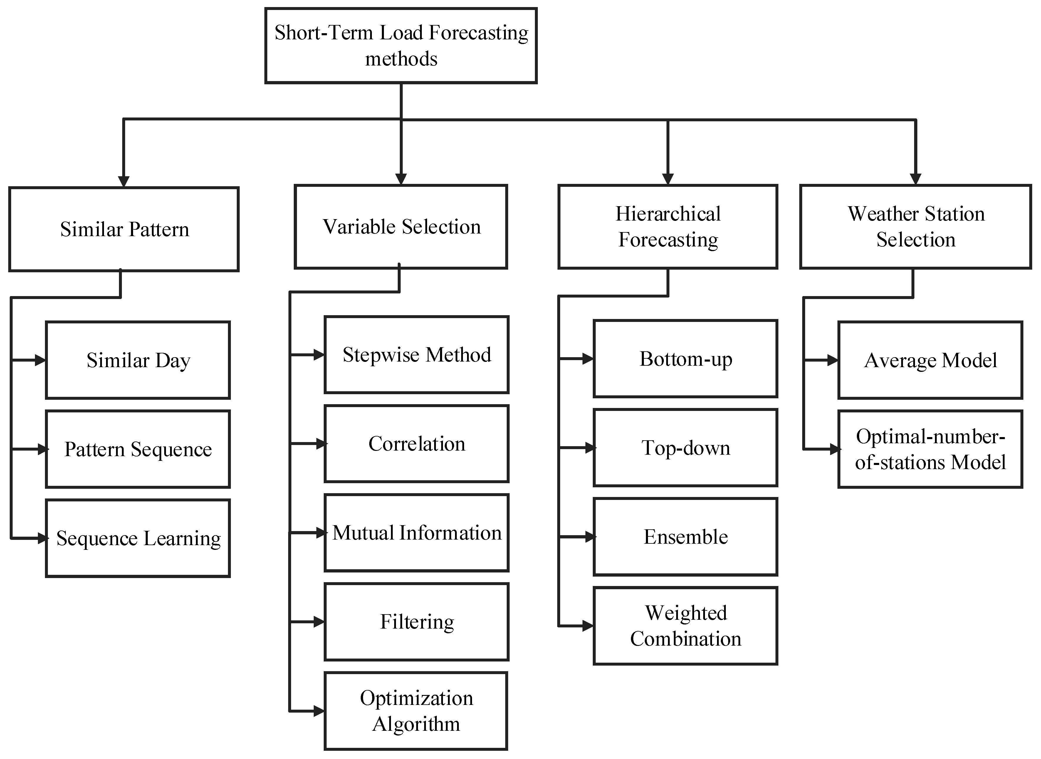
2. STLF Methodologies

Load forecasting can be conducted by various methodologies. The selection of a forecasting method relies on several factors including the relevance and availability of historical data, the forecast horizon, the level of accuracy for weather data, desired prediction accuracy, and so forth. Accordingly, selecting the proper load forecasting approach primarily depends on the time horizon of the prediction.

Different time horizons are adopted for load forecasting based on their specific applications in power system planning. For instance, the distribution and transmission planning are involved with STLF, while for longer durations, i.e., more than a year up to a few decades, the load prediction provides a decision platform for financial or power supply planning. Likewise, the required level of accuracy in these time horizons are not equal, as the decisions in the long-term are preliminary and may need significant changes in subsequent planning stages due to very uncertain input information while a short-term forecast provides information to the day-ahead market, which requires a high-level of accuracy. Moreover, different kinds of predictor variables are considered for each horizon of the forecast. For example, a long-term load forecasting takes into account population variations, economic development, industrial construction, and technology development whereas a short-term forecast mainly considers calendar variables, weather data, and customers’ behaviors [17].

Generally, both time categories of load forecasts are important for power system operation and development especially by the integration of distributed generators into the grid, which adds further intermittency and vulnerability in power provision. This study exclusively investigates the STLF approaches by reviewing original papers in this field. Even though some of the artificial intelligence (AI) techniques that are used for STLF might be also applicable for long-term load forecasting, on a methodological foundation, they are not comparable due to the aforementioned reasons.

Hong and Fan [2] identified four general categories of STLF methodologies, which can be applied to several techniques to solve the STLF problem. The four categories, i.e., similar day, variable selection, hierarchical forecasting, and weather station selection are specified based on different realizations of forecast problem. For example, similar-day method determines the load data as a sequence of various similar daily load profiles, while variable selection method presumes that the load data behaves like a series of variables either correlated or independent from each other. Hierarchical method, on the other hand, considers the data as an aggregated load, which is highly varying by changes in the load at lower levels of the hierarchy. Finally, weather station selection is a method, which determines the best-fitted weather data into the load model.

Hong and Fan outlined these general methodological approaches in a review [2], describing two or three examples of each, while an extensive literature of STLF has not been assessed accordingly. More investigation of the adopted STLF methodologies in the literature reveals that there are some novel approaches that could further be subcategorized into the four root categories. For example, the classic similar-day method, which distinguished the similarity between daily load profiles by assigning the day type index, was later developed as similar-pattern method, in which similar load profiles are extracted by using either a minimization algorithm or clustering techniques. Other novel approaches, such as pattern-sequence and sequence learning, are also recognized to be in the category of similar-pattern method, if their algorithms try to find or learn similar sequences of patterns within the dataset.

Moreover, the majority of STLF researchers chose the variable selection method, while different algorithms were employed for selecting prominent features of candidate variables. This research distinguished five state-of-the-art feature selection approaches for STLF. These approaches are specifically important to create the optimal subseries of data and leading to more accurate results.

Another category of STLF methodologies is assigned to hierarchical short-term load forecasting (HSTLF), which has been limitedly addressed in the literature. HSTLF methodology addresses forecasting at several levels of aggregate data. Although at each aggregate level, other methodologies, i.e., similar pattern and variable selection are used for individual predictions, the novelty of HSTLF is related to the applied combination method. Thus, four approaches are identified for HSTLF while each one proposes a different strategy. The classical top-down and bottom-up approaches are two common algorithms for hierarchical forecasting, with the latter aggregating the data and the former aggregating the forecast. Yet, recent approaches for hierarchical forecasting, i.e., weighted combination and ensemble model try to capture the model at each aggregate level individually and find the correlation between the individual models at different levels of the hierarchies. Despite limited literature, HSTLF lately received more attention by distribution and transmission operators for power system control and planning. It takes into account recent advances in communication infrastructures for remote measurement and automated metering, which enables operators with high granular data at user ends. Thus, the most recent challenges of HSTLF methodology is highlighted in this study to help young researchers find the competing research direction in this field.

By drawing attention towards HSTLF, a question might come to minds that by aggregating the data, what happens to other exogenous variables such as meteorological variables, as they cannot be aggregated. This challenge was raised for the first time by Hong and Pinson [18] and a competition was launched to address this question. Results of this competition are further discussed in this paper to draw a conclusion.

Figure 1 shows the tree diagram of these four forecasting methods. As can be seen, each method can be carried out via multiple strategies. For example, there are various approaches to predict a hierarchical structure including bottom-up, top-down, ensemble, and weighted combination. A full description of these four recognized categories of STLF methodologies is presented in the following subsections with examples of several case studies.

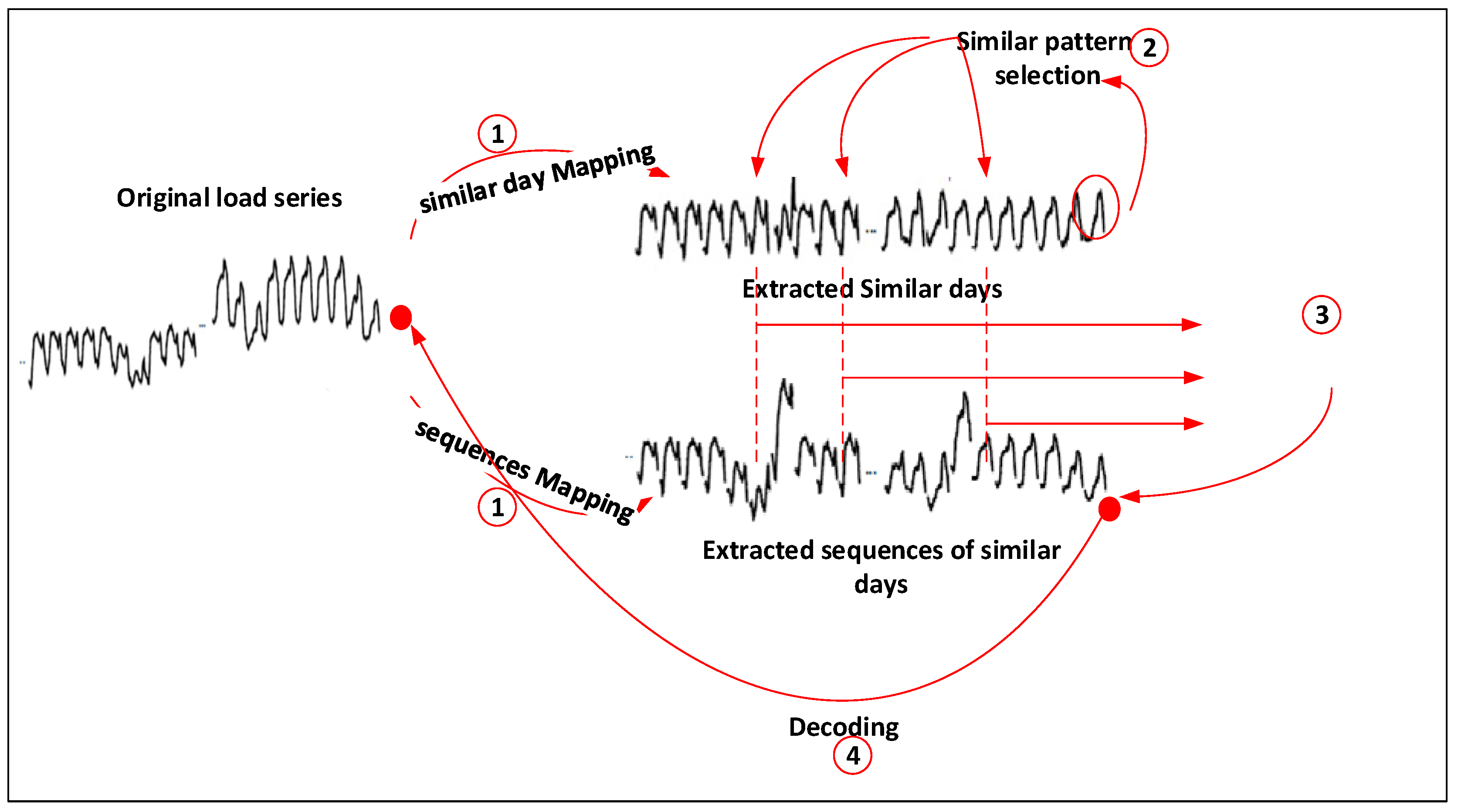
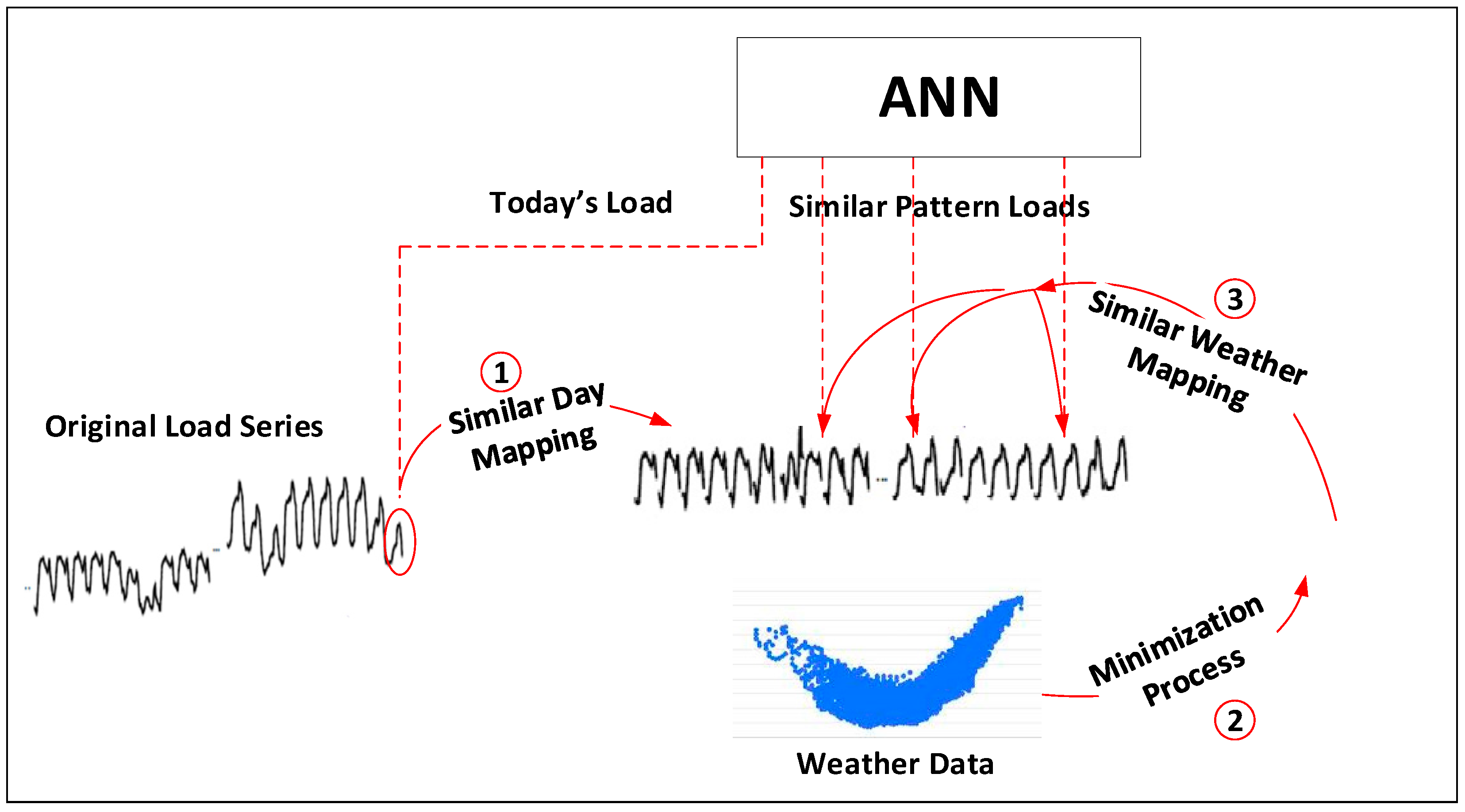
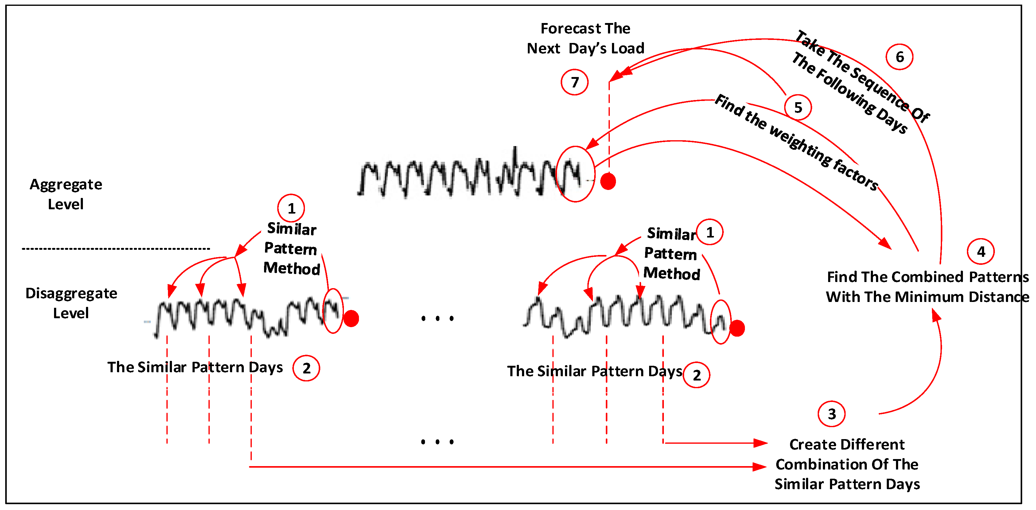
2.1. Similar-Pattern Method

Similarity-based methods are generalized forms of minimum distance approaches applied in machine learning and pattern recognition. These methods have also been used for STLF by finding similar demand patterns within the data set and predicting the future load using interpolation or weighting [19]. There are different strategies for finding similar load profiles; in the simplest case, it can be achieved by assigning a similarity index to the type-of-the-day in the calendar or meteorological factors. Similar patterns will then be achieved by searching between those days with similar indexes. Searching space is generally within a close neighborhood, although sometimes annual lagged data is also determined. For example, Dudek et al. [20] developed a similarity-based forecasting model by using the similarity between seasonal patterns of a load time series based on the calendar-lagged load data. The search space in [20] was limited to the nearest neighbor of the forecast day as well as the nearest neighbor of the same calendar day in the previous year. In fact, assigning the day-of-the-year index besides the weekday index is essential to avoid seasonal variations. A typical search space for similar-day method is illustrated in Figure 2.

Figure 3 illustrates the methodology applied by Dudek et al. [20]. In the first step, days similar to the forecast day with similar weekday and day-of-the-year indices are extracted from the load time series (first series). Thereupon, a sequence of days following these similar days (second series) is created. In the second step, days with similar patterns within the first series (similar-day series) are chosen by a selection strategy, and those followed by these newly selected days within the second series (sequence series). The outcome of the third step is a regression model of load data extracted from the sequence series. Eventually, the load of the next day in the original time series is forecasted by decoding the final model.

Besides the calendar index as the similarity indicator, other characteristics such as weather similarities can be considered as well. For instance, Ying Chen et al. [21] proposed a similar-day selection method based on the weather similarity of the forecast day. In their proposed method, which was designed to forecast the load in a short-term period (two working days excluding the weekend) by hourly resolution, the search for the similar days was limited to days with the same weekday and weather indices to the forecast day. Days with similar weather condition were selected based on a minimization process, while the meteorological condition was defined by wind chill, temperature, humidity, wind speed, and cloud cover variables. In addition, the same index was assigned for some of the weekdays with similar load pattern. It has also been shown that relying only on similar days’ data without establishing the initial status of tomorrow’s demand leads to an inaccurate forecast result. Thus, the 24-hour today’s load has been fed as an input to the forecasting engine. Figure 4 illustrates the schematic diagram of similar-day method developed in [21].

As already mentioned, the selection of similar load profiles between days with similar indexes (weekday, the day-of-the-year and weather indexes) can be made by a distance minimization technique. Some works in the literature applied Euclidean norm to measure the match level between similar days [12,21,22]. As listed in

Table 1. Distance minimization technique for similarity measurement.

Paper	Method	Formulae	Parameters
[21]	Euclidean distance minimization	$\underset{i}{\min }{\sum }_{t=1}^{24}\left(w{\left(t\right)}^f-w{\left(t\right)}^i\right), i\in \theta$ (1)	θ: historical days f: forecast day i: historical day in θ $w$: weather factor under consideration
[12,22]	Weighted Euclidean distance minimization	$\underset{t}{\min }\sqrt{w_1{\left(\Delta L_t\right)}^2+w_2{\left(\Delta L_s\right)}^2+w_3{\left(\Delta T_t\right)}^2}$ (2)	$\Delta L_t$: deviation of load of forecast day and historical day $\Delta L_s$: deviation of slope between load on forecast day and load of historical day $\Delta T_t$: deviation of temperature between forecast day and historical day $w_n$: Weight factor

, Chen et al. [21] used the Euclidean norm to evaluate the weather similarity between the forecast day and previous days. Senjyu et al. [22] also applied a weighted Euclidian to investigate the similarity of load patterns using load deviations between forecast day and historical days, weather deviation, and the slope of load deviations. The assigned weights (w) in Equation (2) is determined based on a regression model using the trend of load and temperature.

Dynamic time warping (DTW) is another method to measure the similarity for those time series with similar values not exactly at the same time point. Using DTW method might end up finding several similar patterns of load profiles within the dataset. Teeraratkul et al. [23] indicated that by using DTW method, the number of groups for similar profiles reduced by 50%.

More recently, clustering algorithms are used to find similar sequence of load patterns within the dataset [24,25]. These clustering techniques are used to group data into a specific number of categories of daily load patterns, which were termed pattern-sequence-based STLF method. Under this method, a label indexes the load for each day in the dataset. Consequently, a sequence of labels is created in the dataset. Alvarez et al. [26] applied K-means clustering technique to create different clusters of load patterns and extracted a sequence of labels from the dataset as a pattern to search and predict the next day’s load. A schematic diagram of pattern-sequence-based forecasting method is depicted in Figure 5. According to Figure 5, all weekdays in a dataset are labeled by using a clustering method. To predict the next day’s load, a window of a sequence of labels before the forecast day is selected. By using this window, similar sequence of labels is searched within the dataset. Eventually, the load of the target day can be predicted by averaging the next day’s load of the discovered sequences.

The prevalence of smart meters in a smart grid facilitated market planners with fine-grained data in hourly and sub-hourly resolution. Load profiles at the customer-end provide sophisticated information about the type of customers and their consumption behaviors. Quilumba et al. [27] used a clustering technique to group smart meter customers according to their similar energy pattern consumption. Temperature information was interpolated between neighbor values to become as granular as the smart data.

Clustering methods can distinguish similar sequences within a dataset as discussed earlier; however, they cannot differentiate among the main features of these patterns. More recently, adding memory to the structure of learning engines such as recurrent neural network and deep learning, outweighed this drawback.

Liu et al. [28] considered sequence learning approach for developing a load model by using recurrent neural network structure (RNN). Kong et al. [29] recommended that long short-term memory of RNN was a powerful engine to learn the look back sequences due to its memory cells, remember important features, and forget gates to reset the cells for redundant features. Shi et al. [30] applied deep RNN to map the sequence of input data into the corresponding output sequence. Zheng et al. [31] proposed a hybrid method, by applying a clustering technique to capture similar days within a dataset, and then used the sequence-to-sequence structure of the long short-term memory structure to adjust the length of the input and output sequences. A sequence-to-sequence structure was primarily designed to map sequences with different length [32,33]. Marino et al. [33] suggested that the main advantage of the sequence-to-sequence structure was related to its ability to predict an arbitrary number of future time steps having an arbitrary length of an input sequence. Satish et al. [34] investigated the optimum learning sequence for the training stage. Results indicated that the number of patterns in a sequence affected the accuracy of the model.

Table 2. Published articles employing similar-pattern method.

Method	Publications	Technique
Similar-Pattern Method
	[12,20,21,22,23,35,36]	similar day
	[24,25,26,27,37,38,39,40,41]	pattern-sequence
	[28,29,30,31,32,33,34]	sequence learning

lists some highly cited publications in which similar-pattern method was applied for load prediction. These publications are categorized based on three common techniques, namely, “similar-day”, “pattern-sequence”, and “sequence learning”.

In general, pattern similarity method is an efficient approach to capture repeated patterns of the load series in the short term. The overall pattern of a system is rarely changing in the short term; however, in longer periods, some significant deviations might lessen the similarity of future load to past load.

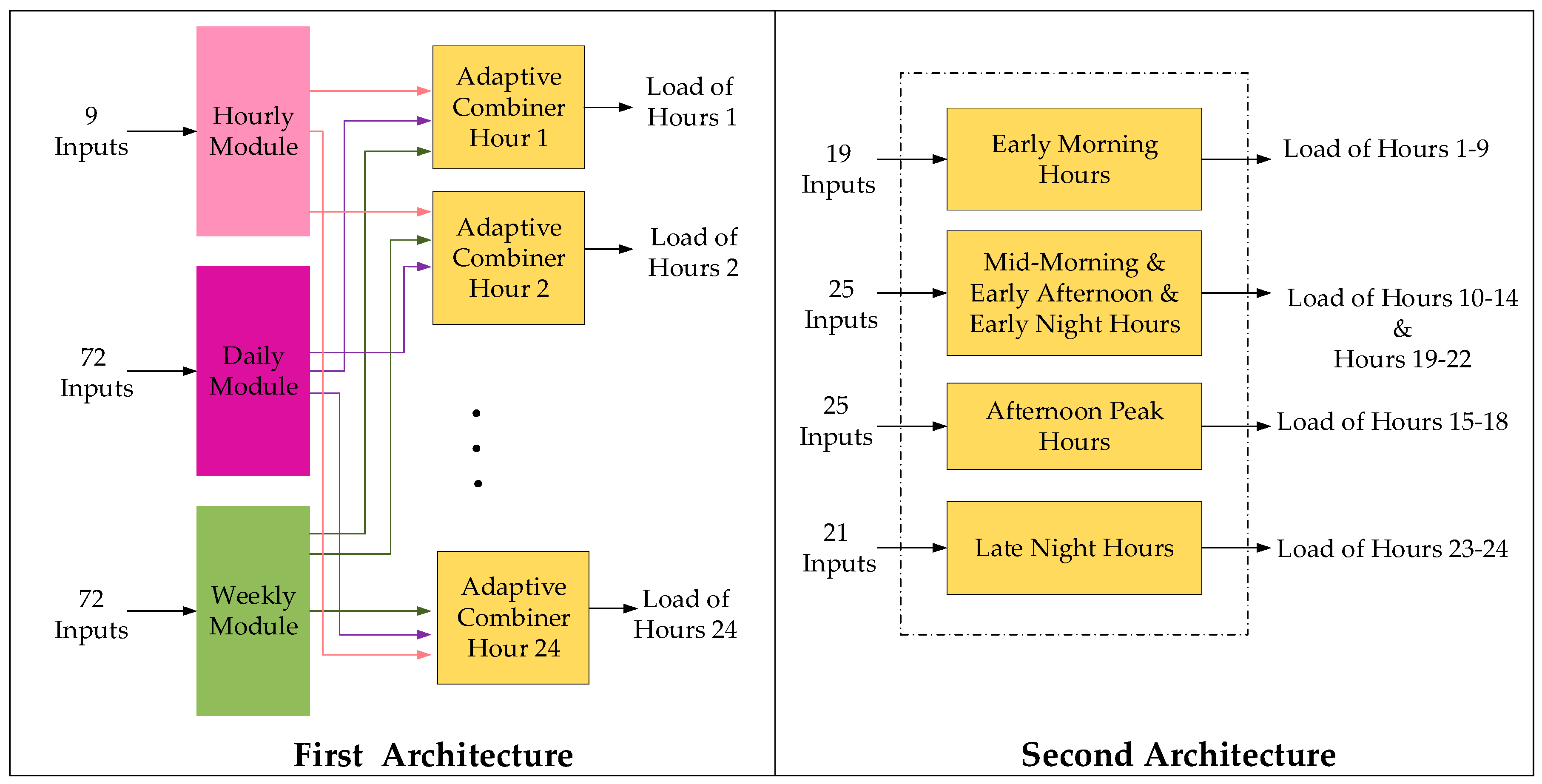
2.2. Variable Selection Method

Variable selection is the process of selecting the most influential variables or features (predictor variables) within the dataset while they can adequately capture the relationship between the available data and the output. Despite time series forecasting relies only on past data, variable selection method determines external variables besides historical load in order to embed into the model [42]. Some of these external variables, which are termed explanatory variables to explain the reason of load fluctuations, are calendar variables (time of the day, day of the week, month of the year, and day of the year etc.), meteorological variables (temperature, humidity, cloud cover, wind chill, solar radiation etc.) and so forth [43].

Several studies also considered the lagged load data into their model [44,45]. The lagged variables determine the recency effect by incorporating alteration of demand level throughout load time series into the model. For example, Ceperic et al. [44] proposed a feature selection algorithm to select the optimum number of lagged loads in order to embed the sequential correlation of load variables into the model. Another example is the work of Fan and Hyndman [11], which considered the following variables as candidate predictors: the lagged load demand for each of the preceding 12 hours, lagged values for the same hours of the two previous days, maximum and minimum load values in the past 24 hours, and the average load in the preceding week. Consequently, a selection algorithm was applied to choose between potential variables and create a subset of optimal predictor variables.

Besides the lagged demand, some studies embedded lagged temperatures as input variables. The electricity demand is remarkably impacted by the recent temperature as well as the current temperature. That is why in the forecasting model developed by Fan and Hyndman [11], besides the lagged demand, the current and 12-hour lagged temperature for the preceding day and the former two days were involved in the model. However, the main concern about weather variables was its level of validation, which depends partly on the weather station selection. It is discussed more in Section 2.4.

By nominating multiple input variables and considering a large amount of available data for every variable, the predictor engine might not be able to converge to an accurate predictive model. Therefore, an effective subset of the data with the optimal number of predictor variables will help the forecast accuracy [46]. An efficient predictor variable is highly explanatory and independent of other variables. The aim is to select the optimal subset of predictor variables with fewer numbers, which suitably describes the characteristics of the output variable. Optimal input subset favors model accuracy as well as cost efficiency and model interpretability [47].

In the literature, researchers employed different methods and techniques to select explanatory variables optimally.

One of the methods used for variable selection is the stepwise refinement which is a step by step approach for input selection. In this method, the primary model is a full model consisting of all measured variables. Hence, based on the predictive capability of individual variables, redundant terms from the model are omitted. The retained variables consequently lead to the best model. One example is the work of Fan and Hyndman [11], who carried out a step by step variable selection method to extract the best-suited model. The nominated inputs were the calendar variables, actual demand and lagged demand (from the National Electricity Market of Australia-NEM), and forecasted temperature data from more than one site in the target area. Assuming the selection of temperature differentials, in the first step, the temperature differentials form the same period of the last six days were dropped one at a time, and the one leading to the lowest error was selected. Consequently, in the next step, the temperature variable was frozen to only the selected day from the previous step, and temperatures of the last six hours were considered for the trial. This procedure was continued until the final group of variables was selected.

Nedellec et al. [48] followed the same strategy of stepwise refinement for variable selection as well, but in a three-step procedure while the variables in each stage were selected based on the scale of forecast. In a long-term module, monthly load and temperature time series for every region and weather station were selected to extract long-term trend and low-frequency effects. The residual of the first stage with no seasonality and weather effects were considered for a medium-term estimation. Variables such as a type-of-the-day, type-of-the-year, de-trended electrical load, real temperature, and lagged temperature were predictor variables in this medium-term model. In a short-term stage, more localized factors, which remained from previous stages, were captured by selecting variables such as year, month, day, hour, time-of-the-year, and day type as well as real and smoothed weather variables. This stepwise algorithm is illustrated in Figure 6 for better understanding. As can be seen, the final forecasted load is an additive model of three components.

Xiao et al. [49] also developed an ensemble load model by applying a group of STLF techniques to capture the trend of the load series. Consequently, the highly nonlinear characteristics of the residual subseries were modeled by using various data handling techniques.

Moreover, there are other approaches to identify the maximum relevance between different variables. Correlation-based methods use a heuristic algorithm to find a subset of variables, which are highly correlated with the output but are not correlated with each other [50]. Chen et al. [9] used correlation method to measure the dependency of the peak demand to temperature. Kouhi et al. [51] developed a correlation-based feature selection method to reduce chaotic structure of load time series and selected highly relevant variables within this reconstructed space. Amjady et al. [3] used a correlation approach to create a subseries of load data to develop a hybrid forecast model.

Mutual information (MI) is an information theoretic-based approach to measure the interdependency between two random variables. If MI is zero, two variables are independent and contain no mutual information about each other. Higher MI values indicate higher relevance with more information about the target feature [52]. Wang et al. [53] used MI method to obtain initial weights of the developed ANN-based load forecast model. Elattar et al. [54] reconstructed a load time series by embedding dimension and time delay computed by MI approach. Young-Min Wi et al. [55] adopted MI method to evaluate mutual information between dominant weather features and loads at different seasons.

Moreover, filtering methods can be applied to data to find the correlation among variables independent of any learning machine. Filter-based feature selection algorithms use general characteristics of the training data, i.e., statistical dependencies to select highly ranked features by applying a threshold for the number of features [56]. Reis et al. [57] applied wavelet filter to reconstruct a subseries of data after selecting input variables by using autocorrelation function. Amjady et al. [58] proposed a hybrid load prediction algorithm, in which a filter-based technique was selected for a minimum subset of inputs. Zhongyi Hu et al. [59] proposed a hybrid filter method for feature selection procedure.

More recently, developing bio-inspired optimization tools as well as evolutionary optimization algorithms led to improvement of CI-based feature selection techniques for STLF. Some examples of developed optimization algorithms for feature selection in the literature include ant colony [60], particle swarm [61,62], differential evolution [63], hybrid genetic and a colony [64] and so forth.

Some of the highly cited publications for STLF, which are categorized based on the applied feature selection techniques, are listed in

Table 3. List of publications employing different feature selection techniques.

Publication	Technique
[11,48,49]	Stepwise
[57,58]	Filter
[3,9,47,51,65,66]	Correlation
[47,53,54,55,67]	Mutual Information
[60,61,62,63,64,68,69]	Optimization Algorithms

.

Selecting proper variables is sometimes time-dependent, while variables have significant impacts on load behavior of several hours and subtle effects on loads of other hours during a 24-hour period. Thus, a suitable architecture for a forecasting engine can provide a simpler model to decrease the number of redundant data [70]. A general idea is that instead of creating one subseries of data, different subsets of variables can be created for each category of time, while data in each category is affected by the same variables. For example, Khotanzad et al. [71] proposed two different parallel architectures for load forecasting. The first design, as illustrated in Figure 7, was a three-module structure to model hourly, daily, and weekly trends. In their developed architecture for prediction of the hourly load of the next day, each of three modules would be trained by 24 ANN engines. Each of them represented an hour of a day. The second architecture divides 24 hours into four categories, i.e., 1–9, 10–14 and 19–22, 15–18, and 23–24 while different input variables are determined for each group of hourly loads, as depicted in Figure 7.

Some other papers in the literature also applied the so-called parallel architecture for 24-hour-ahead load forecasting [44,72]. The reasons for using this design are smaller number of training data for each module with omitted parameters for each hour of the day, and a simpler model for each hour of the day, compared to a general model for all 24 hours.

In overall, developing an explanatory model via variable selection method is appropriate when forecasters have fundamental knowledge about the system. To forecast the variable of interest, one needs to identify different exogenous variables. Generally, there are no rules implied for the selection of input variables. The forecaster’s experiences in analyzing the type of data from a specific market as well as a preliminary testing might help to select a proper group of variables. Thus, professional judgment is undoubtedly part of the process.

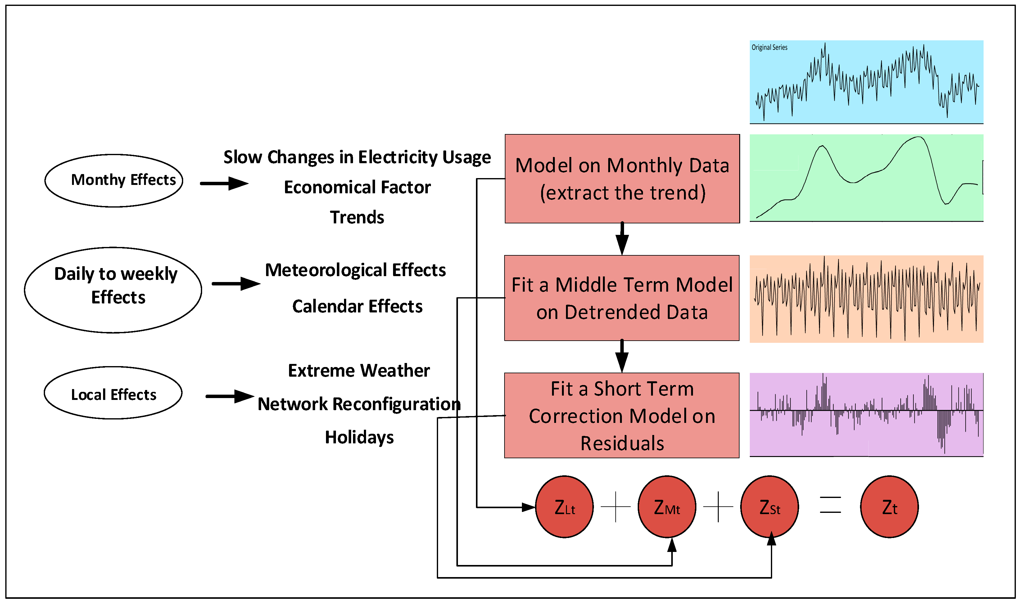
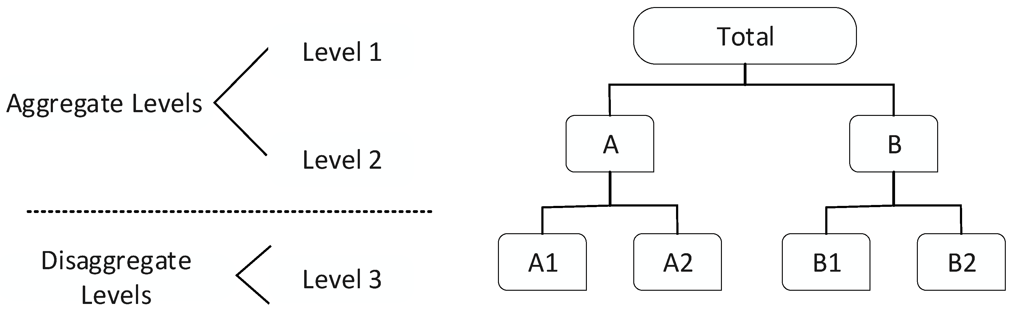
2.3. Hierarchical Forecasting

Previous methods presume load data as single time series, while these time series can be inherently disaggregated by different attributes of interest [42]. Load time series naturally are organized based on different hierarchies such as geographic, temporal, circuit connection, and revenue. Figure 8 depicts a typical hierarchical structure of a time series divided into aggregate and disaggregate levels.

An example of hierarchical load structure can be found in a study conducted by Zhang et al. [73]. The load data was recorded consumption of three hundred smart meter customers of a subsection in Australian utility within three years. The customers were clustered into 30 nodes according to their postcodes. These 30 nodes were grouped into three nodes. Besides, these three nodes were summed up at the final level to an aggregated time series. In the distribution level, however, the hierarchical levels were specified as load of substations, feeders, transformers and, customers [74].

Recently, there has been a prevailing attention to HSTLF due to market considerations for decision-making in different levels of the power system including independent system operator, distribution operator, and customer-end. Utilities require load forecasting at low voltage levels to effectively perform distribution operation such as circuit switching and load control. An accurate load forecasting at low level could even increase the prediction accuracy at independent system operator level [75]. In fact, the independent system operator in the upper level in a power system covered a large geographical area, with extensive load diversities throughout the area. Hence, a single model was not able to guarantee the prediction accuracy.

The state-of-the-art HSTLF methods to address hierarchical load structure are sub-grouped into bottom-up and top-down approaches [27,76]. The bottom-up approach aggregates forecasts from low level to aggregated level, while the top-down method aggregates historical load prior to forecasting. The former approach does not miss out any information due to the aggregation, although high volatility of bottom level is challenging for prediction [77]. The top-down method, on the other hand, is simpler for less noisiness due to the aggregation. However, some features of the individual series are lost [42]. For instance, Quilumba et al. [27] used the bottom-up approach for forecasting load of the customers disaggregated by similar consumption patterns.

Some of the advantages and disadvantages of bottom-up and top-down approaches were highlighted by Hyndman et al. [78] who referenced early works in the literature. Generally, the bottom-up approach was robust when the data in bottom level was reliable without missing information. Otherwise, the forecast at a low level was error-prone and the top-down approach resulted in a more accurate forecast. Overall, the superiority of a method over another was not uniform.

HSTLF can also be conducted at all levels of hierarchies individually, which is termed “base forecast”. However, the challenge here is that the prediction at aggregated level might not be consistent with the summed base forecasts [79].

Zhang et al. [73] proposed a solution to optimally adjust base forecast at each node in order to be consistent across the aggregation structure. This goal was accomplished by minimizing the redundancy between the forecast at the aggregated level and the sum of the base forecasts, by using quadratic programming in a post-processing scheme. The method was tested on two electricity networks; one bulk system of a large area with several dispatch zones at the bottom level, and the other was a distribution network covering a small area with hundreds of individual customers. Results indicate that for more than 85% of nodes in the bulk network, the proposed method was more accurate. For distribution network with more volatile load, the improvement was more obvious, especially at upper aggregated level where the error was significantly decreased. Nose-Filho et al. [80] also developed a load model for a sub-distribution system in New Zealand by finding participation factors between local forecasts and global forecast.

Another example is the study by Fan et al. [81], who proposed a strategy to forecast load of sub-regions within a large geographical area independently by finding the optimal region partition in the combination procedure. It was reported in [81] that the weather condition was a dominant factor for load variations and therefore, in a large geographical region, the extreme weather condition throughout the area caused high load diversity. Another factor that rendered regional load profiles vastly different was identified in [81] as non-coincident load peaks.

Sun et al. [74] proposed a strategy to predict loads of different nodes in a power distribution system by a top-down approach. Firstly, loads of parent nodes were forecasted. Subsequently, by finding the similarity between the parent node (aggregated level) and its child nodes (correspondent disaggregated levels), two classes of regular and irregular nodes were identified. Thus, for regular nodes, the load is a fraction of the origin load computed by a distribution factor. For those irregular loads, which did not follow leading characteristics of the parent node, individual models were forecasted. The similarity between nodes was identified by using distance minimization method for both weather parameter and historical load.

More recently, with the dominance of smart meters, fine-grained data at sub-levels revealed more information at the aggregate level. Wang et al. [82] used granular smart meter data to construct a forecast model at an aggregated level. In their proposed model, data was clustered into different groups of loads with similar patterns, and the aggregated forecast was obtained by adding the forecast of individual clusters. However, instead of the bottom-up strategy, a weight was assigned to each model while varying the number of clusters. The final forecast was an optimally weighted combination of these individual forecasts. Their proposed method was implemented on a data set consisting of 5237 residential consumers’ information with half-hourly resolution for 75-week duration. It was shown that results of the direct aggregated load were more accurate than the clustering strategy although their proposed methodology outweighed the conventional bottom-up method. Besides this data set, the method was tested on 155 substations’ load data for a 103-week duration. In contrast to the first data set, the outcomes of the forecast on the second dataset indicated that the bottom-up model was more accurate than other individual clustering models. It was concluded that this contrast was due to regularity in substation load in comparison to residential load profiles.

Table 4. Combination methods for base forecasts.

Combination Method	Formulae	Parameters
Linear Programming	$w=\arg \underset{\mathrm{w}}{\min }{\displaystyle {\displaystyle \sum }_{t=1}^T}\frac{1}{T}\frac{\left|\widehat{Y}-\tilde{Y}\right|}{\widehat{Y}}$ $\tilde{Y}={\displaystyle {\displaystyle \sum }_{n=1}^N}{w}_n{\tilde{Y}}_n$	$\widehat{Y}$: base forecast $\tilde{Y}$: adjusted forecast $w$: weight factor
Quadratic Programming	$\underset{\tilde{Y}}{\min }\frac{1}{2}{(\widehat{Y}-\tilde{Y})}^T{\Sigma }^{-1}(\widehat{Y}-\tilde{Y})$ $\tilde{Y}={\left[{\tilde{a}}^T,{\tilde{b}}^T\right]}^T$ $\tilde{a}=p\tilde{b}$	$\widehat{Y}$: base forecast $\tilde{Y}$: adjusted forecast $\tilde{a}$: load of the aggregated level $\tilde{b}$: Load of the disaggregated level $p$: participation factor

illustrates two combination methods, which were applied to sum up base forecasts for maintaining its coherence with the aggregated forecast. Both of these methods minimized the error between the summed up base forecasts and aggregated forecast, either by linear [82] or quadratic [73] programming. Other combination methods were discussed in [83] with further theoretical explanations. This is suggested that new HSTLF methods might be expressed by selecting an appropriate combination algorithm.

Different levels of a hierarchical structure interacted with each other in a complicated fashion, whereas a change in one series at one level could sequentially change the series at the same level as well as other levels of a hierarchy. Sun et al. [74] considered the change that switching operation might cause on the load trend by adjusting the forecast whenever a switching was detected. Abnormal changes in the demand were identified by measuring the mean and standard deviation of the load by using statistical process control. The load participation factor was then computed based on the new data. Comparably, deviations in the meteorological conditions in a large geographical area caused base forecasts to vary, leading to changes in the aggregated load accordingly. However, meteorological information might not be available at every sub-level. There were usually several meteorological services available at a geographical area for providing weather forecast information. Hong et al. [18] recommended that, in a hierarchical structure with various nodes to be forecasted, the best-related weather information could not be selected manually for each node. Weather station selection method was one of the main objectives in the Global Energy Forecasting Competition 2012 (GEFC) [84]. More about this is discussed in the next section.

2.4. Weather Station Selection

In a large electricity market covering an expanded area, a single forecasting model cannot capture the load pattern. HSTLF method, which is discussed in the previous section, ensures a more satisfactory forecast across different levels of hierarchy. However, in HSTLF method that disaggregates the load based on geographical divisions or zonal hierarchies, meteorological hierarchies that are definitely a dominant factor in load diversity cannot be easily captured. The challenge is to assign the most related weather station information to each zone or area in the hierarchy.

Fan et al. [81] proposed a combination method to select the best adapted individual weather forecast between multiple forecasts provided by different meteorological services. Several papers in the literature [85,86] used the average data from multiple services for its simple and effective result compared to other weighted averaging methods.

In Hong & Pinson’s planned competition (GEFC competition) [18], weather station selection was one of the addressed issues. Data provided in the competition was the hourly load history of 20 zones in the U.S. along with weather data gathered from 11 weather stations, without specifying locations of weather stations.

Among the winning teams, Charlton et al. [87] built 11 energy models for each zone based on the weather data of 11 weather stations provided in the competition. The best-fitted weather station for each zone was not a single station, rather, it was a linear combination of up to five best-fitting weather stations for each group. Lloyd [88] also developed a forecast model based on data from all weather stations and used a Bayesian model averaging to integrate these models into one final average model. Moreover, in the proposed model by Nedellec et al. [48], one station was selected for each zone, considering that other combination strategies led to unsatisfactory outcomes. Taieb et al. [89] selected the best-fitted station for each zone by testing the temperature data from previous week for each zone. The demand was modeled by using average temperature data of three best weather sites. Hong et al. [18], on the other hand, proposed a method for weather station selection that, instead of assigning the same number of weather station to all nodes at the same level of hierarchy (as it was the common strategy in the GEFC competition), different numbers of weather stations were selected for individual load zones. Yet, the result was not always superior to other alternatives.

3. Method Evaluation and Future Work

A comprehensive explanation of STLF methodologies is provided in the previous sections. Generally, the logic behind every specific method helps the forecaster to choose the best-fitted method based on their application. For example, similar-pattern method mainly relies on historical values, whereas variable selection method incorporates information about explanatory variables. Therefore, the forecaster might consider similar-pattern method in cases where the system might not be comprehensive enough, or if it is explanatory, it is extremely difficult to extract the main features that govern the demand behavior. In this situation, there are always some variations in the load that cannot be captured by explanatory variables. In similar-pattern strategy, on the other hand, the focus is on what is going to happen rather than why it happens. Still, when there is a correlation between exogenous variables and load data, explanatory model, i.e., variable selection method is an appropriate approach.

Some of the main advantages and disadvantages of these four methods are listed in

Table 5. Advantages and disadvantages of STLF methodologies.

Method	Advantages	Disadvantages
Similar-Pattern Method	Adapt to exceptional circumstances and random events No previous knowledge about the system is needed	The horizon of forecast is limited up to a couple of days ahead Limited search space Not explanatory
Variable Selection Method	Embedding exterior variables into the model Increase prediction accuracy by reducing overfitting and addressing the curse of dimensionality Simpler prediction (smaller number of predictors or smaller size of input space) Improves the understanding of the prediction model	The load data might not be comprehensive (difficult to measure the relationship that govern the load’s behavior) Difficulty in identifying exogenous variables Huge number of variables Redundancy It is unrealistic to find a set of input variables with zero correlation to each other
Hierarchical Method	Help the power system operators to perform the load control and circuit switching at different levels of the hierarchies Enhancing the model accuracy by using the information at the lower levels	Lack of coherency across the aggregated structure Loss of information due to aggregation in the top levels The high irregular data at the bottom levels of the hierarchies
Weather Station Selection	Find the best-fitted weather data for each level of the hierarchy	Uncertainty about optimal number of stations for each hierarchy

. For example, in variable selection method, despite efforts to find independent variables in the dataset by using feature selection algorithms, the selected variables might still be partly correlated with each other. This matter is expressed as one of the drawbacks in Table 5. Similar-pattern method, on the other hand, presumes that the past values of a variable are important in predicting the future, although the algorithms can only look back for a few steps for a limited sequence of data.

Despite the unique characteristics of these four categories of STLF methodologies, they were not independent of each other and there might be some overlap between them. For example, in similar-pattern method, the similarity of exogenous variables such as temperature or humidity were used to find similar patterns [21]. Consequently, selection of highly correlated exogenous variables is essential for detecting similar load patterns within a dataset.

Sometimes the selection of exogenous variables in variable selection method was conducted by using similarity method. For example, Fujimoto et al. [90] applied the minimum distance technique to find the relationship between exogenous variables and residential demands of multiple houses.

Another example was HSTLF method, as already discussed in Section 2, wherein either variable selection method or similar-pattern method was applied to forecast the load at each level of aggregation. Similarly, for weather station selection, a forecaster addressed a subset of exogenous variables, i.e., meteorological variables.

Hyndman et al. [78] discussed that taking advantage of the prominent features of different methods and combining them in a hybrid scheme was what we needed to do now. Some examples of this combination were available in the literature. For example, Quilumba et al. [27] applied similar-pattern method in one step to group smart meter load profiles into an optimal number of groups and then feature selection method in the next step to forecast the aggregated load at each group of data.

In the proposed load model by Wang et al. [82], a three-stage combined model was applied. The hierarchical structure of the load series was extracted by applying hierarchical clustering technique based on similar consumption behavior of customers. Different load models were developed at each subgroup of data by using variable selection method. Eventually, the final model was undertaken by adding a weight factor to individual models to be coherent across the aggregate level.

Another example of the hybrid methodology could be found in the work of Zheng et al. [31], in which feature selection method was used to help find similar days’ clusters. Each cluster was shaped based on feature values of the data, whereas a weighted parameter was assigned to each feature.

In this paper, a hybrid method is represented based on some of the main features of methods reviewed in the previous sections. The schematic diagram of the method is illustrated in Figure 9. As can be seen, this method is proposed to find base forecasts at each level of the hierarchical structure by applying similar-pattern method, and then by using a strategy to keep the coherency between the loads at different levels. The strategy is performed in seven steps as shown in Figure 9. In the first step, the patterns similar to today’s load profile are extracted from each load series at the disaggregate level. Considering that n number of similar patterns are obtained for each subseries, and by assuming that there is N number of subseries at the disaggregate level, n^N number of aggregated profiles is created. Between these aggregated profiles, the one with the minimum distance from today’s profile at the aggregated level is selected. Subsequently, in the next step, the combined profile will be matched to the real aggregated profile by finding the weighting factor. Eventually, to forecast the next day’s load at the aggregated level, load profiles of sequential days (days after similar-pattern days), which are selected in the optimal combination, will be summed up by using the weighting factor of step 5. This method finds similar patterns in the disaggregated level, but measures the similarity distance again at the aggregated level.

The novelty of the proposed method over the aforementioned hybrid method is that it neither aggregates the data from bottom levels nor aggregates low-level forecasts. Following the hybrid method developed in [80], either forecast results of similar-pattern method is aggregated or a weighted averaged result of similar patterns are aggregated. However, the proposed method creates multiple subsets of data at the disaggregate level; consequently, the optimal subset is selected by comparing the combination results to the upper-level data. In this way, distinguishing the degree of similarity is not limited to one subset of data with averaging results. However, it is still not clear that this method might be more accurate than the conventional hybrid methods [82].

The proposed method assumes that finding the optimal subset of data might result in a more accurate forecast than averaging similar patterns in each low-level subseries. In fact, the idea of selecting an optimal subset of data at every disaggregate level for prediction of the next level’s load is interesting; although, the technical difficulties for implementation need to be investigated in future works.

4. Conclusions

This paper discusses four categories of state-of-the-art STLF methodologies, i.e., similar-pattern, variable selection, hierarchical forecasting, and weather station selection while each of these methods proposes a specific solution for load prediction. Similar-pattern method, which is rooted from the minimum distance approach, presumes that the load trend is unlikely to vary during a short period. Hence, by searching within close vicinity of today’s load, some similar patterns can be distinguished. In fact, forecasting the future load is based on the subsequent behavior of the discovered similar patterns in the load series.

Variable selection method, on the other hand, tries to find prominent and independent features in a dataset with the lowest correlation with each other and the highest correlation with the output. Constructing a subseries of these features helps to improve the forecast accuracy.

Hierarchical forecasting methods address the aggregated loads in different levels of the hierarchical structure. Predicting loads in various zonal level help power system operators to effectively perform the switching operation and load control. In addition, improving the forecast at sub-levels enhances the prediction accuracy at upper levels.

Besides geographical and zonal hierarchies, the weather hierarchy is another vital factor in STLF, which cannot be captured easily for each geographical zone. Various weather services in a large geographical area provide different weather forecast information. Selecting the best-suited weather information is substantially important for STLF, considering the influence of weather variables on the load trend.

Eventually, by highlighting the main advantages and disadvantages of each approach, it is concluded that the load model can benefit from the robustness of individual methods in a hybrid scheme. Finally, the general outline of a hybrid strategy is proposed for future evaluation.

References

1. Shahidehpour, M.; Yamin, H.; Li, Z. Market Operations in Electric Power Systems: Forecasting, Scheduling, and Risk Management; John Wiley & Sons: Hoboken, NJ, USA, 2003. [Google Scholar]
2. Hong, T.; Fan, S. Probabilistic electric load forecasting: A tutorial review. Int. J. Forecast. 2016, 32, 914–938. [Google Scholar] [CrossRef]
3. Amjady, N. Short-term hourly load forecasting using time-series modeling with peak load estimation capability. IEEE Trans. Power Syst. 2001, 16, 498–505. [Google Scholar] [CrossRef]
4. Khotanzad, A.; Afkhami-Rohani, R.; Lu, T.-L.; Abaye, A.; Davis, M.; Maratukulam, D.J. ANNSTLF-a neural-network-based electric load forecasting system. IEEE Trans. Neural Netw. 1997, 8, 835–846. [Google Scholar] [CrossRef]
5. Huang, S.-J.; Shih, K.-R. Short-term load forecasting via ARMA model identification including non-Gaussian process considerations. IEEE Trans. Power Syst. 2003, 18, 673–679. [Google Scholar] [CrossRef]
6. Pappas, S.S.; Ekonomou, L.; Karamousantas, D.C.; Chatzarakis, G.; Katsikas, S.; Liatsis, P. Electricity demand loads modeling using AutoRegressive Moving Average (ARMA) models. Energy 2008, 33, 1353–1360. [Google Scholar] [CrossRef]
7. Lee, Y.-S.; Tong, L.-I. Forecasting time series using a methodology based on autoregressive integrated moving average and genetic programming. Knowl.-Based Syst. 2011, 24, 66–72. [Google Scholar] [CrossRef]
8. Chakhchoukh, Y.; Panciatici, P.; Mili, L. Electric load forecasting based on statistical robust methods. IEEE Trans. Power Syst. 2011, 26, 982–991. [Google Scholar] [CrossRef]
9. Chen, B.-J.; Chang, M.-W. Load forecasting using support vector machines: A study on EUNITE competition 2001. IEEE Trans. Power Syst. 2004, 19, 1821–1830. [Google Scholar] [CrossRef]
10. Khosravi, A.; Nahavandi, S.; Creighton, D.; Srinivasan, D. Interval type-2 fuzzy logic systems for load forecasting: A comparative study. IEEE Trans. Power Syst. 2012, 27, 1274–1282. [Google Scholar] [CrossRef]
11. Fan, S.; Hyndman, R.J. Short-term load forecasting based on a semi-parametric additive model. IEEE Trans. Power Syst. 2012, 27, 134–141. [Google Scholar] [CrossRef]
12. Mandal, P.; Senjyu, T.; Urasaki, N.; Funabashi, T. A neural network based several-hour-ahead electric load forecasting using similar days approach. Int. J. Electr. Power Energy Syst. 2006, 28, 367–373. [Google Scholar] [CrossRef]
13. Moghram, I.; Rahman, S. Analysis and evaluation of five short-term load forecasting techniques. IEEE Trans. Power Syst. 1989, 4, 1484–1491. [Google Scholar] [CrossRef]
14. Raza, M.Q.; Khosravi, A. A review on artificial intelligence based load demand forecasting techniques for smart grid and buildings. Renew. Sustain. Energy Rev. 2015, 50, 1352–1372. [Google Scholar] [CrossRef]
15. Fallah, S.; Deo, R.; Shojafar, M.; Conti, M.; Shamshirband, S. Computational intelligence approaches for energy load forecasting in smart energy management grids: state of the art, future challenges, and research directions. Energies 2018, 11, 596. [Google Scholar] [CrossRef]
16. Hippert, H.S.; Pedreira, C.E.; Souza, R.C. Neural networks for short-term load forecasting: A review and evaluation. IEEE Trans. Power Syst. 2001, 16, 44–55. [Google Scholar] [CrossRef]
17. Feinberg, E.A.; Genethliou, D. Load forecasting. In Applied Mathematics for Restructured Electric Power Systems; Springer: New York, NY, USA, 2005; pp. 269–285. [Google Scholar]
18. Hong, T.; Wang, P.; White, L. Weather station selection for electric load forecasting. Int. J. Forecast. 2015, 31, 286–295. [Google Scholar] [CrossRef]
19. Mu, Q.; Wu, Y.; Pan, X.; Huang, L.; Li, X. Short-term load forecasting using improved similar days method. In Proceedings of the 2010 Asia-Pacific Power and Energy Engineering Conference, Chengdu, China, 28–31 March 2010; pp. 1–4. [Google Scholar]
20. Dudek, G. Pattern similarity-based methods for short-term load forecasting–Part 1: Principles. Appl. Soft Comput. 2015, 37, 277–287. [Google Scholar] [CrossRef]
21. Chen, Y.; Luh, P.B.; Guan, C.; Zhao, Y.; Michel, L.D.; Coolbeth, M.A.; Friedland, P.B.; Rourke, S.J. Short-term load forecasting: similar day-based wavelet neural networks. IEEE Trans. Power Syst. 2010, 25, 322–330. [Google Scholar] [CrossRef]
22. Senjyu, T.; Takara, H.; Uezato, K.; Funabashi, T. One-hour-ahead load forecasting using neural network. IEEE Trans. Power Syst. 2002, 17, 113–118. [Google Scholar] [CrossRef]
23. Teeraratkul, T.; O’Neill, D.; Lall, S. Shape-based approach to household electric load curve clustering and prediction. IEEE Trans. Smart Grid 2018, 9, 5196–5206. [Google Scholar] [CrossRef]
24. Iglesias, F.; Kastner, W. Analysis of similarity measures in times series clustering for the discovery of building energy patterns. Energies 2013, 6, 579–597. [Google Scholar] [CrossRef]
25. Seem, J.E. Pattern recognition algorithm for determining days of the week with similar energy consumption profiles. Energy Build. 2005, 37, 127–139. [Google Scholar] [CrossRef]
26. Alvarez, F.M.; Troncoso, A.; Riquelme, J.C.; Ruiz, J.S.A. Energy time series forecasting based on pattern sequence similarity. IEEE Trans. Knowl. Data Eng. 2011, 23, 1230–1243. [Google Scholar] [CrossRef]
27. Quilumba, F.L.; Lee, W.-J.; Huang, H.; Wang, D.Y.; Szabados, R.L. Using Smart Meter Data to Improve the Accuracy of Intraday Load Forecasting Considering Customer Behavior Similarities. IEEE Trans. Smart Grid 2015, 6, 911–918. [Google Scholar] [CrossRef]
28. Liu, C.; Jin, Z.; Gu, J.; Qiu, C. Short-term load forecasting using a long short-term memory network. In Proceedings of the 2017 IEEE PES Innovative Smart Grid Technologies Conference Europe (ISGT-Europe), Torino, Italy, 26–29 September 2017; pp. 1–6. [Google Scholar]
29. Kong, W.; Dong, Z.Y.; Hill, D.J.; Luo, F.; Xu, Y. Short-term residential load forecasting based on resident behaviour learning. IEEE Trans. Power Syst. 2018, 33, 1087–1088. [Google Scholar] [CrossRef]
30. Shi, H.; Xu, M.; Li, R. Deep learning for household load forecasting–a novel pooling deep RNN. IEEE Trans. Smart Grid 2018, 9, 5271–5280. [Google Scholar] [CrossRef]
31. Zheng, H.; Yuan, J.; Chen, L. Short-term load forecasting using EMD-LSTM neural networks with a Xgboost algorithm for feature importance evaluation. Energies 2017, 10, 1168. [Google Scholar] [CrossRef]
32. Sutskever, I.; Vinyals, O.; Le, Q.V. Sequence to sequence learning with neural networks. In Proceedings of the Advances in Neural Information Processing Systems; 2014; pp. 3104–3112. [Google Scholar]
33. Marino, D.L.; Amarasinghe, K.; Manic, M. Building energy load forecasting using deep neural networks. In Proceedings of the IECON 2016-42nd Annual Conference of the IEEE Industrial Electronics Society, Florence, Italy, 23–26 October 2016; pp. 7046–7051. [Google Scholar]
34. Satish, B.; Swarup, K.; Srinivas, S.; Rao, A.H. Effect of temperature on short term load forecasting using an integrated ANN. Electr. Power Syst. Res. 2004, 72, 95–101. [Google Scholar] [CrossRef]
35. Barman, M.; Choudhury, N.D.; Sutradhar, S. A regional hybrid GOA-SVM model based on similar day approach for short-term load forecasting in Assam, India. Energy 2018, 145, 710–720. [Google Scholar] [CrossRef]
36. Ghofrani, M.; Ghayekhloo, M.; Arabali, A.; Ghayekhloo, A. A hybrid short-term load forecasting with a new input selection framework. Energy 2015, 81, 777–786. [Google Scholar] [CrossRef]
37. Jin, C.H.; Pok, G.; Lee, Y.; Park, H.-W.; Kim, K.D.; Yun, U.; Ryu, K.H. A SOM clustering pattern sequence-based next symbol prediction method for day-ahead direct electricity load and price forecasting. Energy Convers. Manag. 2015, 90, 84–92. [Google Scholar] [CrossRef]
38. Panapakidis, I.P. Clustering based day-ahead and hour-ahead bus load forecasting models. Int. J. Electr. Power Energy Syst. 2016, 80, 171–178. [Google Scholar] [CrossRef]
39. Goia, A.; May, C.; Fusai, G. Functional clustering and linear regression for peak load forecasting. Int. J. Forecast. 2010, 26, 700–711. [Google Scholar] [CrossRef]
40. Mori, H.; Itagaki, T. A precondition technique with reconstruction of data similarity based classification for short-term load forecasting. In Proceedings of the IEEE Power Engineering Society General Meeting, Denver, CO, USA, 6–10 June 2004; pp. 280–285. [Google Scholar]
41. Verdú, S.V.; Garcia, M.O.; Senabre, C.; Marín, A.G.; Franco, F.G. Classification, filtering, and identification of electrical customer load patterns through the use of self-organizing maps. IEEE Trans. Power Syst. 2006, 21, 1672–1682. [Google Scholar] [CrossRef]
42. Hyndman, R.J.; Athanasopoulos, G. Forecasting: Principles and Practice. 2018. Available online: https://otexts.org/fpp2/ (accessed on 28 November 2018).
43. Lusis, P.; Khalilpour, K.R.; Andrew, L.; Liebman, A. Short-term residential load forecasting: Impact of calendar effects and forecast granularity. Appl. Energy 2017, 205, 654–669. [Google Scholar] [CrossRef]
44. Ceperic, E.; Ceperic, V.; Baric, A. A strategy for short-term load forecasting by support vector regression machines. IEEE Trans. Power Syst. 2013, 28, 4356–4364. [Google Scholar] [CrossRef]
45. Espinoza, M.; Joye, C.; Belmans, R.; De Moor, B. Short-term load forecasting, profile identification, and customer segmentation: a methodology based on periodic time series. IEEE Trans. Power Syst. 2005, 20, 1622–1630. [Google Scholar] [CrossRef]
46. May, R.; Dandy, G.; Maier, H. Review of input variable selection methods for artificial neural networks. Artificial Neural Networks-Methodological Advances and Biomedical Applications. 2011. Available online: https://www.intechopen.com/ (accessed on 28 November 2018).
47. Koprinska, I.; Rana, M.; Agelidis, V.G. Correlation and instance based feature selection for electricity load forecasting. Knowl.-Based Syst. 2015, 82, 29–40. [Google Scholar] [CrossRef]
48. Nedellec, R.; Cugliari, J.; Goude, Y. GEFCom2012: Electric load forecasting and backcasting with semi-parametric models. Int. J. Forecast. 2014, 30, 375–381. [Google Scholar] [CrossRef]
49. Xiao, J.; Li, Y.; Xie, L.; Liu, D.; Huang, J. A hybrid model based on selective ensemble for energy consumption forecasting in China. Energy 2018, 159, 534–546. [Google Scholar] [CrossRef]
50. Hall, M.A. Correlation-Based feature selection of discrete and numeric class machine learning. In Proceedings of the Seventeenth International Conference on Machine Learning, San Francisco, CA, USA, 29 June–2 July 2000. [Google Scholar]
51. Kouhi, S.; Keynia, F.; Ravadanegh, S.N. A new short-term load forecast method based on neuro-evolutionary algorithm and chaotic feature selection. Int. J. Electr. Power Energy Syst. 2014, 62, 862–867. [Google Scholar] [CrossRef]
52. Estévez, P.A.; Tesmer, M.; Perez, C.A.; Zurada, J.M. Normalized mutual information feature selection. IEEE Trans. Neural Netw. 2009, 20, 189–201. [Google Scholar] [CrossRef] [PubMed]
53. Wang, Z.; Cao, Y. Mutual information and non-fixed ANNs for daily peak load forecasting. In Proceedings of the 2006 IEEE PES Power Systems Conference and Exposition, Atlanta, GA, USA, 29 October–1 November 2006; pp. 1523–1527. [Google Scholar]
54. Elattar, E.E.; Goulermas, J.; Wu, Q.H. Electric load forecasting based on locally weighted support vector regression. IEEE Trans. Syst. Man Cybern. Part C 2010, 40, 438–447. [Google Scholar] [CrossRef]
55. Wi, Y.-M.; Joo, S.-K.; Song, K.-B. Holiday load forecasting using fuzzy polynomial regression with weather feature selection and adjustment. IEEE Trans. Power Syst. 2012, 27, 596. [Google Scholar] [CrossRef]
56. Schaffernicht, E.; Gross, H.-M. Weighted mutual information for feature selection. In Proceedings of the International Conference on Artificial Neural Networks, Espoo, Finland, 14–17 June 2011; pp. 181–188. [Google Scholar]
57. Reis, A.R.; Da Silva, A.A. Feature extraction via multiresolution analysis for short-term load forecasting. IEEE Trans. Power Syst. 2005, 20, 189–198. [Google Scholar]
58. Amjady, N.; Keynia, F. Short-term load forecasting of power systems by combination of wavelet transform and neuro-evolutionary algorithm. Energy 2009, 34, 46–57. [Google Scholar] [CrossRef]
59. Hu, Z.; Bao, Y.; Xiong, T.; Chiong, R. Hybrid filter–wrapper feature selection for short-term load forecasting. Eng. Appl. Artif. Intell. 2015, 40, 17–27. [Google Scholar] [CrossRef]
60. Niu, D.; Wang, Y.; Wu, D.D. Power load forecasting using support vector machine and ant colony optimization. Expert Syst. Appl. 2010, 37, 2531–2539. [Google Scholar] [CrossRef]
61. Lin, S.-W.; Ying, K.-C.; Chen, S.-C.; Lee, Z.-J. Particle swarm optimization for parameter determination and feature selection of support vector machines. Expert Syst. Appl. 2008, 35, 1817–1824. [Google Scholar] [CrossRef]
62. Hu, Z.; Bao, Y.; Xiong, T. Comprehensive learning particle swarm optimization based memetic algorithm for model selection in short-term load forecasting using support vector regression. Appl. Soft Comput. 2014, 25, 15–25. [Google Scholar] [CrossRef]
63. Amjady, N.; Keynia, F.; Zareipour, H. Short-term load forecast of microgrids by a new bilevel prediction strategy. IEEE Trans. Smart Grid 2010, 1, 286–294. [Google Scholar] [CrossRef]
64. Sheikhan, M.; Mohammadi, N. Neural-based electricity load forecasting using hybrid of GA and ACO for feature selection. Neural Comput. Appl. 2012, 21, 1961–1970. [Google Scholar] [CrossRef]
65. Liang, Y.; Niu, D.; Hong, W.-C. Short term load forecasting based on feature extraction and improved general regression neural network model. Energy 2019, 166, 653–663. [Google Scholar] [CrossRef]
66. Santos, P.; Martins, A.; Pires, A. Designing the input vector to ANN-based models for short-term load forecast in electricity distribution systems. Int. J. Electr. Power Energy Syst. 2007, 29, 338–347. [Google Scholar] [CrossRef] [Green Version]
67. Ghadimi, N.; Akbarimajd, A.; Shayeghi, H.; Abedinia, O. Two stage forecast engine with feature selection technique and improved meta-heuristic algorithm for electricity load forecasting. Energy 2018, 161, 130–142. [Google Scholar] [CrossRef]
68. Hong, W.-C.; Dong, Y.; Lai, C.-Y.; Chen, L.-Y.; Wei, S.-Y. SVR with hybrid chaotic immune algorithm for seasonal load demand forecasting. Energies 2011, 4, 960–977. [Google Scholar] [CrossRef]
69. Hu, Z.; Bao, Y.; Chiong, R.; Xiong, T. Mid-term interval load forecasting using multi-output support vector regression with a memetic algorithm for feature selection. Energy 2015, 84, 419–431. [Google Scholar] [CrossRef]
70. Swarup, K.S.; Satish, B. Integrated ANN approach to forecast load. IEEE Comput. Appl. Power 2002, 15, 46–51. [Google Scholar] [CrossRef]
71. Khotanzad, A.; Afkhami-Rohani, R.; Maratukulam, D. ANNSTLF-artificial neural network short-term load forecaster-generation three. IEEE Trans. Power Syst. 1998, 13, 1413–1422. [Google Scholar] [CrossRef]
72. Kalaitzakis, K.; Stavrakakis, G.; Anagnostakis, E. Short-term load forecasting based on artificial neural networks parallel implementation. Electr. Power Syst. Res. 2002, 63, 185–196. [Google Scholar] [CrossRef]
73. Zhang, Y.; Wang, J.; Zhao, T. Using Quadratic Programming to Optimally Adjust Hierarchical Load Forecasting. IEEE Trans. Power Syst. 2018. [Google Scholar] [CrossRef]
74. Sun, X.; Luh, P.B.; Cheung, K.W.; Guan, W.; Michel, L.D.; Venkata, S.; Miller, M.T. An efficient approach to short-term load forecasting at the distribution level. IEEE Trans. Power Syst. 2016, 31, 2526–2537. [Google Scholar] [CrossRef]
75. Hong, T.; Shahidehpour, M. Load Forecasting Case Study; EISPC, US Department of Energy: Washington, DC, USA, 2015.
76. Capasso, A.; Grattieri, W.; Lamedica, R.; Prudenzi, A. A bottom-up approach to residential load modeling. IEEE Trans. Power Syst. 1994, 9, 957–964. [Google Scholar] [CrossRef]
77. Stephen, B.; Tang, X.; Harvey, P.R.; Galloway, S.; Jennett, K.I. Incorporating practice theory in sub-profile models for short term aggregated residential load forecasting. IEEE Trans. Smart Grid 2017, 8, 1591–1598. [Google Scholar] [CrossRef]
78. Hyndman, R.J.; Ahmed, R.A.; Athanasopoulos, G.; Shang, H.L. Optimal combination forecasts for hierarchical time series. Comput. Stat. Data Anal. 2011, 55, 2579–2589. [Google Scholar] [CrossRef]
79. Gamakumara, P.; Panagiotelis, A.; Athanasopoulos, G.; Hyndman, R.J. Probabilistic Forecasts in Hierarchical Time Series; Monash University: Melbourne, Australia, 2018. [Google Scholar]
80. Nose-Filho, K.; Lotufo, A.D.P.; Minussi, C.R. Short-term multinodal load forecasting using a modified general regression neural network. IEEE Trans. Power Deliv. 2011, 26, 2862–2869. [Google Scholar] [CrossRef]
81. Fan, S.; Methaprayoon, K.; Lee, W.-J. Multiregion load forecasting for system with large geographical area. IEEE Trans. Ind. Appl. 2009, 45, 1452–1459. [Google Scholar] [CrossRef]
82. Wang, Y.; Chen, Q.; Sun, M.; Kang, C.; Xia, Q. An ensemble forecasting method for the aggregated load with sub profiles. IEEE Trans. Smart Grid 2018, 9, 3906–3908. [Google Scholar] [CrossRef]
83. Yang, Y. Combining forecasting procedures: some theoretical results. Econ. Theory 2004, 20, 176–222. [Google Scholar] [CrossRef]
84. Hong, T.; Pinson, P.; Fan, S. Global energy forecasting competition 2012. Int. J. Forecast. 2014, 30, 357–363. [Google Scholar] [CrossRef]
85. Xie, J.; Chen, Y.; Hong, T.; Laing, T.D. Relative humidity for load forecasting models. IEEE Trans. Smart Grid 2018, 9, 191–198. [Google Scholar] [CrossRef]
86. Liu, B.; Nowotarski, J.; Hong, T.; Weron, R. Probabilistic load forecasting via quantile regression averaging on sister forecasts. IEEE Trans. Smart Grid 2017, 8, 730–737. [Google Scholar] [CrossRef]
87. Charlton, N.; Singleton, C. A refined parametric model for short term load forecasting. Int. J. Forecast. 2014, 30, 364–368. [Google Scholar] [CrossRef]
88. Lloyd, J.R. GEFCom2012 hierarchical load forecasting: Gradient boosting machines and Gaussian processes. Int. J. Forecast. 2014, 30, 369–374. [Google Scholar] [CrossRef] [Green Version]
89. Taieb, S.B.; Hyndman, R.J. A gradient boosting approach to the Kaggle load forecasting competition. Int. J. Forecast. 2014, 30, 382–394. [Google Scholar] [CrossRef] [Green Version]
90. Fujimoto, Y.; Kikusato, H.; Yoshizawa, S.; Kawano, S.; Yoshida, A.; Wakao, S.; Murata, N.; Amano, Y.; Tanabe, S.-i.; Hayashi, Y. Distributed energy management for comprehensive utilization of residential photovoltaic outputs. IEEE Trans. Smart Grid 2018, 9, 1216–1227. [Google Scholar] [CrossRef]
Figure 1. Tree diagram of the STLF methods.
Energies 12 00393 g001
Figure 2. Limitation of search space for similar days.
Energies 12 00393 g002
Figure 3. Similar day-based prediction algorithm developed by Dedek et al. [20].
Energies 12 00393 g003
Figure 4. Schematic diagram of similar-day method developed by Chen et al. [21].
Energies 12 00393 g004
Figure 5. Schematic diagram of pattern sequence-based forecasting method [26].
Energies 12 00393 g005
Figure 6. Stepwise algorithm for STLF [48].
Energies 12 00393 g006
Figure 7. Parallel architecture for 24-hour ahead forecasting proposed in [71].
Energies 12 00393 g007
Figure 8. Schematic diagram of hierarchical structure of a load time series.
Energies 12 00393 g008
Figure 9. Schematic diagram of the proposed hybrid method.
Energies 12 00393 g009