Classification of Special Days in Short-Term Load Forecasting: The Spanish Case Study

Abstract

Short-Term Load Forecasting is a very relevant aspect in managing, operating or participating an electric system. From system operators to energy producers and retailers knowing the electric demand in advance with high accuracy is a key feature for their business. The load series of a given system presents highly repetitive daily, weekly and yearly patterns. However, other factors like temperature or social events cause abnormalities in this otherwise periodic behavior. In order to develop an effective load forecasting system, it is necessary to understand and model these abnormalities because, in many cases, the higher forecasting error typical of these special days is linked to the larger part of the losses related to load forecasting. This paper focuses on the effect that several types of special days have on the load curve and how important it is to model these behaviors in detail. The paper analyzes the Spanish national system and it uses linear regression to model the effect that social events like holidays or festive periods have on the load curve. The results presented in this paper show that a large classification of events is needed in order to accurately model all the events that may occur in a 7-year period.

1. Introduction

Short-term load forecasting (STLF) is a determining factor for operation of an electric system. It is a necessary process in order to ensure the balance between generation and demand. The system operator needs to know the expected load to make decisions and to perform an optimal control of the electrical system. Many countries have liberalised electrical markets, which promotes the participation of multiple agents. This participation yields a competitive system, which leads to reduced costs to the final consumer. The accuracy of load forecasting leads to an optimization of the power generation and of operation of the system and a consequent reduction of the costs. In addition, a good STLF leads to a better share of renewable energy in the electric system, therefore reducing CO₂ emitted to the atmosphere conforming with the Paris Agreement [1], which has been ratified by several countries. This reduction helps to avoid the emission of excess CO₂ for countries like those of EU, Iceland, Liechtenstein and Norway, which must comply with the EU Emissions Trading System [2]. The optimization of the electric generation reduces its cost, improving competitiveness among companies and subsequently, the economical and industrial development of a country.

Several works have been published about STLF models in the last decades [3]. These methods split into three large groups: artificial intelligence [4,5,6,7,8,9,10,11,12,13,14,15,16,17,18,19], statistical [20,21] and hybrid models [22,23,24]. Regarding artificial intelligence, these techniques have been successfully applied for STLF, such as artificial neural networks (ANN) [4,5], extreme learning machine (ELM) [6,7], support vector machine (SVM) [8,9,11], adaptive neuro-fuzzy inference system (ANFIS) [10,11,12,13,14], fuzzy logic (FL) [14,15,16], genetic algorithm (GA) [16] and self-organizing map (SOM) [17,18,19]. On the other hand, statistical models such as autoregressive (AR) model [20,21], autoregressive integrated moving average (ARIMA) [21] and exponential smoothing (ES) [25,26] have been extensively used in STLF. Other forecasting methods are considered hybrid models [23,24], which use the combination of various techniques (statistical models and/or artificial intelligence) to obtain forecasting load.

One of the most used methods of AI for the STLF is Neural Networks (NNs), and the amount of research work on this topic found in reference databases like SCOPUS is much higher than for the rest of artificial intelligence techniques. This technique has been used over the last decades obtaining successful results. In the early days, a review [4] of different works published between 1991 and 1999, reports the use of different models of NNs for STLF describing the doubts suggested by some authors about adopting this technique for STLF. This study concludes that many research groups used small data sets with only one NN for STLF. However, other groups have over-parameterized, increasing the complexity of the forecasting model and decreasing the accuracy. In conclusion, further investigations are needed to perform an NN prediction model that clears the controversy in the scientific community.

In recent years, different techniques based on NNs have provided good results forecasting load due to the increase of the historical data used. In [5], different NN methodologies are compared, multilayer perceptron (MLP) [27], radial basis function neural networks (RBFNN) [28], generalized regression neural network (GRNN) [29] and counter-propagation neural networks (CPNN) [30] which learn from patterns that represent the daily load curves. The results showed that the STLF of a GRNN model is more accurate than the rest of NN models analysed in this work.

The ELM technique shown in [6] is a different forecasting model of AI. The method shown in [7] is used to prove the accuracy for STLF versus other NN models. An ELM model provides a better efficiency of the training and a better accuracy of the predictions.

Another technique based on AI is SVM, which is described in [8]. This method is used in [9] to forecast load by combining four SVM models according to certain values of temperature and demand. In [11], a comparison between SVM and ANFIS [12,13] is presented. The comparison uses essential information about the days of a week, achieving much closer results to the actual load by the SVM model.

The performance of the FL model was also compared to that of the ANFIS model using the same parameters and data [14]. The predictions obtained in both cases were successful, although the ANFIS model was more accurate than the FL model. The latter technique was used to obtain the STLF by using different parameters in [15] (e.g., weather, time, historical data), demonstrating that this method can provide a more accurate prediction than conventional models.

In most cases, the artificial intelligence technique called genetic algorithm was used to select the most important parameters for forecasting electricity demand. A genetic algorithm like simulated annealing is used with other technique like FL to obtain the optimal parameters [16] by means of the back propagation method. This method improves the accuracy of the predictions.

Kohonen’s Self-Organizing Map (SOM) [17] was also used to successfully obtain forecasting loads [18]. Moreover, the SOM model was a very useful tool for classifying the data of the parameters used to forecast the load. The classification of the meteorological data [19] by using the SOM model to cluster the data provided a prediction of demand through nonlinear autoregressive network with exogenous inputs (NARX) [31].

The autoregressive models are the most commonly used statistical models. Many research articles employ these statistical methods for STLF. In [20], Baharudin et al. analised autoregressive (AR) model and autoregressive–moving-average (ARMA) [32] to obtain forecasting load, concluding that the performance of AR model was more accurate.

A comparison of different statistical models was studied by Taylor et al. [21]. It compared methods such as autoregressive (AR) models, autoregressive integrated moving average (ARIMA) [33], a regression method with principal component analysis (PCA) [34], exponential smoothing (ES) [25] and the Holt-Winters exponential smoothing method. The best performing method was double seasonal Holt-Winters exponential smoothing.

Regarding the hybrid models, which use the techniques from two different methods to obtain the demand prediction, Fan et al. [23] analysed a SOM Neural Network to cluster each data set into subsets. In addition, 24 SVMs are used to adjust each subset to the next day’s load profile. Hybrid models can use several forecasting models, where the final forecast is provided by the combination of both models. In previous research [24], the authors stated that, AR and NN methods provide separate forecasts and a final result given by the linear combination of both methods. A linear combination was implemented in order to enhance forecasting accuracy.

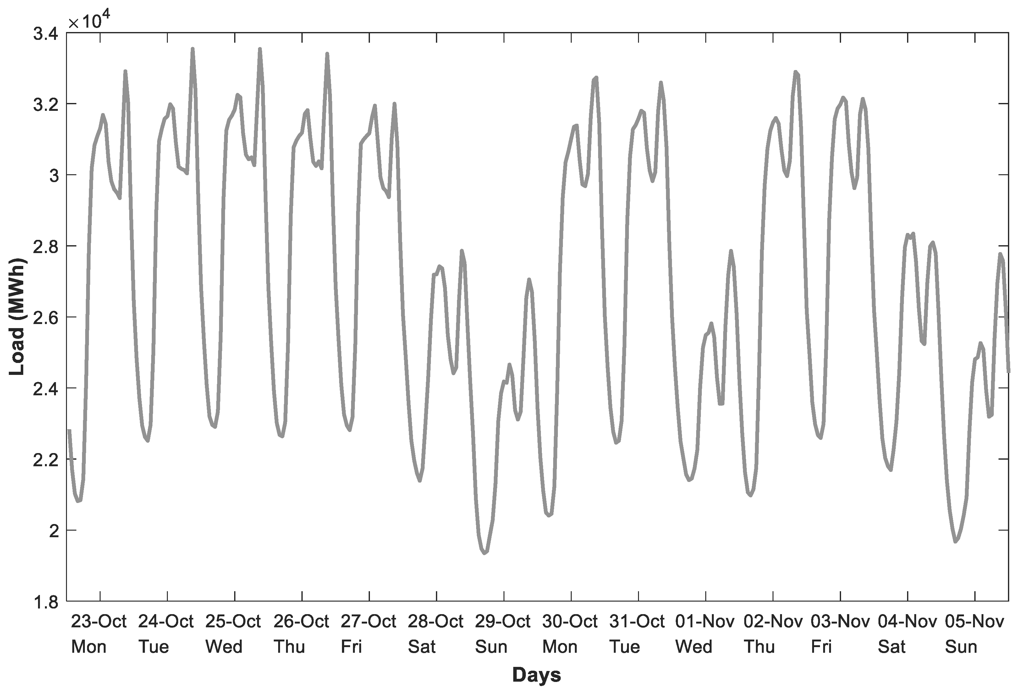
One issue that has not received as much attention as the forecasting engine is the forecasting of special days. Several days throughout the year show a profile that does not match the expected profile for its weekday. These differences may be caused by temperature [26] but, the more extreme cases are caused by socio-economic effects of the calendar. In Figure 1, we can see how the load profile for a special day (1 November, a national holiday in Spain) has lower demand values with respect to any normal day. This and other special days are harder to forecast and incur higher forecasting errors that increase forecasting losses. This is especially important because a low average forecasting error with large peak errors may be costlier than a slightly less accurate forecast that has smaller peak errors. This research focuses on how to provide the proper information about these special days so that a forecasting engine may be able to forecast them more accurately.

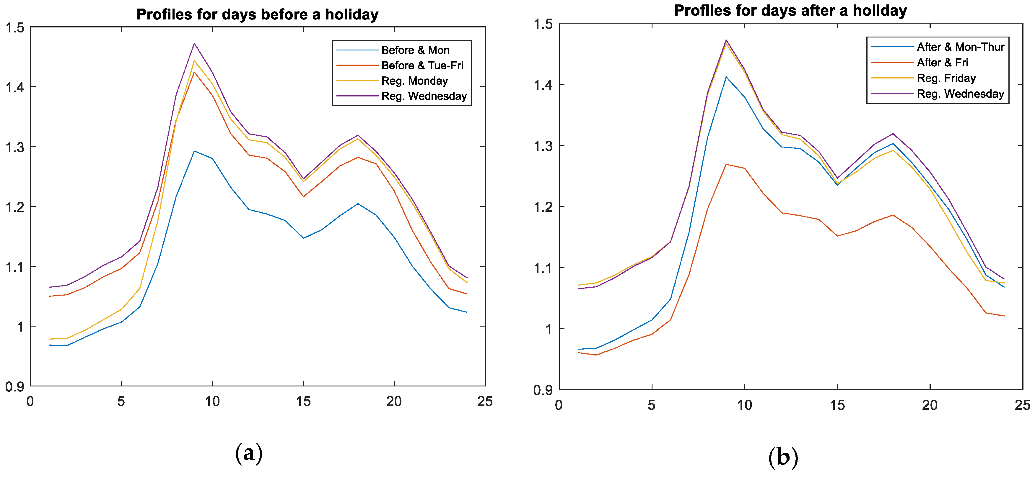
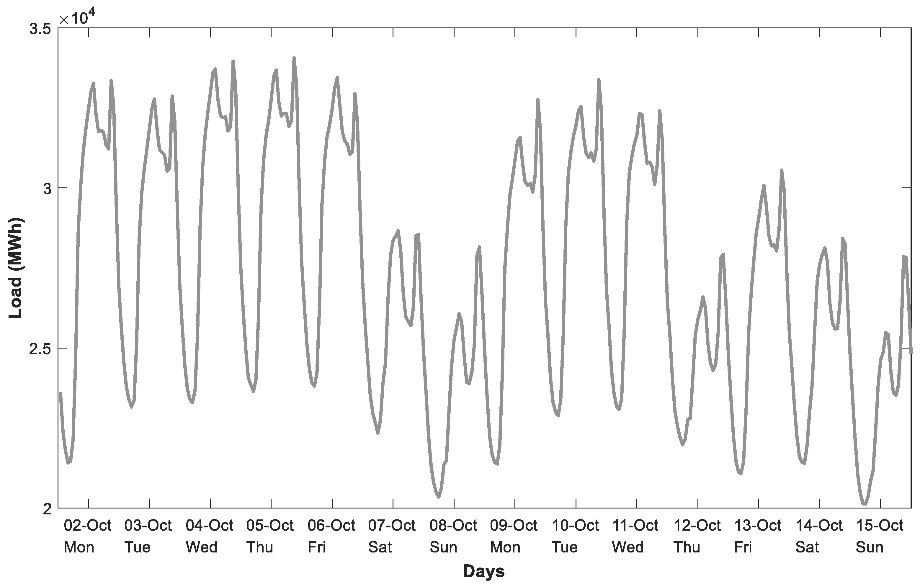
There are several ways in which the calendar affects load profiles. Figure 1 already shows that a national holiday has a profile more similar to a Sunday than to a typical weekday. However, this does not mean that all national holidays share the same profile. In addition, the demand pattern of normal days can be altered by the proximity of special days (see Figure 2) such as the Monday before a holiday or the Friday after a holiday. The load profiles of special days do not have the same demand pattern, it can be seen in Figure 2 that the load profile of 12 October is different to the load profiles of normal days. In addition, the demand pattern on 13 October is lower than the demand pattern of a normal Friday, which is because it happens after a holiday. If we consider all special days belonging to only one kind of day, the accuracy of the demand prediction will be affected.

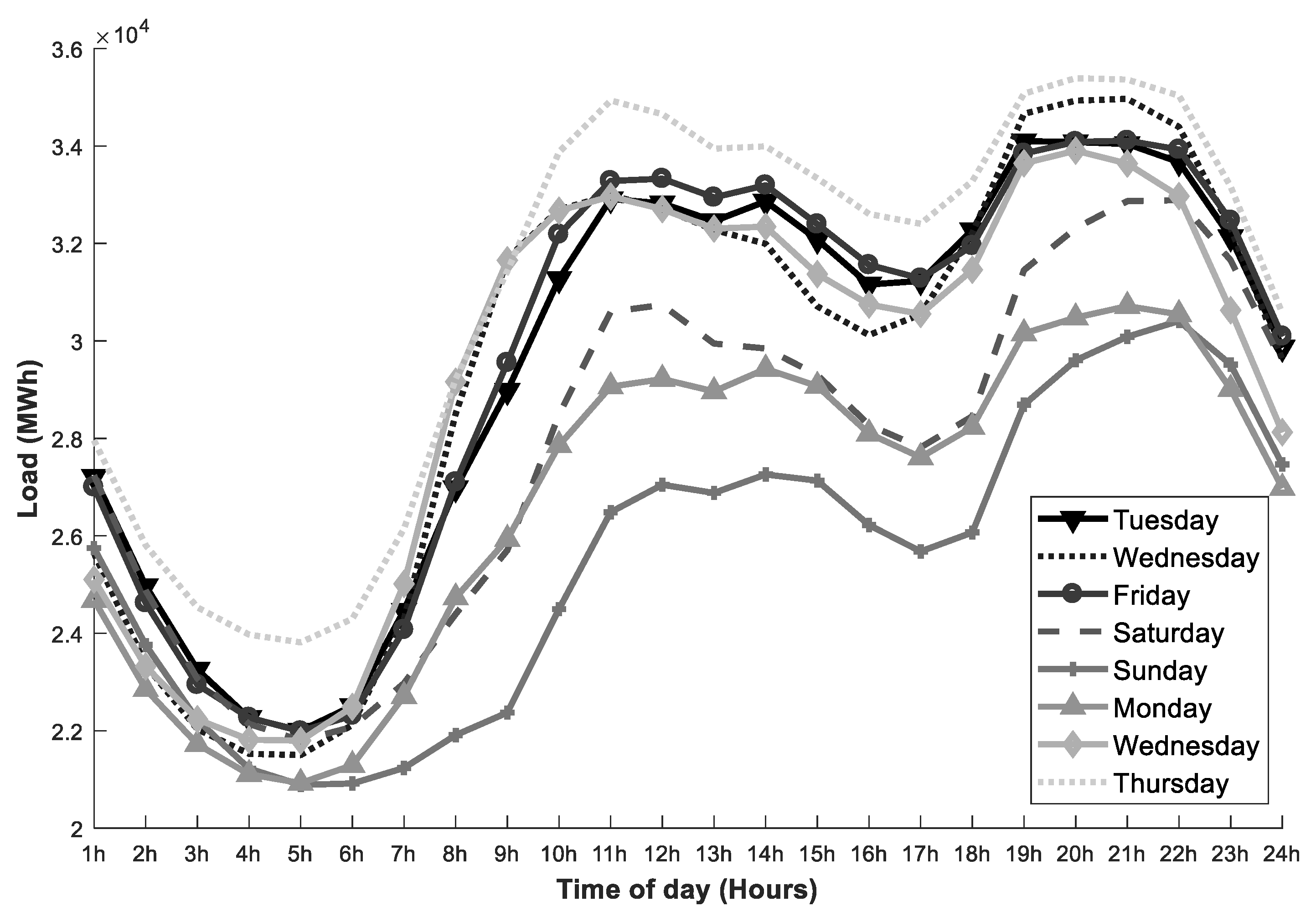
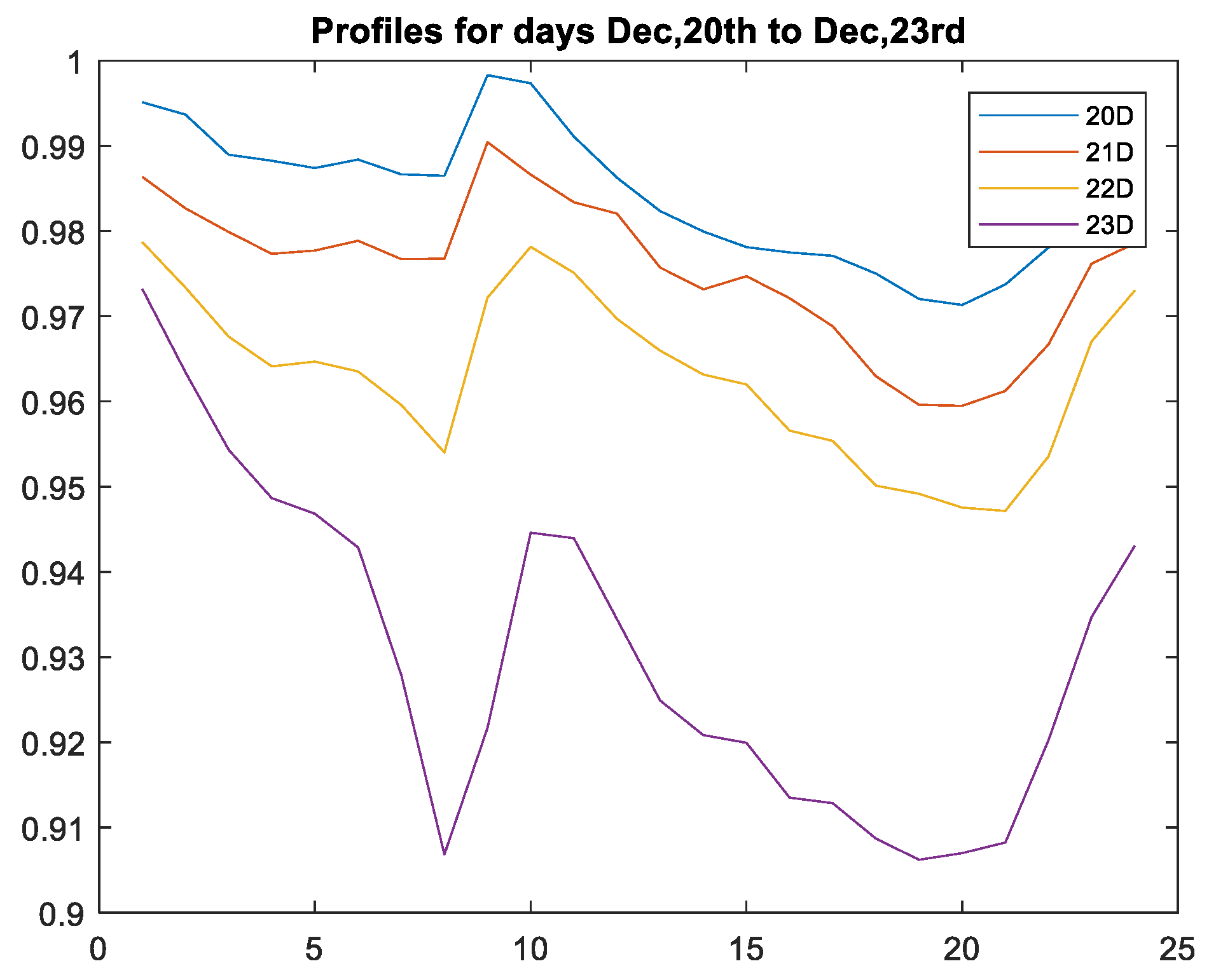
Each day of the week may have its own profile and, in many cases, there are interactions causing the type of special day to be conditioned by its weekday. The same special day may have different demand patterns depending on the day of the week. Figure 3 displays the profile load of the special day 7 December for the period 2010 to 2017. The day before and after 7 December is a holiday. However, the demand load for Monday, Saturday and Sunday are very different from the other days, as well as the first hours of Thursday and the period between 9 am and 7 pm on the same day. Special days are classified into several types depending on the day of the week.

However, this classification of special days is not enough to obtain all the information that lies within the profiles of the special days. A deeper classification of the special days is necessary to improve forecasting accuracy, which has been the subject of this work. All demand patterns different from the demand patterns of normal days should be analyzed, taking into account the influences on demand described in this paper. Special days with similar demand patterns are grouped to reduce the complexity and computing times of the forecasting model.

The contribution of this research line in:

• This paper proposes a classification for special days that includes more than 40 types of day, while most published articles limit their classification to 15 or less.
• The performance of this classification is tested against less extensive classifications, proving that its use provides a more accurate forecast for each type of day.
• Non-linearities present in special days load profiles are overcome by using separate models for each hour and categorical variables for each type of day.
• A detailed analysis of special days in Spain is provided, which can help to replicate this classification in other systems.
• The benefits of this approach stem not only from the reduction of the average forecasting error but especially on the reduction of error peaks which usually happen on these special days.

This paper is organized as follows: Section 2 describes the state of the art and previous work related to forecasting special days. Section 3 shows the available data for the analysis, the characteristics of the mathematical model used, the treatment to the input variables in order to be processed by the model and the different experiments carried out. Section 4 includes the results of these experiments, analyzing how each classification of days affects modeling accuracy. Section 5 is a brief conclusion expressing the relevance of using complex classification schemes for the different types of days in order to achieve accurate forecasts. Appendix A and Appendix B include a more extensive review of the results.

2. State of the Art and Related Work

The aim of this study is to improve STFL accuracy for special days by defining a more detailed classification. Load profiles of the different days do not follow the same pattern and if we group the most similar demand patterns, the accuracy of the prediction will increase. Demand patterns of special days and demand patterns of normal days are very different. If our forecasting model does not differentiate between normal and special days, the results obtained will be inaccurate on these special days.

In most of the research works related to STFL, all days are classified into two or three large groups such as weekdays, weekends and holiday periods [23,35,36,37]. Some research articles, where special days are classified according to the demand pattern, they are grouped into 5 [38] and 15 [39] different days, obtaining better results than choosing only three types of days. The profile loads on special days do not have the same demand pattern (i.e., days adjacent to holidays, period of Christmas, Easter, national holidays, week before Christmas) [26,38], consequently the forecasting uncertainty is greater for these days. The day of the week is also an important factor in the load profiles of special days [40,41,42]: the same special day may have different demand patterns depending on the day of the week. In addition, demand pattern of normal days can be altered by the proximity of special days [38,40,41,43].

Several works have been published for anomalous load forecasting [26,38,39,40,41,42,43,44]. In the case of research [42], it only takes into account the days with the greatest errors in the prediction. These days are the holidays that fall on a Saturday or a Monday. This research was done in Korea where Sundays are holidays. Special days are classified into four categories (Tuesday, Wednesday, Thursday and Friday; Saturday; Monday; Sunday). This research only classifies special days depending on the day of the week they fall on. This method reduces the highest prediction errors. However, the accuracy of the prediction can be improved if a deep classification of special days is performed. In [43], the different types of day are classified based on the shape of the load curve into three categories (weekdays (Monday to Friday); Saturday; Sunday and Holidays). Due to the application of special rules, the proximity of the forecast day to a holiday is taken into account. This classification does not differentiate special days from each other. In [26], data are classified according to the type of day and month, to capture the effects of seasonality on the load profile. In addition, three variables are added to check the impact on electricity consumption of holidays, days following a holiday and Easter. In [38], special days are classified into five different types of day (weekday, Saturday, Sunday, Monday and special holidays), but a neural network is necessary for each type of special day. In addition, a fuzzy inference model forecasts the maximum and the minimum loads of a special day. Therefore, if the number of types of special days increases, the forecasting model will be more complex. In [39], SOM is used to group the days with similar load profiles and STFL is performed by means of an NN. SOM performs the classification of the different types of days into groups that can vary between 11 and 15. This technique has been discarded, because the separation of the different types of days requires prior knowledge that is difficult to assemble and whose result is not clear. The classification proposed in this research is similar to the classification described in [40]. Special days are treated according to whether they fall on the same date, the same day of the week, the day of the week is weekday or weekend. However, the classification of special days must be greater as well as the number of days considered as special days. In [41], a variation of the forecasting model described in [40], is used, increasing training period to 8 years and formulating a specific rule to be applied in France. However, the classification of special days into seven categories is still insufficient. In [44], special days are classified into four categories such as common holidays (some national holydays and all local and regional holidays) and three special national holidays.

The use of categorical variables to formulate such classifications in linear regression models is very common [26,41,44,45,46] and it is the same approach used in this paper. These categorical variables define the type of day and are translated into dummy binary categories that allow the regression model to estimate each type of day individually without any linear assumption among normal or special days.

3. Methodology

The starting point of this study is a load forecasting system currently in use at the Red Electrica de España (REE) headquarters. REE is the Transport System Operator for the Spanish system. The following paragraphs aim to describe the available data, the variables actually introduced in the system and the mathematical aspects of the model. In addition, this section will describe the different experiments carried out to determine how the variety of special days can be classified and the type of information used to characterize each type of day.

3.1. Available Data

The input data can be grouped as load, temperature and calendar data:

• Load: The load data are hourly values from the whole Spanish inland system. Data covers the period 2010 through 2017. The data have been filtered to discard incoherent outliers and fill in missing data. Only 0.01% of the data points were affected.
• Temperature: The temperature data consists of maximum and minimum daily values from 59 stations scattered throughout the country. As described in [24], only the most relevant locations are actually included in the model.
• Calendar: The information on special days is initially extracted from the B.O.E. (National Official Gazette) [47]. This document includes all national and regional holidays for each year. However, even though these dates present a specific load profile, they are not the only ones that need special treatment and, therefore, additional information will be needed to establish a definite classification of special days. This additional information can be extracted from the characteristics of the load but in this case, the forecasting model was designed by an expert in the field.

3.2. Mathematical Model

The forecasting model used as starting point is thoroughly described in [24]. It includes a neural network and an autoregressive model whose output is combined to provide a single forecast. The combination of both outputs is more accurate than both of them, therefore, both techniques have advantages and are useful as forecasters. However, the black-box characteristics of the neural network makes it less useful to extract conclusions about the model and it is consequently discarded for this study. In addition, the limitation that regression models impose of linearity between each variable and the output can be overcome by linearization methods (temperature) or other techniques. The abnormalities that special days cause in the daily profiles are non-linear because each hour is affected differently and, therefore, the resulting profile is not a scaled copy of the profile of a regular day. In addition, there is no linear relation between the nature of each special day and its effect on the load. The regression model used allows us to include these abnormalities by using individual models for each hour, whose coefficients, therefore, are not restricted in any way and by using separate binary categories for each type of day. The model then provides specific profiles for each category without any relation between the hours within a profile or between profiles of different categories.

The autoregressive model is described by Equation (1), where a given output y_t is a linear combination of the model’s p previous known errors (e_t-i), a number of exogenous variables included in X_t and a random shock ε_t:

$$y_t={\displaystyle \sum }_{i=1}^p{\phi }_i·e_{t-i}+X_t·\theta +{\epsilon }_t$$

(1)

This type of process is useful for characterizing time series which are self-correlated to some extent. However, the autoregressive part may also cover up the effect of the exogenous variables. Therefore, in our study, the autoregressive part of the model has been eliminated as shown in Equation (2):

$$y_t=X_t·\theta +{\epsilon }_t$$

(2)

The effect that any exogenous variable may have on the load may vary throughout the day, which means that the coefficient for each variable may take different values at different times. In order to meet this requirement, the 24 h profile is obtained by using one model for each hour. The input structure for each model is the same. In addition, the output used is the natural logarithm of the load, which experimentally shows a lower modeling error than the actual load.

3.3. Input for the Model

The exogenous variables used in the model stem from the available data described above. However, due to the non-linearities present in most load-variable relations, a pretreatment is necessary to conform the definite variables going into the exogenous variables matrix:

• Load: The initial model contained two variables used to model the long-term trend as a quadratic function of time. This approach may be valid for shorter periods of time (3 years) but for longer periods, the long-term behavior is not reproduced by a quadratic function. Therefore, these variables are substituted by a 52-week moving average of the previous load for each model. In addition, the initial model included the last known load value at the time of the forecast. This variable, as mentioned above about the autoregressive terms, may hide the effect of other variables like temperature or special days. Therefore, it is also removed from our study.
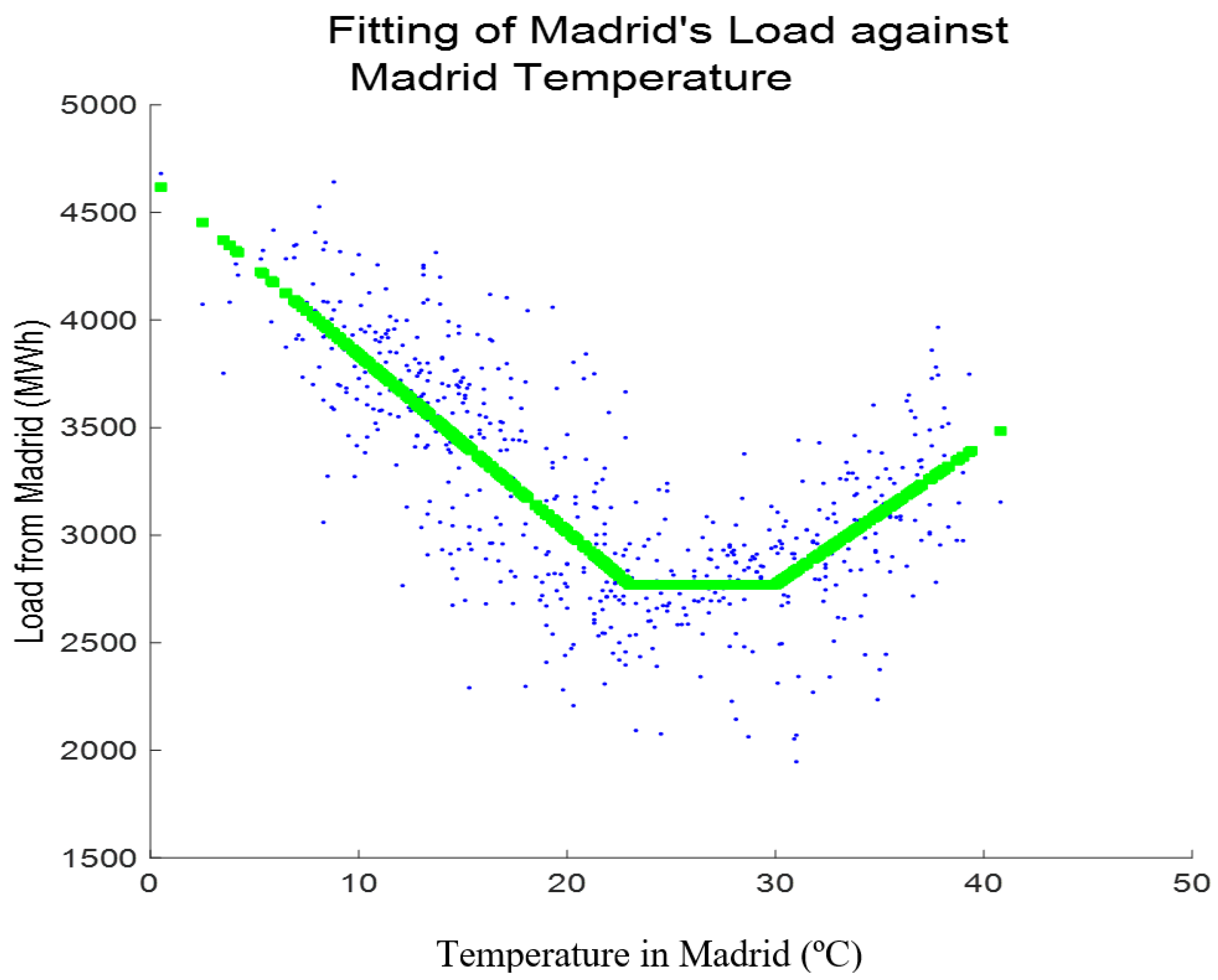
• Temperature: The effect of temperature is non-linear as both hot or cold temperatures cause an increase in electricity consumption. Moreover, it has a certain inertia and temperature during previous days also has an influence on current demand. In addition, for large regions with a diversity of climates, it is not desirable to use a calculated average temperature for the whole region as it masks the extreme temperatures that may trigger high demands locally. To account for all these factors, the temperature variables are first selected from all available locations: Only 5 (Madrid, Barcelona, Seville, Bilbao and Zaragoza) of the 59 available series are used representing the different climate areas in Spain. Linearity is achieved by using the Hot and Cold Degree Days (HDD, CDD) method [44].This technique splits the data series into two different series each one accounting for demand increases for hot and cold temperatures. It requires defining two thresholds splitting the temperature range into three parts: cold days below the cold threshold, neutral zone in between thresholds and hot days above the hot threshold. Therefore, this method models the load-temperature relationship as a piecewise linear function that calculates different slopes for cold and hot days while it sets the slope for the neutral zone to zero. Figure 4 illustrates this methodology.
  In order to model temperature inertia, the model includes the current value and lagged variables from all locations for the last two days. To sum up, the temperature variables include HDD and CDD series from five locations with the current and two lagged values. This treatment adds up to 30 variables.
• Calendar data: The information about the type of day is critical as load profiles vary greatly from regular Mondays, to Fridays, Sundays, and even among holidays and special periods throughout the year. Therefore, a detailed classification is key to forecasting these special days accurately. In the starting model, 53 variables are used to classify the type of day along with eleven more to assign the month. The variables included in the model from these 53 variables are described in

  Table 1. National special days.

  Type 1 (6)		Type 2 (5)		Type 3 (13)
  All instances are included regardless of the day of the week. (6 variables)	1 Jan	Only whenever the day of the week is Mon-Fri. 1 (5 variables)	2 Jan	Each day from Mon. before Good Friday to Sat. after Easter Monday (13 variables)
  	6 Jan		5 Jan
  	1 May		7 Dec
  	24 Dec		26 Dec
  	25 Dec		30 Dec
  	31Dec

  ¹ Weekend instances may qualify into other categories.

  ,

  Table 2. Regular national holidays.

  Weekend	Monday	Tuesday-Friday
  Days included as holidays in BOE:		Typically:
  		15 August
  		12 October
  		1 November
  		6 December
  		8 December

  ,

  Table 3. Days before and after a holiday.

  Before		After
  Tuesday to Friday	Monday 1	Monday to Thursday	Friday 1

  ¹ Typically, the profile is more affected if the day is in between the weekend and the holiday.

  ,

  Table 4. Periods affected by Christmas.

  Week before Christmas Day	Week after Christmas Day	Week after New Year Day
  Four variables 1 each for one day:	One variable for days only Monday to Friday	One variable for days only Monday to Friday
  20 December	27–29 December	2–5 January
  21 December
  22 December
  23 December

  ¹ Days from the week before seem to be differently affected among them while the days in other periods are all equally affected within their own period.

  and

  Table 5. Types of day category summary.

  Type of Category	General Description	Specifics	Number of Variables
  EXCLUSIVE	Special days with specific profiles	Easter	13
  		Any day of the week	6
  		Only weekdays	5
  	National holidays with generic profile	Weekend	1
  		Monday	1
  		Tuesday to Friday	1
  	Days adjacent to holidays	Before	2
  		After	2
  DAYS OF THE WEEK			6
  MODIFIERS	Christmas periods	Before Christmas day	4
  		After Christmas day	1
  		After New Year’s day	1
  	Summer vacation (August)	Week number	3
  	Regional holidays	GNP fraction	1

  .

A set of 24 variables is used to identify 24 specific days that are considered to have a profile of their own, incompatible with any other day. These cases are described in Table 1:

The three variables used to classify the rest of national holidays from the B.O.E. are described in Table 2:

Days adjacent to a holiday or special day may show a different load profile depending on the day of the week. Table 3 shows the four variables used to model this phenomenon.

The classification of regular days is done through six variables for days Monday to Saturday. Variables from Table 1, Table 2 and Table 3, described categories defined as exclusive: each day belonging to any of these categories may not belong to any other. However, the following categories are thought of as modifiers to the day of the week and may be active at the same time as the day of the week.

Religious holidays are widely observed in Spain and the work and school calendar includes two periods besides the summer-time in which people concentrate their vacation days. The effect of Easter was included in the exclusive variables because, by definition, it happens on the same weekday every year, however, the period around Christmas presents a complexity that forces the use of the following modifiers shown in Table 4:

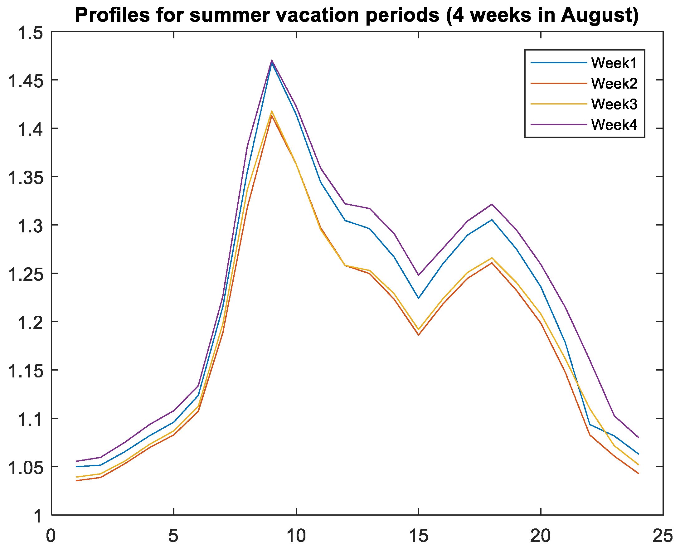
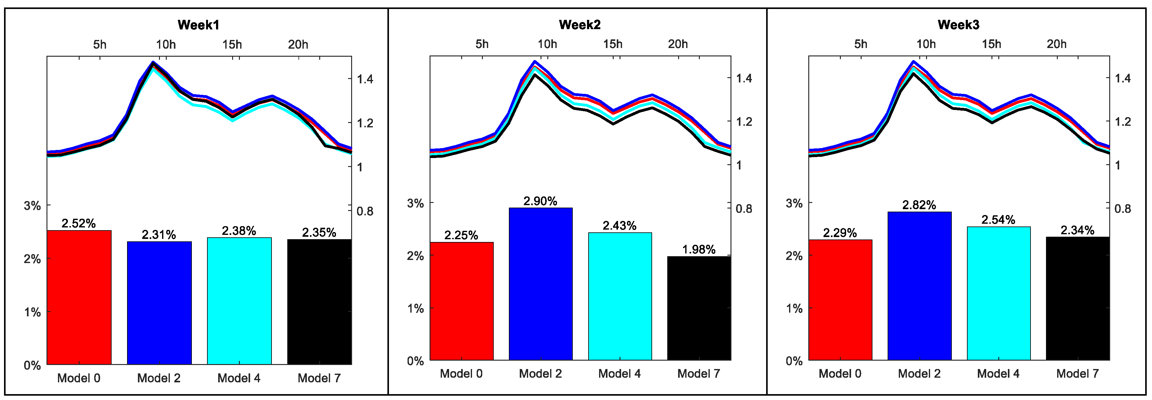
The summer period is affected by a lower demand from industry due to holidays but a higher demand from services due to tourism. This fluctuation is not constant throughout the summer, but may vary weekly. The inclusion of the month variables helps modeling this behavior but, in the case of August, three additional variables have been added to model differences among weeks.

Finally, regional or local holidays are published in regional gazettes and identified by a variable which, in this case, is not binary but equivalent to the fraction of the National Gross Product that the particular region represents.

The effect of Daylight Savings Time is also considered in the initial forecasting model in two ways. Firstly, it relies on the autoregressive part to phase out the error from the time shifts in March and October and secondly, in order to ease the transition, the first three days from each season are considered as special. These special days are not considered in this study because the autoregressive part is removed. To sum up, Table 5 summarizes all variables for the type of day.

In summary, the model includes one long-term load variable, 30 temperature variables, 11 binary variables for the month and 53 binary variables for the type of day. The output variable is the natural logarithm of the load.

3.4. Experiments and Results

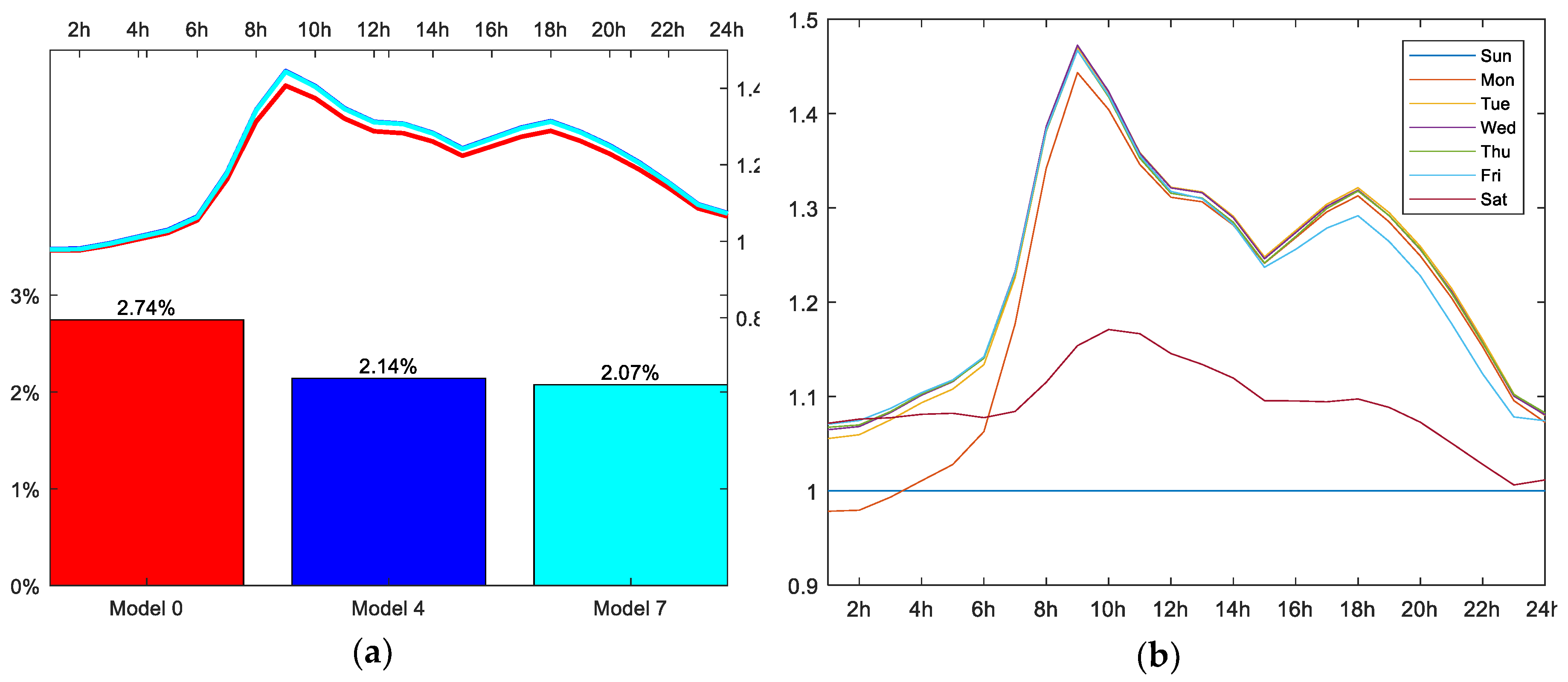
The aim of this study is to determine the different load profiles that a given day may have depending on social- and labor-related characteristics. To determine whether the classification above is adequate, simplistic or overly complex, this study proposes a series of tests to determine how the accuracy of the model varies as the complexity of the classification increases. These experiments are based on eight different classifications starting from the most simplistic, in which only the day of the week is observed and finishing with the most complex, in which all categories described above are considered. The different models are incrementally defined in

Table 6. Summary of incrementally complex models.

Number of Model	General Description
0	Only six variables are included which are used to describe the day of the week.
1	Three variables are added	Holidays	Type 1 of special holidays, Maundy Thursday, Good Friday, Easter Monday and all regular national holidays
		Days before holidays	Jan 5th, Dec 7th, Dec 30th, Good Wednesday and all days from the before-holiday final category
		Days after holidays	Jan 2nd, Dec 26th and all days from the after-holiday final category
2	Five variables are added	Regional	As described in the final classification
		Week before Christmas	Dec 20th to Dec 23rd in one single category
		Week after Christmas	Dec 27th to Dec 29th in one single category
		Week after New Year’s	Jan 2nd to Jan 5th in one single category
		Easter	Monday and Tuesday prior to Good Friday and Wednesday to Saturday from the next week
3	One variable added	Summer holiday	First three weeks of August
4	Four variables are added	Holidays is split into three categories	Holidays I.P.M. that happen on weekend
			Holidays I.P.M. that happen on Monday.
			Holidays I.P.M. that happen on Tuesday to Friday
		Days before holidays is split into two categories	Days before holidays I.P.M. that happen on Monday.
			Days before holidays I.P.M. that happen on Tuesday to Friday
		Days after holidays is split into two categories	Days after holidays I.P.M. that happen on Friday.
			Days after holidays I.P.M. that happen on Monday to Thursday
5	Thirteen variables are added	Easter	Easter I.P.M. each day gets its own category (6)
			Saturday and Sunday after Good Friday each get their own category (2).
		Week before Christmas	Dec 20th to Dec 23rd each get their own category (3)
		August	Each week gets its own category (2)
6	Eleven variables are added	Specific holidays	All type one (6) and type 2 (5) national special days are assigned their own category. (11)
7	Four variables are added	Easter	Wednesday, Thursday, Good Friday and Easter Monday each get their own category (4)

, in which each incremental change is described.

Special days are scarce and certain types may only happen every two or three years. This causes a problem when splitting the data set into training data and out-of-sample testing data. In order to solve this, all experiments have been carried out using each one of the 8 years as the testing period and the other 7 as training data. Therefore, the results provided for each model correspond to an 8-year period for which every year is obtained as an out-of-sample test of the model trained with the other 7 years.

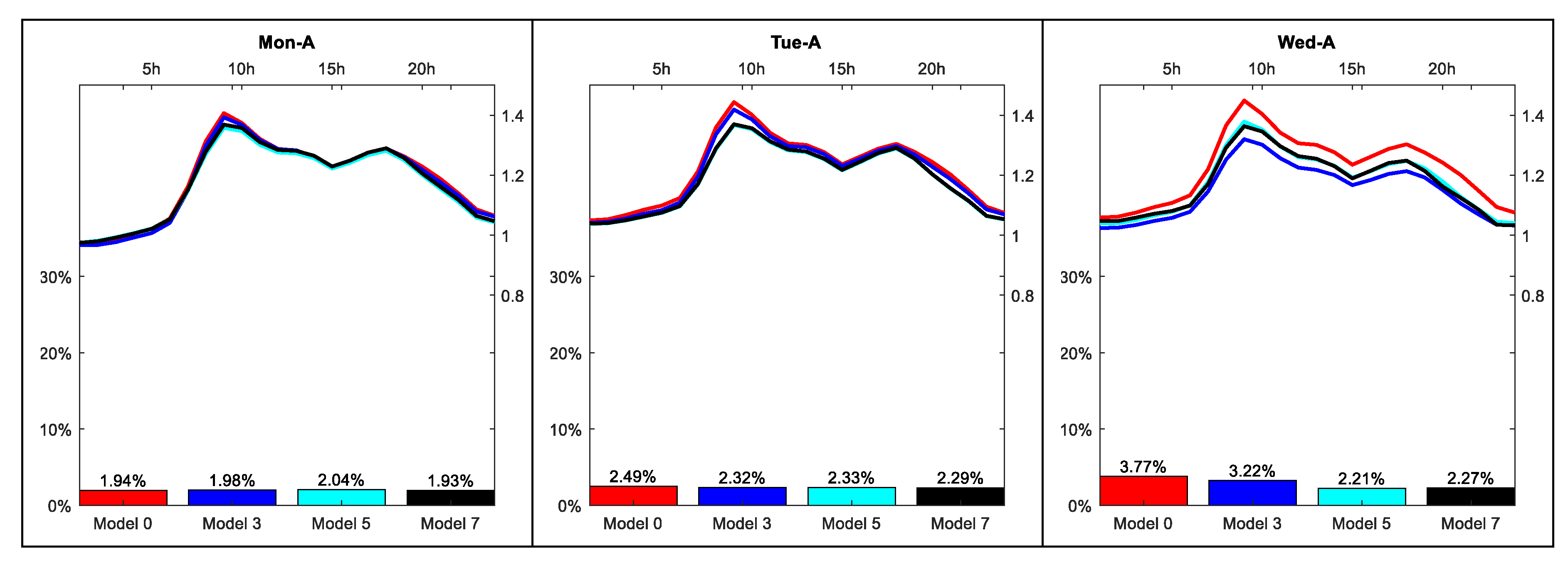
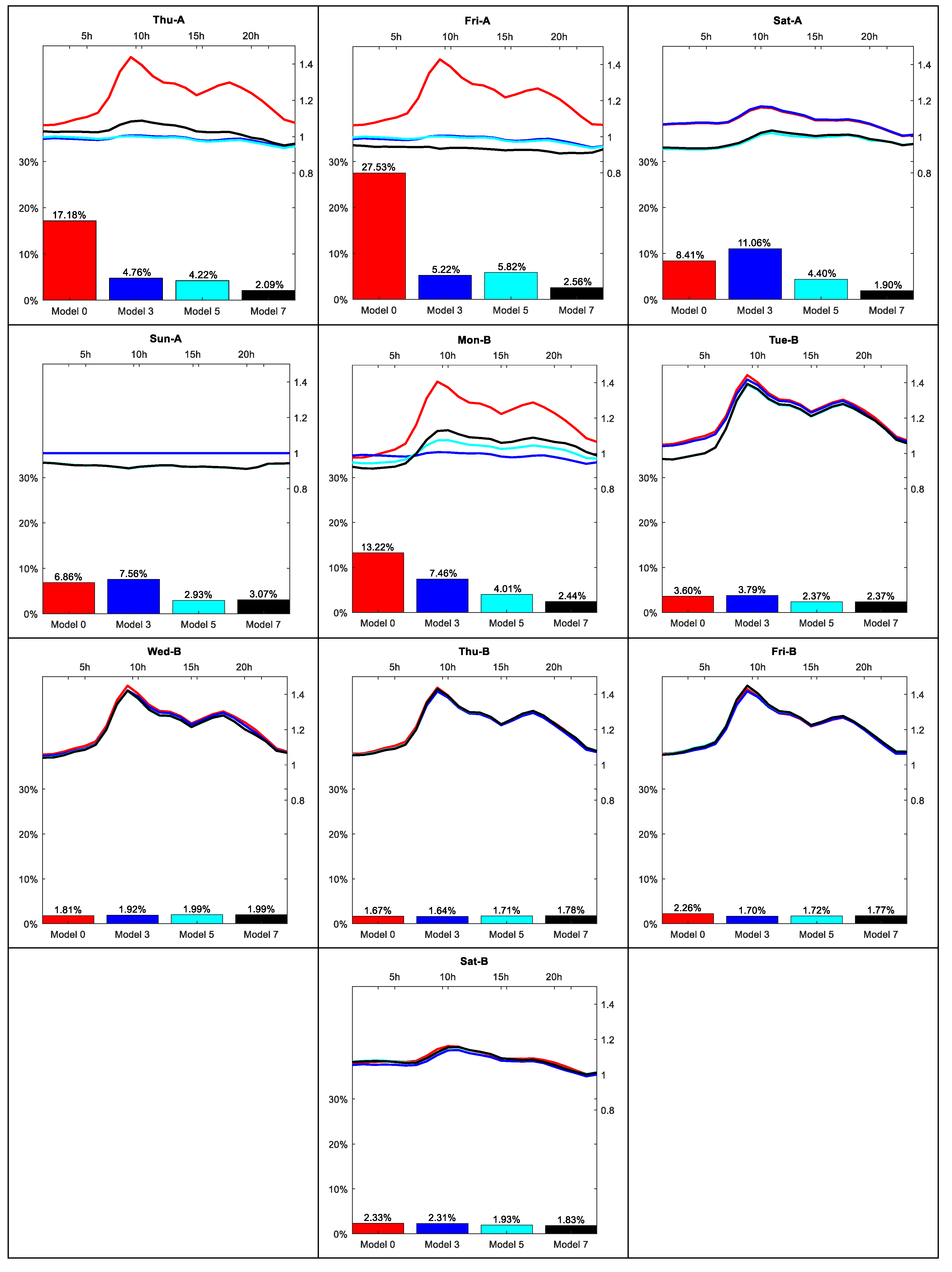
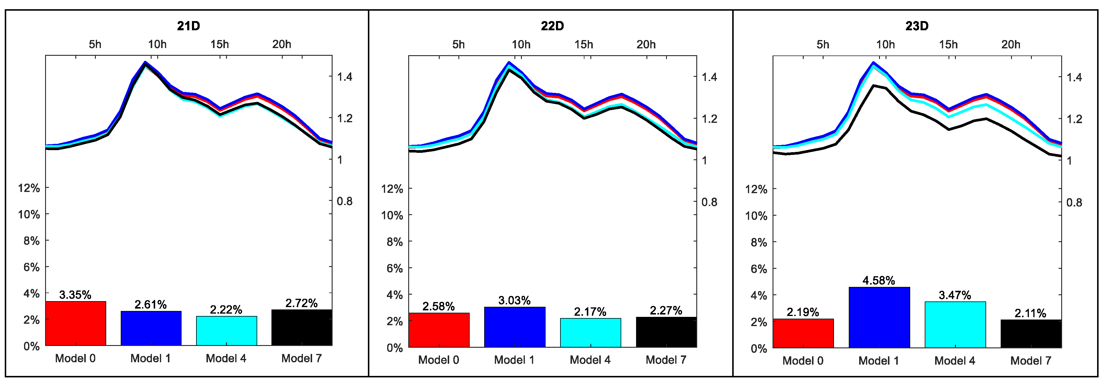
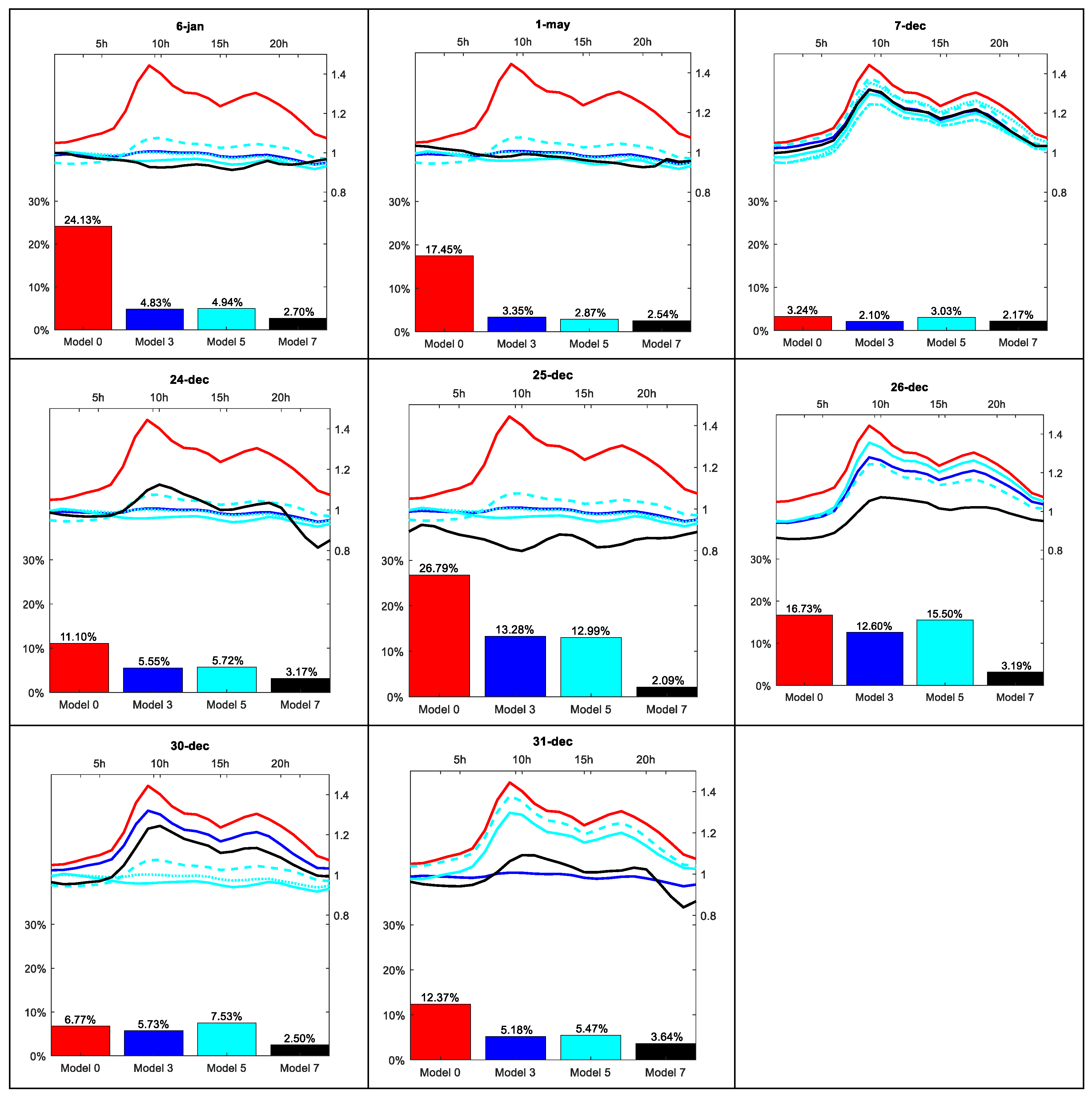
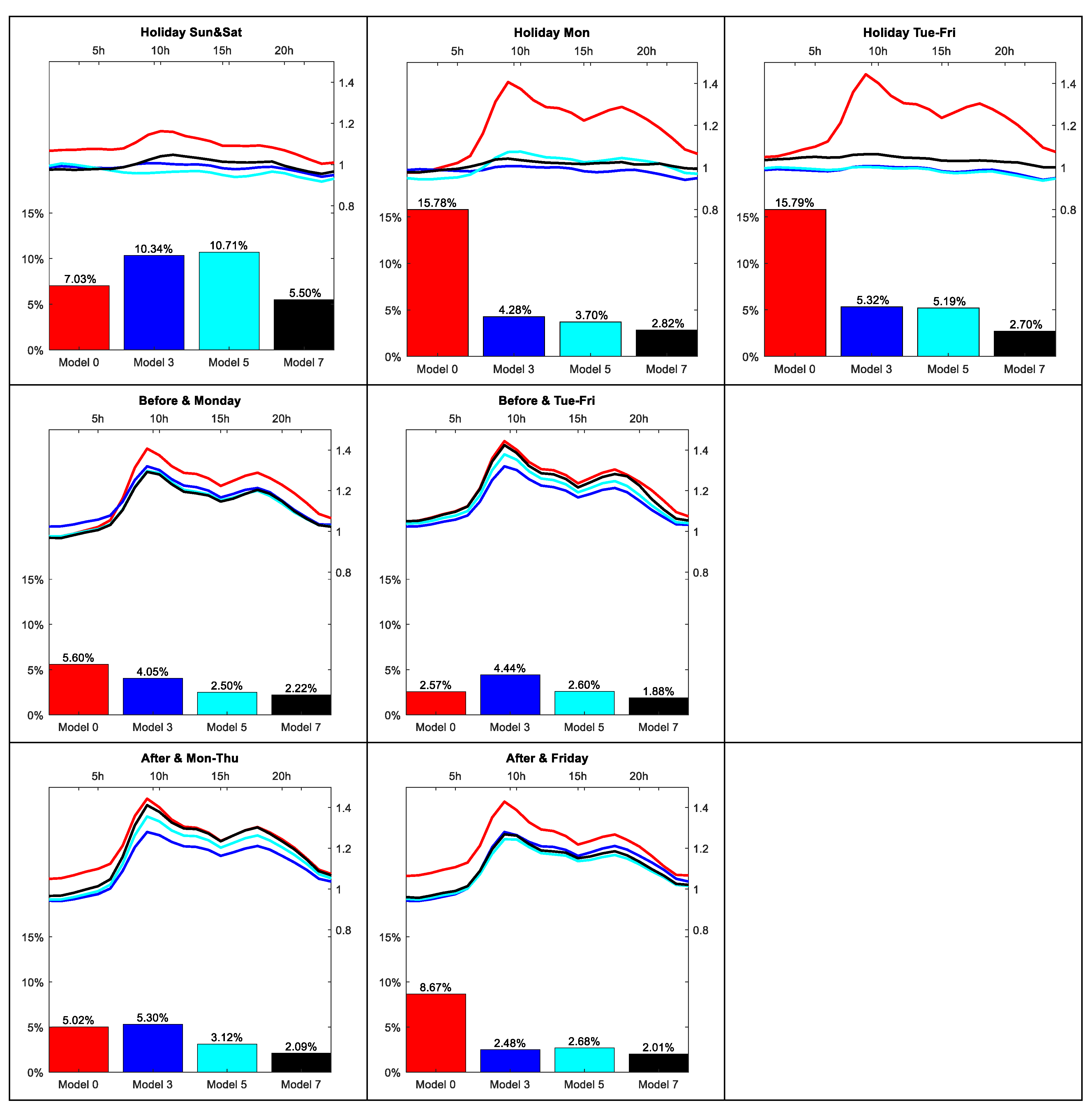
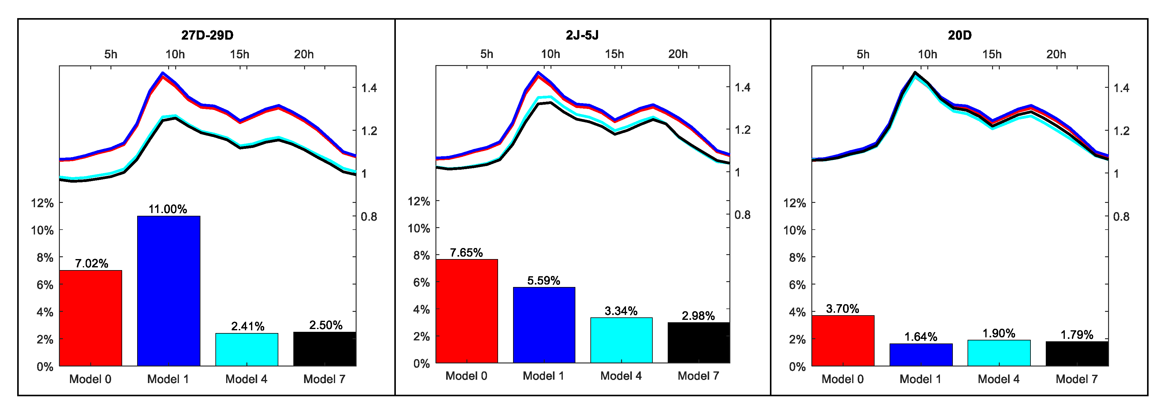
Each model provides a different output which differs especially on days for which other models use a different classification. It is obvious that when a model includes a new category to better suit a type of day, the days falling under said category are expected to be more accurately modeled. However, it is worth mentioning that by “cleaning up” the category in which these days were before, the remaining days in the category also experience a change in their profile that should be for the best. Therefore, even among models that apparently have the same definition of a category, i.e., all models have a regular Monday category, there may be differences in these categories among these models.

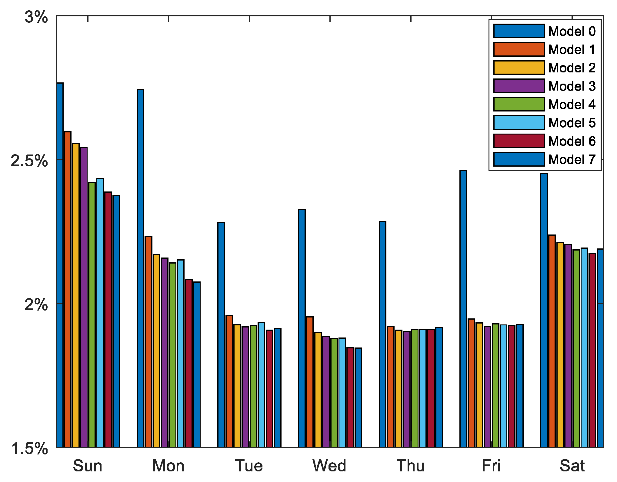
The measure of reported error is the Mean Average Percentage Error (MAPE) and it is categorized by type of day to focus on the specific changes among models. For each general category of type of days, the error from each model that introduces a significant change in the definition of said category is reported. Models that treat a category in the same way and that may only experience collateral changes are not reported for clarity reasons.

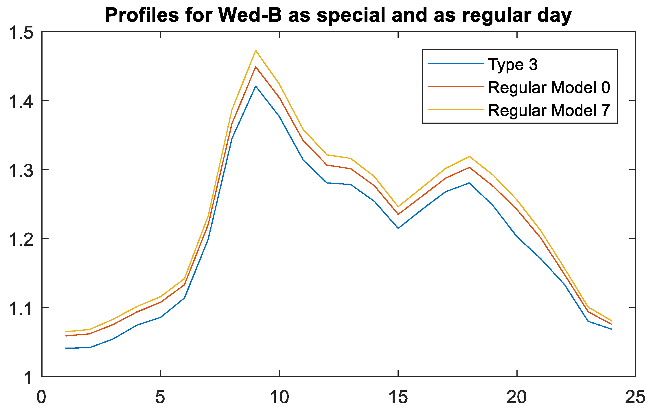
In addition to the accuracy of a given classification, it is important to understand how each classification models the load profile. This will help us in determining not only which classification is more accurate but also, and more importantly, how each special day’s profile is different from each other and learn the expected load from each of them.

Since the output of each model is not the actual load but the natural logarithm, the effect of each coefficient on the load can be considered not as an addend but as a multiplier to the expected load. Considering the way that the type of day categories are defined, the base profile is that of a regular January Sunday. Therefore, a category coefficient higher than 1 means that the typical load at that particular hour for that particular category is larger than the load expected for a regular January Sunday controlling for other factors like temperature.

The coefficient profile calculated for each category by each model is the second result of this study and it provides a useful tool for understanding the nature of each type of special day and the behavioral changes of the consumer on such types of day. These profiles are included in the results section if they are relevant but all of them are also included in Appendix A for the reader’s reference.

4. Results

The following section describes the results obtained by each model for every category of type of day. These results include the MAPE results for each model to assess the accuracy improvement that the refining of each category adds to the model. In addition to the error, it also includes the coefficient profile so that the accuracy change can be interpreted based on how the category is differently modeled.

4.1. Regular Days

Even though the aim of this study is not regular days, it will help understand the rest of the results if this category is analyzed. The definition of the category remains unchanged through all eight models; however, more and more special days are removed from the category from model 1 to model 7 and, therefore, the modeling of regular days is more accurate. Figure 5 shows the changes in MAPE on each day of the week through all models. The largest improvement occurs from model 0 to model 1. This model is the first one to acknowledge the existence of special days. Nevertheless, accuracy increases continuously through model 7, especially on Sundays, Mondays and Saturdays.

The change in the models can be seen in Figure 6a, in which the load profile and the reported MAPE for each model is shown for regular Mondays. The graph shows how the model 0 profile is lower than the other two, which are essentially equivalent. This is because model 0 models regular Mondays after all Mondays in the data set while models 4 and 7 exclude most or all special days, which have a lower profile. The rest of the regular days’ results are shown in Appendix A (Figure A1). In Figure 6b the profile for all days of the week from model 7 can be seen and how Monday has a lower start while Friday has a lower finish. Saturday has a unique profile and Tuesday, Wednesday and Thursday are very similar.

It is also important to quantify whether two profiles are similar enough to be considered the same type of day. In order to do so,

Table 7. Differences between days of the week.

Date	Sun	Mon	Tue	Wed	Thur	Fri	Sat
Difference	17.11%	8.27%	0.93%	0.57%	0.57%	3.26%	17.11%
Most similar	Sat	Tue	Wed	Thur	Wed	Thur	Sun

presents the maximum difference between each profile and its most similar pair. This measure expresses the difference between the profiles for two types of days. Specifically, it is the maximum percentage difference between the two 24 h profiles. It is a measure of how two profiles may or may not be equivalent and represent the same type of day. Both type-of-day categories are named at the top and bottom of the table. In this case, there is less than 1% difference between Tuesday, Wednesday and Thursday and, therefore these three categories are candidates for a joint category.

4.2. Special Days Type 1 and Type 2

Special day types 1 and 2 include 11 fixed dates (see Table 1) that are considered to have specific load profiles. The models that introduce differences into these categories are 0 (all days are regular days), 3 (includes holidays and days before and after), 5 (distinguishes profiles for different days of the week) and 7 (each day is considered unique). Figure 7a shows the model accuracy of the category in these four models. Including these categories as general holidays or before/after holidays lowers the error from 15.6% to around 7%, but then considering each individual holiday yields a much better result of 2.8%. For these special days, assigning different profiles according to the day of the week (model 3 vs. 5) does not improve the result.

In addition, Figure 7b shows the example of Christmas day and how the coefficient profile changes in each model for this particular day. It is interesting how Christmas day shows a much lower load profile than most other special days and so it needs to be considered apart. The coefficient profile and error graphs for the rest of days within the category are included in Appendix A (Figure A2). The maximum difference between the most similar profiles is detailed in

Table 8. Differences between special days type 1 and 2.

Date	1 Jan	2 Jan	5 Jan	6 Jan	1 May	7 Dec	24 Dec	25 Dec	26 Dec	30 Dec	31 Dec
Difference	5.79%	11.2%	10.2%	6.65%	6.65%	10.2%	3.43% 1	5.79%	11.9%	10.8%	3.43%
Most similar	25 Dec	7 Dec	7 Dec	1 May	6 Jan	5 Jan	31 Dec	1 Jan	31 Dec	7 Dec	24 Dec

¹ The most similar profiles belong to 24 Dec and 30 Dec, but the peak difference is almost 3.5%.

and it shows that all profiles are independent.

4.3. Special Days Type 3

Special days type 3 include the Easter period. Each day is considered to have its own profile but differently from types 1 and 2, these days do not happen on the same date each year. The models that affect this type of days are 0, 3, 5 and 7 and the overall accuracy for these days is shown in Figure 8.

This type of special days includes some whose profile is deeply affected, like Good Friday, and others, like the Wednesday after Easter Monday, that are only slightly different to a regular day. Figure 9 shows the coefficient and error graph for these two examples while the rest are included in Appendix A (Figure A3). For clarity reasons, days that happen in the same week as Good Friday are from now on referred to as A, while those that happen on the next week will be known as B.

While Figure 9a shows how accuracy on Good Friday increases as the classification is more complex, it does not happen the same way for the next Wednesday, as it is shown in Figure 9b. This may lead to the conclusion that such a Wednesday should not be considered special, as model 0 yields the most accurate result. However, as aforementioned, the profiles for regular weekdays from model 0 are lower than actual regular days due to the presence of holidays that, in that model, are considered regular. The MAPE for such Wednesday if it was considered as a regular day in model 7 would go as high as 3.3%. Figure 10 shows these profiles and illustrates how the profile for that specific Wednesday is lower than both the profile of a regular Wednesday in models 0 and 7. This justifies the use of these specific categories.

Table 9. Differences between special days type 3.

Date	Mon-A	Tue-A	Wed-A	Thu-A	Fri-A	Sat-A	Sun-A	Mon-B	Tue-B	Wed-B	Thu-B	Fri-B	Sat-B
Similarity	2.55%	4.24%	4.24%	8.02%	3.15%	9.55%	3.15%	11.27%	2.55%	2.81%	3.22%	2.17%	2.64%
Most similar	Tue-B	Wed-A	Tue-A	Sat-B	Sun-A	Fri-A	Fri-A	Thu-A	Mon-A	Fri-B	Wed-B	Reg Fri	Reg Sat

shows the similarities among the coefficient profiles within the category. In order to illustrate the fact that days like Wednesday B actually differ from regular days, the profiles for regular days from model 7 are included as candidates for most similar. The results show that Friday and Saturday from week B have the most similarities with regular Fridays and Saturdays, but this difference is larger than two percent.

4.4. Regular Holidays and Days Before and After

Regular holidays are those that are considered to have a generic holiday profile. The days before and after include days which happen before or after a special day, not necessarily a regular holiday. The models that affect these days are 0, 3, 5 and 7. The overall accuracy for these dates and models is shown in Figure 11. In this case it is clear that taking into account the day of the week improves the accuracy (from model 3 to model 5) but also that removing the previously studied special days (some of which were holidays, but others were days before and after) also improves the generic ones (from model 5 to 7).

The coefficient profiles and errors graphs for all days in these categories are included in A4. In the case of holidays, the category is split into holidays on weekends, on Mondays and during the rest of the week. Figure 12 shows the coefficient profiles for these categories in the final model.

The difference between them can be explained by considering the next and previous days. Holidays whose previous day was a weekday start with a higher profile and holidays whose next day is a holiday finish with a lower profile than a regular Sunday.

A similar phenomenon happens regarding days before and after a holiday. Their coefficient profiles are shown in Figure 13a,b. In both cases, it is clear how, if the day is adjacent to both the holiday and a weekend, then the profile is lower and it is closer to a holiday’s profile. However, Figure 13a shows that if the day before a holiday happens Tuesday to Friday then it is more similar to a Friday than to the corresponding weekday. Similarly, Figure 13b shows that if the day after a holiday happens Monday to Thursday, then its profile is more similar to a Monday than to its corresponding profile. Nevertheless, in both cases the profile is slightly lower than a regular day.

Table 10. Differences between special days type 1 and 2.

Date	Holiday Sun & Sat	Holiday Mon	Holiday Tue-Fri	Before Holiday & Monday	Before Holiday & Tue-Fri	After Holiday & Mon-Thu	After Holiday & Friday
Difference	4.14%	4.14%	6.2%	2.38%	4.26%	3.17%	2.38%
Most similar	Holiday Mon	Holiday Sun & Sat	Holiday Mon	After & Friday	Reg Fri	Reg Mon	Before & Monday

shows these similarities that justify the use of these variables.

4.5. Christmas Periods

Three different periods are included in this category as described in Table 5. The models that affect the classification of these periods are 0, 1, 4 and 7. Model 1 only affects the last period because it considers Jan 2nd and 5th as special days, as described in Table 6. The overall accuracy for all the periods is shown in Figure 14. The error increases from model 0 to 1 because both consider all these days as regular, but model 0 assigns a lower profile because it includes more real holidays. Model 4 introduces one category for each period and model 7 assigns one category for each of the four days of the first period.

The first period (20–23 Dec) is defined by one variable for each day. These variables are modifiers, which means that, in addition to them, the day of the week is also active. The meaning of the coefficient profile of these variables is how a regular day is modified by having this variable active. Figure 15 shows the coefficient profiles associated with these four modifiers. It shows how, especially after noon, all days are different to a regular day (which would equal a straight line with a value of 1). In addition, the effect of Christmas is incremented gradually: each day closer to Christmas gets a lower profile than the one before.

The other two periods are defined by only one variable for each of them. Figure 16 shows the coefficient profiles and error for these two periods. It can be seen in Figure 16a how model 1 yields a worse result because regular days from model 1 have a higher, more realistic profile than in model 0. Nevertheless, the even lower profiles from models 4 and 7 provide a much better model. Panel (b) shows that the last period is affected by the definition of special days in model 1. The lower error in this period from model 0 to model 1 is not obtained through a different general profile (the graph shows very similar profiles) but because two days in this period are affected by another variable.

To determine whether any of these profiles can be joined together, or if any of them is sufficiently similar to a regular day,

Table 11. Similarities and differences among Christmas periods profiles.

Date	27 D–29 D	2 J–5 J	20 D	21 D	22 D	23 D
Difference	9.10%	5.46%	1.61%	1.61%	3.15%	5.46%
Most similar	2 J–5 J	23 D	21 D	20 D	21 D	2 J–5 J

shows the most similar profiles.

The coefficient profiles and error graphs for all variables are included in

Table A5. Christmas periods.

CAT	H1	H2	H3	H4	H5	H6	H7	H8	H9	H10	H11	H12	H13	H14	H15	H16	H17	H18	H19	H20	H21	H22	H23	H24
P1	0.91	0.90	0.89	0.88	0.88	0.88	0.86	0.83	0.85	0.88	0.90	0.90	0.89	0.90	0.90	0.88	0.88	0.88	0.88	0.88	0.89	0.90	0.91	0.92
P2	0.96	0.95	0.94	0.93	0.93	0.92	0.91	0.89	0.90	0.93	0.94	0.94	0.94	0.94	0.94	0.94	0.94	0.94	0.95	0.93	0.93	0.94	0.96	0.96
D20	1.00	0.99	0.99	0.99	0.99	0.99	0.99	0.99	1.00	1.00	0.99	0.99	0.98	0.98	0.98	0.98	0.98	0.98	0.97	0.97	0.97	0.98	0.98	0.98
D21	0.99	0.98	0.98	0.98	0.98	0.98	0.98	0.98	0.99	0.99	0.98	0.98	0.98	0.97	0.97	0.97	0.97	0.96	0.96	0.96	0.96	0.97	0.98	0.98
D22	0.98	0.97	0.97	0.96	0.96	0.96	0.96	0.95	0.97	0.98	0.98	0.97	0.97	0.96	0.96	0.96	0.96	0.95	0.95	0.95	0.95	0.95	0.97	0.97
D23	0.97	0.96	0.95	0.95	0.95	0.94	0.93	0.91	0.92	0.94	0.94	0.93	0.92	0.92	0.921	0.91	0.91	0.91	0.91	0.91	0.91	0.92	0.93	0.94

Categories: (P1) Dec 27th to Dec 29th, (P2) Jan 2nd to Jan 5th, (D20), Dec 20th, (D21) Dec 21st, (D22) Dec 22nd, (D23) Dec 23rd.

.

4.6. Summer Vacation

The last period is the summer vacation during the month of August. As aforementioned, because vacations are usually assigned by full weeks it is possible that each week will have a specific profile. The results for models 0, 2, 4 and 7 are shown in Figure 17. Model 2 introduces the possibility of distinguishing between the first three weeks and the fourth while model 4 allows the distinction among all four weeks. Model 7 uses the same classification but it benefits from improvements from the definition of other special days (probably related to the national holiday of Aug 15th.).

The different profiles for each week are shown in Figure 18. Weeks 2 and 3 show a profile around 4% lower than weeks 1 and 4, indicating that the two middle weeks concentrate vacations more than the first and last. The coefficient profile and error graphs are included in A6.

4.7. Overall Result

The overall results for all the days that are considered special are shown in Figure 19. The boxplot shows the 5th, 15th, 50th, 85th and 95th percentile of the model errors for regular and special days from model 0 to model 7.

The main conclusions that can be drawn from this are that the proposed special day classification yields an average error for special days of 1.84%, which is very near to the average error for regular days (1.78%). In addition, the 95th percentile for special days drops from 17.6% in model 0 to only 4.56% in model 7. This means that only 5% of special days have a modeling error larger than 4.56%. This number is even lower for regular days (4.33%). These results, shown in

Table 12. Differences between special days type 1 and 2.

	%ile.	Model 0	Model 1	Model 2	Model 3	Model 4	Model 5	Model 6	Model 7
SPECIAL DAYS	5th	0.80%	0.85%	0.84%	0.81%	0.82%	0.80%	0.78%	0.76%
	15th	1.17%	1.18%	1.13%	1.13%	1.11%	1.10%	1.03%	1.01%
	50th	2.43%	2.47%	2.24%	2.19%	2.11%	1.99%	1.88%	1.84%
	85th	7.89%	5.85%	5.01%	4.95%	4.54%	4.31%	3.50%	3.32%
	95th	17.61%	9.99%	8.86%	8.88%	8.68%	7.45%	5.18%	4.56%
REGULAR DAYS	5th	0.77%	0.76%	0.77%	0.77%	0.76%	0.75%	0.74%	0.73%
	15th	1.09%	1.04%	1.03%	1.01%	1.01%	1.01%	0.99%	0.98%
	50th	2.07%	1.85%	1.80%	1.80%	1.81%	1.79%	1.78%	1.78%
	85th	4.17%	3.34%	3.25%	3.18%	3.17%	3.16%	3.09%	3.13%
	95th	5.62%	4.61%	4.48%	4.42%	4.38%	4.41%	4.31%	4.32%

, suggest that the proposed classification is valid for modeling the special days present in the Spanish system almost as accurately as regular ones.

The extensive categorization presented may be exported to other electrical systems although not all categories may prove to be relevant and some others may be needed. Categories that are not relevant can be identified by assessing the difference between their profile and those of other categories. If two categories present similar profiles, then they may be joined together. However, in order to define new variables, it would be necessary to study the error profiles of the least accurately modeled days and search for a similar pattern in days that can be jointly described in their own category.

5. Conclusions

Load forecasting is a key activity to any electric system and a lack of accuracy leads to an increase in operating costs. These costs grow exponentially as the error increases which leads to high costs on days for which load is hard to anticipate. These special days are those on which working or social habits differ from the ordinary like on holidays, vacation periods or days adjacent to them. The importance of correctly modeling the behavior of consumers in these special dates is key to reducing the maximum errors of a forecasting system. This paper has tested the validity of a special day classification system with more than 40 variables. This large number of variables may seem excessive as most reported models use much fewer categories. However, the results of this system compared to simpler versions of itself show that in order to model accurately the extensive variety of effects that the calendar has on consumer behavior it is necessary to implement a complex classification system like the one tested in this research. The methodology described can be transferred to other electrical systems with some adjustments to the category definition, but it is within reason that it would prove useful at least in similar systems like France, Portugal or Italy.

References

1. Paris Agreement - Status of Ratification | UNFCCC. Available online: https://unfccc.int/process/the-paris-agreement/status-of-ratification (accessed on 9 November 2018).
2. EU Emissions Trading System (EU ETS). Available online: https://ec.europa.eu/clima/policies/ets_en (accessed on 26 November 2018).
3. Gross, G.; Galiana, F.D. Short-term load forecasting. Proc. IEEE 1987, 75, 1558–1573. [Google Scholar] [CrossRef]
4. Hippert, H.S.; Pedreira, C.E.; Souza, R.C. Neural networks for short-term load forecasting: a review and evaluation. IEEE Trans. Power Syst. 2001, 16, 44–55. [Google Scholar] [CrossRef]
5. Dudek, G. Neural networks for pattern-based short-term load forecasting: A comparative study. Neurocomputing 2016, 205, 64–74. [Google Scholar] [CrossRef]
6. Huang, G.-B.; Zhu, Q.-Y.; Siew, C.-K. Extreme learning machine: Theory and applications. Neurocomputing 2006, 70, 489–501. [Google Scholar] [CrossRef]
7. Zhang, R.; Dong, Z.Y.; Xu, Y.; Meng, K.; Wong, K.P. Short-term load forecasting of Australian National Electricity Market by an ensemble model of extreme learning machine. Trans. Distrib. IET Gene. 2013, 7, 391–397. [Google Scholar] [CrossRef]
8. Cortes, C.; Vapnik, V. Support-vector networks. Mach. Learn 1995, 20, 273–297. [Google Scholar] [CrossRef]
9. Jain, A.; Satish, B. Integrated architecture for short term load forecasting using support vector machines. In Proceedings of the 2008 40th North American Power Symposium, Calgary, AB, Canada, 28–30 September 2008; pp. 1–8. [Google Scholar]
10. Jang, J.-R. ANFIS: adaptive-network-based fuzzy inference system. IEEE Trans. Syst. Man Cybern. 1993, 23, 665–685. [Google Scholar] [CrossRef]
11. M, A.E.; Perez, L.P. Application of support vector machines and ANFIS to the short-term load forecasting. In Proceedings of the 2008 IEEE/PES Transmission and Distribution Conference and Exposition: Latin America, Bogota, CO, USA, 13–15 August 2008; pp. 1–5. [Google Scholar]
12. Lee, S.C.; Lee, E.T. Fuzzy Neural Networks. Math. Biosci. 1975, 23, 151–177. [Google Scholar] [CrossRef]
13. Takagi, T.; Sugeno, M. Fuzzy identification of systems and its applications to modeling and control. IEEE Trans. Syst. Man Cybern. 1985, SMC-15, 116–132. [Google Scholar] [CrossRef]
14. Çevik, H.H.; Çunkaş, M. Short-term load forecasting using fuzzy logic and ANFIS. Neural Comput & Applic 2015, 26, 1355–1367. [Google Scholar]
15. Mamlook, R.; Badran, O.; Abdulhadi, E. A fuzzy inference model for short-term load forecasting. Energy Policy 2009, 37, 1239–1248. [Google Scholar] [CrossRef]
16. Liao, G.C.; Tsao, T.P. Application of a fuzzy neural network combined with a chaos genetic algorithm and simulated annealing to short-term load forecasting. IEEE Trans. Evolut. Comput. 2006, 10, 330–340. [Google Scholar] [CrossRef]
17. Kohonen, T. Self-Organization and Associative Memory, 3rd ed.; Springer Series in Information Sciences; Springer: Berlin, Heidelberg, 1989; ISBN 978-3-540-51387-2. [Google Scholar]
18. López, M.; Valero, S.; Senabre, C.; Aparicio, J.; Gabaldon, A. Application of SOM neural networks to short-term load forecasting: The Spanish electricity market case study. Electr. Power Syst. Res. 2012, 91, 18–27. [Google Scholar]
19. Li, H.; Zhu, Y.; Hu, J.; Li, Z. A localized NARX Neural Network model for Short-term load forecasting based upon Self-Organizing Mapping. In Proceedings of the 2017 IEEE 3rd International Future Energy Electronics Conference and ECCE Asia (IFEEC 2017-ECCE Asia), Kaohsiung, Taiwan, 3–7 June 2017; pp. 749–754. [Google Scholar]
20. Baharudin, Z.; Kamel, N. Autoregressive method in short term load forecast. In Proceedings of the 2008 IEEE 2nd International Power and Energy Conference, Johor Bahru, Malaysia, 1–3 December 2008; pp. 1603–1608. [Google Scholar]
21. Taylor, J.W.; McSharry, P.E. Short-Term Load Forecasting Methods: An Evaluation Based on European Data. IEEE Transactions on Power Systems 2007, 22, 2213–2219. [Google Scholar] [CrossRef]
22. Hanmandlu, M.; Chauhan, B.K. Load Forecasting Using Hybrid Models. IEEE Transactions on Power Systems 2011, 26, 20–29. [Google Scholar] [CrossRef]
23. Fan, S.; Chen, L. Short-term load forecasting based on an adaptive hybrid method. IEEE Transactions on Power Systems 2006, 21, 392–401. [Google Scholar] [CrossRef]
24. López, M.; Valero, S.; Rodriguez, A.; Veiras, I.; Senabre, C. New online load forecasting system for the Spanish Transport System Operator. Electric Power Systems Research 2018, 154, 401–412. [Google Scholar] [CrossRef]
25. Brown, R.G.; Meyer, R.F.; D’Esopo, D.A. The Fundamental Theorem of Exponential Smoothing. Operations Research 1961, 9, 673–687. [Google Scholar] [CrossRef]
26. Pardo, A.; Meneu, V.; Valor, E. Temperature and seasonality influences on Spanish electricity load. Energy Economics 2002, 24, 55–70. [Google Scholar] [CrossRef]
27. Pal, S.K.; Mitra, S. Multilayer perceptron, fuzzy sets, and classification. IEEE Trans. Neural Netw. 1992, 3, 683–697. [Google Scholar] [CrossRef]
28. Park, J.; Sandberg, I.W. Universal Approximation Using Radial-Basis-Function Networks. Neural Computation 1991, 3, 246–257. [Google Scholar] [CrossRef]
29. Rutkowski, L. Generalized Regression Neural Networks in a Time-Varying Environment. In New Soft Computing Techniques for System Modeling, Pattern Classification and Image Processing; Rutkowski, L., Ed.; Studies in Fuzziness and Soft Computing; Springer Berlin Heidelberg: Berlin, Heidelberg, 2004; pp. 73–134. ISBN 978-3-540-40046-2. [Google Scholar]
30. Kuzmanovski, I.; Novič, M. Counter-propagation neural networks in Matlab. Chem. Intell. Lab. Syst. 2008, 90, 84–91. [Google Scholar] [CrossRef]
31. Huo, F.; Poo, A.-N. Nonlinear autoregressive network with exogenous inputs based contour error reduction in CNC machines. Int. J. Mach. Tools Manuf. 2013, 67, 45–52. [Google Scholar] [CrossRef]
32. Huang, S.J.; Shih, K.R. Shih Short-term load forecasting via ARMA model identification including non-Gaussian process considerations. IEEE Trans. Power Syst. 2003, 18, 673–679. [Google Scholar] [CrossRef]
33. Box, G. Box and Jenkins: Time Series Analysis, Forecasting and Control. In A Very British Affair: Six Britons and the Development of Time Series Analysis During the 20th Century; Mills, T.C., Ed.; Palgrave Advanced Texts in Econometrics; Palgrave Macmillan UK: London, UK, 2013; pp. 161–215. ISBN 978-1-137-29126-4. [Google Scholar]
34. Jolliffe, I.T. Principal Component Analysis; Springer Series in Statistics; Springer: New York, NY, USA, 1986; ISBN 978-1-4757-1904-8. [Google Scholar]
35. Lee, K.Y.; Cha, Y.T.; Park, J.H. Short-term load forecasting using an artificial neural network. IEEE Trans. Power Syst. 1992, 7, 124–132. [Google Scholar] [CrossRef]
36. Rahman, S.; Bhatnagar, R. An expert system based algorithm for short term load forecast. IEEE Trans. Power Syst. 1988, 3, 392–399. [Google Scholar] [CrossRef]
37. Christiaanse, W.R. Short-Term Load Forecasting Using General Exponential Smoothing. IEEE Trans. Power Appar. Syst. 1971, PAS-90, 900–911. [Google Scholar] [CrossRef]
38. Kim, K.-H.; Youn, H.-S.; Kang, Y.-C. Short-term load forecasting for special days in anomalous load conditions using neural networks and fuzzy inference method. IEEE Trans. Power Syst. 2000, 15, 559–565. [Google Scholar]
39. Lamedica, R.; Prudenzi, A.; Sforna, M.; Caciotta, M.; Cencellli, V.O. A neural network based technique for short-term forecasting of anomalous load periods. IEEE Trans. Power Syst. 1996, 11, 1749–1756. [Google Scholar] [CrossRef]
40. Arora, S.; Taylor, J.W. Short-Term Forecasting of Anomalous Load Using Rule-Based Triple Seasonal Methods. IEEE Trans. Power Syst. 2013, 28, 3235–3242. [Google Scholar] [CrossRef]
41. Arora, S.; Taylor, J.W. Rule-based autoregressive moving average models for forecasting load on special days: A case study for France. Eur. J. Oper. Res. 2018, 266, 259–268. [Google Scholar] [CrossRef]
42. Song, K.B.; Baek, Y.S.; Hong, D.H.; Jang, G. Short-term load forecasting for the holidays using fuzzy linear regression method. IEEE Trans. Power Syst. 2005, 20, 96–101. [Google Scholar] [CrossRef]
43. Chang, C.S.; Liew, A.C. Demand forecasting using fuzzy neural computation, with special emphasis on weekend and public holiday forecasting. IEEE Trans. Power Syst. 1995, 10, 1897–1903. [Google Scholar]
44. Cancelo, J.R.; Espasa, A.; Grafe, R. Forecasting the electricity load from one day to one week ahead for the Spanish system operator. Int. J. Forecast. 2008, 24, 588–602. [Google Scholar] [CrossRef]
45. Ramanathan, R.; Engle, R.; Granger, C.W.J.; Vahid-Araghi, F.; Brace, C. Short-run forecasts of electricity loads and peaks. Int. J. Forecast. 1997, 13, 161–174. [Google Scholar] [CrossRef]
46. Kim, M.S. Modeling special-day effects for forecasting intraday electricity demand. Eur. J. Oper. Res. 2013, 230, 170–180. [Google Scholar] [CrossRef]
47. Gobierno de España - Agencia Estatal Boletín Oficial del Estado. Available online: https://www.boe.es/ (accessed on 10 December 2018).
Figure 1. Hourly electricity demand in Spain from 23 October 2017 to 5 November 2017.
Energies 12 01253 g001
Figure 2. Hourly electricity demand in Spain from 2 October 2017 to 15 October 2017.
Energies 12 01253 g002
Figure 3. Hourly electricity demand for December 7th, which fell on Tuesday (2010), Wednesday (2011), Friday (2012), Saturday (2013), Sunday (2014), Monday (2015), Wednesday (2016) and Thursday (2017).
Energies 12 01253 g003
Figure 4. Scatter plot of load from the region of Madrid against temperature from the Madrid weather station. The linearization through HDDs and CDDs is shown in green.
Energies 12 01253 g004
Figure 5. MAPE error of all seven models for the seven days of the week.
Energies 12 01253 g005
Figure 6. (a) Coefficient profile and error chart for regular Mondays.; (b) Coefficient profiles for all regular days in model 7. Sunday is a straight line because it is the reference.
Energies 12 01253 g006
Figure 7. (a) MAPE for models 0, 3, 5 and 7 for all types 1 and 2 days. (b) Coefficient profile and MAPE for models 0, 3, 5, and 7 for Christmas Day.
Energies 12 01253 g007
Figure 8. MAPE for models 0, 3, 5 and 7 for all type 3 days.
Energies 12 01253 g008
Figure 9. (a) MAPE for models 0, 3, 5 and 7 for Good Friday. (b) Coefficient profile and MAPE for models 0, 3, 5, and 7 for the Wednesday after Good Friday.
Energies 12 01253 g009
Figure 10. The profile for Wednesday B is lower than any of the regular day profiles calculated in models 0 or 7.
Energies 12 01253 g010
Figure 11. MAPE for models 0, 3, 5 and 7 for generic holidays and days before or after a holiday.
Energies 12 01253 g011
Figure 12. The different profiles that a generic holiday may have depend on the day of the week.
Energies 12 01253 g012
Figure 13. (a) Coefficient profiles for days before a holiday with regular Mondays and Wednesday as references. (b) Coefficient profiles for days after a holiday with regular Fridays and Wednesday as references.
Energies 12 01253 g013
Figure 14. MAPE for models 0, 1, 4 and 7 for all days included in the three Christmas periods.
Energies 12 01253 g014
Figure 15. Coefficient profiles for the modifying variables of 20–23 Dec. Each day closer to Christmas day lowers the demand.
Energies 12 01253 g015
Figure 16. (a) Coefficient profile and MAPE for models 0, 1, 4, and 7 for the Christmas period 27–29 Dec. (b) Coefficient profile and MAPE for models 0, 1, 4, and 7 for the Christmas period 2–5 Jan.
Energies 12 01253 g016
Figure 17. MAPE for models 0, 2, 4 and 7 for all days included in the summer vacation periods.
Energies 12 01253 g017
Figure 18. Coefficient profiles for days within the summer vacation period. Central weeks in August experience a lower demand than weeks 1 and 4.
Energies 12 01253 g018
Figure 19. (a) Boxplot of the distribution of the error on regular days (b) Boxplot of the distribution of the error on special days.
Energies 12 01253 g019