Article

Optimal Allocation of Renewable Energy Hybrid Distributed Generations for Small-Signal Stability Enhancement

by
Olusayo A. Ajeigbe
1,*,
Josiah L. Munda
1 and
Yskandar Hamam
1,2
1
Department of Electrical Engineering, French South African Technology Institute, Faculty of Engineering and the Built Environment, Tshwane University of Technology, Staatsartillerie Road, Pretoria 0183, South Africa
2
ESIEE Paris, 2 Boulevard Blaise Pascal, Cité Descartes, BP 99, 93162 Noisy-le-Grand, France
*
Author to whom correspondence should be addressed.
Energies 2019, 12(24), 4777; https://doi.org/10.3390/en12244777
Submission received: 14 October 2019 / Revised: 9 November 2019 / Accepted: 12 November 2019 / Published: 14 December 2019

Abstract

:
This paper solves the allocation planning problem of integrating large scale renewable energy hybrid distributed generations and capacitor banks into the distribution systems. Extraordinarily, the integration of renewable energy hybrid distributed generations such as solar photovoltaic, wind, and biomass takes into consideration the impact assessment of variable generations from PV and wind on the distribution networks’ long term dynamic voltage and small-signal stabilities. Unlike other renewable distributed generations, the variability of power from solar PV and wind generations causes small-signal instabilities if they are sub-optimally allocated in the distribution network. Hence, the variables related to small-signal stability are included and constrained in the model, unlike what is obtainable in the current works on the planning of optimal allocation of renewable distributed generations. Thus, the model is motivated to maximize the penetration of renewable powers by minimizing the net present value of total cost, which includes investment, maintenance, energy, and emission costs. Consequently, the optimization problem is formulated as a stochastic mixed integer linear program, which ensures limited convergence to optimality. Numerical results of the proposed model demonstrate a significant reduction in electricity and emission costs, enhancement of system dynamic voltage and small-signal stabilities, as well as improvement in welfare costs and environmental goodness.

Graphical Abstract

1. Introduction

Distributed generations (DGs) are modular power generating systems that are placed in the distribution systems proximate to consumption centers in order to satisfy immediate power needs, defer investment on transmission and distribution upgrade and expansion, reduce production and welfare costs, reduce losses, diversify energy resources, improve system reliability, power quality, and network stabilities, and many other power system benefits accrue from it [1,2]. The technologies adopted in DG integrations may be renewable based (solar photovoltaic (PV), wind, biomass, fuel cells, etc.), or non-renewable based (internal combustion engines, etc.), or a hybrid of both. As renewable energy resources (RES) hybrid, DG provides a sustainable option due to its infinitude quantities, complementarity, environmental goodness, technological advancement, and economic profitability. However, inappropriate type, suboptimal sizing, and improper location of renewable energy hybrid distributed generations (REHDGs) such as PV and wind cause small-signal oscillations in the distribution systems (DSs). This is due to the variability of output power generated and injected from these REHDG, which totally depends on intermittent solar radiation, temperature, and wind speed. Several research works have agreed that the variability of power generated from intermittent renewable resources relative to load or vice versa results in power system oscillations [3,4,5,6,7,8]. That is, power imbalance between the total generations from the REHDGs, other plants and transmission feeder supply, and power demand aggregate at a time results in small-signal instabilities in the distribution system [9,10]. At large scale integration levels, the small-signal instabilities due to the variability of REHDGs power can have significant effects on the distribution networks (DNs) [5,7,10]. All the aforementioned concerns make the formulation and optimization of REHDGs’ optimal allocation problems a task to solve with simple mathematical models. To obtain a realistic model, it is very important to represent the network as a dynamic model, use multiple periods for the planning horizon, and include all the pivotal constraints. Therefore, the planning and design of the optimal allocation of renewable energy hybrid DGs (REHDGs) requires a serious consideration of the type of network configurations, types of DG technologies, their intermittency modeling, and the number, capacities, and locations of the units. This is to achieve minimum total costs while the dynamic small-signal stability requirements of the network are simultaneously met and appropriately assessed.
There have been several diverse objectives continuously employed by many researchers on the optimal allocation of DGs in DSs. Some of these objectives are minimization of system losses and enhancement of voltage profile, minimization of line loss, minimization of investment and operation costs, minimization of total penalties for system loss compensations, minimization of renewable DG penetration, maximization of DG capacity, maximization of system reliability, and so on. Minimization of the NPV of the total cost as an objective function is very common in the planning of optimal allocation of REHDGs. Analytical based methods were proposed in [11,12,13] for the planning and operation of the optimal locations and sizes of DGs in DSs. Numerical based methods whose algorithms find numerical solutions for different DG allocation problems were employed in [14,15,16,17,18,19,20]. Linear programming (LP) [14,15], mixed integer non-linear programming (MINLP) [16,17], quadratic programming (QP) [18,19], and optimal power flow (OPF) [20] are some of the common numerical methods applied in solving DGs’ allocation problem. Intelligent search (IS) based methods are differently employed to solve the optimal sizing and placement of DGs problems. IS methods utilize artificial intelligence (AI) algorithms like the genetic algorithm (GA) [21,22], particle swarm optimization (PSO) [23,24], simulated annealing (SA) [25,26,27], harmony search (HS) [28,29], big bang crunch (BBC) [30,31], the fireworks algorithm (FA) [32,33], and the water drop algorithm (WDA) [34,35].
However, some current works use mixed integer linear programming (MILP) [36,37,38,39] for the mathematical formulation of the allocation model due to its ability to detail the physics and mechanics of the problems and find global optimal solutions with less computational requirement. In Munoz Delgado et al., MILP was used in the expansion planning of DS to minimize the NPV of total cost of investment, maintenance, production, power losses, and unserved power [36]. A multi-stage and stochastic mathematical model, formulated as a mixed integer linear programming (MILP) problem, was employed in [37] to find the optimal time, sizes, and placement of renewable DGs, compensators, and energy storage systems with a view toward minimizing the NPV of the total cost. In [38], a chance constrained stochastic MILP model was formulated for determining optimal decisions in DGs’ investments with operational uncertainties modeling. The model was further optimized with a variant of the evolutionary method, the vertical sequencing protocol, to minimize the total cost of investment and operation. The authors in [39] proposed MILP to optimize DG capacity hosting of a radial distribution network through the reconfiguration of existing tie and smart switches with the objective to maximize total DG capacity deployed into the network at a minimized cost. All the works discussed here evaluated static voltage stability, and few modeled the uncertainties of renewable resources, but were unable to assess the effects of the variability of renewable powers injected on the networks’ dynamic voltage and small-signal stabilities. Similarly, the global optimality of their solutions was not reported.
Despite several research studies in the areas of optimal sizing and placement of distributed generation problems, most of these works considered only the optimal location and sizing of a single DG unit, and those that were multiple DGs were mostly conventional sources. Most of the works did not evaluate the network stability, and those that did only evaluated static voltage stability, but not even a dynamic one. They did not evaluate long term dynamic small-signal stability, which is the prerequisite for a power system to be in operation in the first instance. Further improvements introduced in this study include the modeling of uncertainties in REHDGs’ allocation expansion planning model to account for the renewable resources’ intermittency, the usage of time varying load demands in a dynamic distribution network, and the use of dynamic model of the planning horizon to achieve optimal long term planning where capacity is added as and when needed. The planning of the optimal sizing, timing, and placement of renewable DG units to attain minimum cost and enhance the small-signal stability level during integration in the distribution network is the strength of this paper. Hence, its contributions are as follows:
  • To the authors’ knowledge, no literature has ever presented an assessment of long time dynamic small-signal stability in the planning optimization of REHDGs’ allocation in distribution networks.
  • Unlike previous studies, this work incorporates the variables necessary for the network stability and includes pivotal constraints that are necessary in REHDGs’ optimization for enhancing the long time dynamic small-signal stability of distribution networks.
  • In this study, dynamic planning is employed for the planning horizon, as opposed to the static model usually applied in most research works. The planning horizon is split into various time periods, which are comprised of a specific number of years and sub-years.
  • Unlike most existing research works, this work models the uncertainty of intermittent RES and implements time varying loads in a dynamic model of the distribution network.
In this paper, a mixed integer linear programming algorithm is proposed as done in [37], to find the optimal time, sizes, and locations of multiple REHDGs in the distribution network systems (DNS). The typical syntax of a mixed integer linear programming formulation is presented as follows:
Minimize F m ( u , v ) = f m ( u , v )
Subject to:
R i ( u , v ) b ; i = 1 , 2 , , p
S j ( u , v ) = b e q ; j = 1 , 2 , , m
u m i n u u m a x
where F m ( u , v ) is the objective function, u and vare the vectors of continuous and discrete variables, respectively, and Expressions (2) and (3) are the inequality and equality constraints, respectively. Consequently, an allocation optimization model that determines the optimal sizes, time, and locations of renewable power units (solar PV, wind, and sugar-cane biomass) and capacitor banks (CB) and constrains variables that are responsible for network stability is developed. The optimal integration of these technologies is to essentially meet the objectives of maximizing the RES power generated and injected into the DNS and enhancing the small-signal stability (SSS) of the distribution systems. The resulting optimization model is formulated as a mixed integer linear mathematical program. In addition, the principle of fast decoupled power flow is applied in the linearization of traditional non-linear AC network model.
The remainder of the paper is arranged as follows: The mathematical modeling of renewable resources and load is presented in Section 2. The output power of PV modules and wind turbines that can be harnessed during the planning time is calculated in Section 3. Section 4 formulates the optimization model for solving the RES allocation planning problem. Section 5 theorizes about the power network model, renewable generators dynamic models, and the eigenvalue analysis approach necessary for evaluating the SSS of the proposed model. The discussion and analysis of the results from the case studies used for the validation of the proposed model are presented in Section 6. Finally, the main conclusions of this paper are drawn in Section 7.

2. Modeling of Renewable Energy Resources and Load

This section presents the mathematical formulation of models for renewable energy resources and power demands (load). The annual data for solar irradiance and ambient temperature and wind speed used for the estimation of solar PV and wind generators are the measurements collected in the KwaZulu-Natal region of South Africa through the South Africa National Energy Development Institute (SANEDI) and Wind Atlas of South Africa (WASA), respectively. These resources are evenly distributed over a range of distance in this region. The site under study was equally chosen because of the large scale cultivation of sugar-cane, whose waste is an economic quantity for large scale generation of electricity [40].

2.1. Processing of Climatic Data

Five years of climatic data of these renewable resources collected from the studied region were processed using the beta and Weibull probability distribution function for estimating hourly solar irradiance and wind speed, respectively. The respective years were grouped into seasons: summer, autumn, winter, and spring. A month was taken to be thirty (30) days, of which each seasonal segment had 450 solar irradiance and wind speed data points, i.e., 5 years × 3 months a season × 30 days a month. From the seasonal data, the shaping (a and k) and scaling (b and c) parameters of the beta and Weibull distribution functions were respectively generated for each seasonal segment using MATLAB function “dfittool”. This was done to redistribute the raw irradiance and wind speed data to follow the beta and Weibull distributions, respectively. Thereafter, one year was selected as the study period and split into seasons, of which each season was described by a day in that season segment. The scaling and shaping parameters mentioned were then applied to generate the frequency distribution of irradiance and wind speed data of a typical day for each season, respectively. Thus, the beta and Weibull distribution functions of each hour were generated using (5) and (6), respectively. For clarity, the typical day of a season was the day whose 24 hourly values gave the lowest standard deviation as corresponded to the 24 hourly average values of such a season. The typical day was further divided into 24 h segments, which referred to particular hourly periods of the whole season. That is, a whole year had 96 h periods for 24 h a day per season.

2.1.1. Modeling of Solar Irradiance

The solar irradiance data usually had two modes of distribution functions for the same hour of a typical day of each season. The beta PDF parameters obtained from the seasonal segments were used to obtain a typical day’s hourly behavior of solar irradiance data as in the equation below:
f B ( I ) = Γ ( a + b ) Γ ( a ) Γ ( b ) I a 1 ( 1 I ) b 1 ; 0 I 1 , a 0 , b 0 0 ; otherwise
where:
  • f B ( I ) = the beta distribution function of I
  • I = solar irradiance
  • a = the scaling parameter of the beta distribution function
  • b = the shaping parameter of the beta distribution function
  • Γ = the Gamma function

2.1.2. Modeling of Wind Speed

The wind speed of the site under study followed a Weibull probability distribution, and its behavior was modeled with the Weibull PDF f W ( v ) as in (6). This model was acceptable based on the good results obtained from the Anderson and Darling (AD) goodness of fit test.
f W ( v ) = k λ v λ k 1 exp v λ k
where:
  • k = the shaping parameter of the Weibull distribution function
  • λ = the scaling parameter of the Weibull distribution function
  • v = wind speed in m/s

2.2. Modeling of Sugar-Cane Biomass

The annual electricity output E a n l delivered by the biomass power generation system with the rated electricity generator depended on the capacity utilization factor, C U F , as given below:
E a n l = P b i o × 8760 × C U F
Then, the hourly electricity output of sugar-cane waste/shaft was modeled with this equation:
E b i o , h = P b i o , h × η d f g
where:
  • E b i o , h = the output energy of the biomass/electricity generator per hour
  • P b i o , h = the rated power of the biomass/electricity generator per hour
  • η d f g = the efficiency of the biomass/electricity generator

2.3. Modeling of Load Demand

The load profiles used in this study were computed by down-scaling the actual annual load profile of South Africa [41] to the IEEE-14 bus and -118 bus systems and implemented as case studies. They presented the hourly load demand level for all the planning years.

3. Calculation of PV Module and Wind Turbine Output Power

3.1. Calculation of PV Generator Output Power

The PV module output power corresponding to each state depended on the solar irradiance and temperature of the site, as well as the module characteristics. After generating beta PDF for a specific 24 h period of a typical day, the output power of a PV module during various states was estimated from the PV module characteristics’ power performance curve for the hourly time segment using (9).
Note that the average value of the solar irradiance of a specific state ( I a p ) was used to extract the state output power from the module power curve.
T c p = T A + I a p ( N O T p v 20 0.8 ) I p = I a p [ I s c + K c ( T c p 25 ) ] V p = V o c K v T c p F F = V m p p t I m p p t V o c I s c P p v , h ( I a p ) = N F F V p I p
where T c p is the temperature of the PV cells °C at state p; T A is the ambient temperature of the site (°C) is the current temperature coefficient (A/°C); K v is the voltage temperature coefficient (V/°C); N O T p v is the nominal operating temperature of PV cell (°C); I s c is the short circuit current (A); V o c is the open circuit voltage (V); P p v , h ( I a p ) is the output power of the PV module at state p; I a p is the average solar irradiance of state p; F F is the fill factor (-); I m p p t is the current at the maximum power point (A); V m p p t is the voltage at the maximum power point (V); and P r s is the solar panel rated power (MW).
Availability factor P p v , h ( I a p ) / P r s (parameter A F p p , h ) is the output power of all PV modules at the ith bus. The parameter A F p p , h was computed using the hourly irradiance data of each state. The calculation of the A F p p , h parameter was global, as the parameter was time dependent and affected all the PV modules equally.
The number ( n p , i ) of rated PV generators ( P r s ) per bus is one of the decision variables for the problem. Multiplying the number of PV generators ( n p , i ) and the rated PV generator ( P r s ) with the parameter A F p p , h in the power balance equation gave the actual power output of the solar based DG units.

3.2. Calculation of Wind Generator Output Power

The wind turbine output power corresponding to each state depended on the wind speed of the site under study. After generating the Weibull PDF for a specific 24 h period of a typical day, the output power of the wind turbine during various states was determined from the wind turbine power curve using (10). The average value of the wind speed V a w of a specific state was used to extract that state output power.
P w , h ( W S a w ) = 0 ; 0 V a w V c i P r w . V a w V c i V r w V c i ; V c i V a w V r w P r w ; V r w V a w V c o 0 ; V c o V a w
where V c i , V r w , and V c o are the wind turbine cut-in, rated, and cut-off speeds, respectively. P w , h ( W S a w ) is the wind turbine output power at state w. V a w is the average wind speed of state w, and P r w is the wind turbine rated power (MW).
Availability factor P w , h ( W S a w ) / P r w (parameter A F w w , h ) is the wind turbines’ output power at the ith bus. The parameter A F w w , h was computed using the hourly wind speed data of each state. This calculation was global, as the parameter was time dependent and affected all the wind turbines equally.
The number ( n w , i ) of rated wind turbines ( P r w ) per bus is one of the decision variables for the problem. Multiplying the number of wind turbines ( n w , i ) and the rated wind turbines ( P r w ) with the parameter A F w w , h in the power balance equation gave the actual power output of the wind based DG units.

4. Mathematical Formulation of the Planning Problem

This section presents the proposed multi-stage optimization model that finds the optimal sizes, number, time, and locations of REHDGs, simultaneously focusing on solar PV, wind, and biomass (sugar-cane waste) DGs and capacitor banks. The major objective of the proposed model was to improve the small-signal stability and maximize the REHDG power generated and absorbed into DNS at a minimized cost. The model was formulated as a stochastic mixed integer linear programming (MILP) optimization problem in a MATLAB environment whose syntax is presented in Section 1. Furthermore, a linearized alternating current (AC) network model based on the fast decoupled power flow (FDPF) was used in the formulation of the problem in order to capture the characteristics of the network system effectively.

4.1. The Objective Function

The objective of this planning formulation was to maximize renewable power integration into the DNS from the distribution system operator’s (DSO) perspective by optimally allocating solar PV, wind, and biomass DGs and capacitor banks and constraining the optimization variables related to small-signal stability to within the required level at the least cost. The objective function of the formulated MILP planning stage optimization problem was to minimize NPV of the total cost (11), subject to the linear constraints stated in Section 4.2.
Minimize,
C T N P V = t Ω t ( 1 + d ) t d C t I + t Ω t ( 1 + d ) t ( C t M + C t E + C t X ) + t Ω t ( 1 + d ) T d ( C T M + C T E + C T X )
The first term in (11), the cost term C t I , is the total investment cost amortized in annual installments throughout the lifespan of the installed components, considering there is reinvestment in an identical piece of component after the component’s lifespan expiration, as done in [36,37]. This cost valuation was done using the principle of an infinite or perpetual planning horizon [42]. In this study, the overall investment cost was taken as the summation of investment costs on existing and new DGs and capacitor banks, as given in (12).
The capital recovery factor d ( 1 + d ) L T ( 1 + d ) L T 1 was used to weight all the investment costs to return interest on capital invested for all the components. The capital recovery factors for the components were computed as R F g = d ( 1 + d ) L T g ( 1 + d ) L T g 1 g D G ; and R F c b = d ( 1 + d ) L T c b ( 1 + d ) L T c b 1 c b c b , where L T is the life time of each component (generators and capacitor banks) and d is the interest rate on investment. The formulations of investment variables ( x , i , t x , i , t 1 ) included in (12) enforced that the addition of the investment cost of a component in the summation was done just one time. This implies that such component(s) can only be put to utilization at the beginning of a planning year and not midway into the planning year, even if it is bought mid-year.
C t I = R F g g Ω D G i Ω i I C g , i ( x g , i , t x g , i , t 1 ) + R F c b c b Ω c b i Ω i I C c b , i ( x c b , i , t x c b , i , t 1 )
The second term in (11) corresponds to the operation and welfare costs throughout the time stages. This term consists of three cost terms vis-à-vis: total maintenance cost ( C t M ) , total energy cost ( C t E ) , and total emission cost ( C t X ) . Equation (13) models the maintenance cost, C t M , which is the sum of the respective maintenance costs of existing and new DGs ( M C g E   and   M C g N ) and capacitor banks ( M C c b E   and   M C c b N ) at each planning stage under the principle of a perpetual planning horizon. The cost term C t E denotes the total energy cost in the system based also on a perpetual planning horizon. C t E is the sum of the costs of power generated by the existing and new DGs and the purchase from the utility for each stage as modeled in (14). The costs of power generated by the existing and new DGs are the multiplication of the cost of unit energy produced (i.e., expected cost of operation) and the amount of power produced. The cost term C t X sums up the emission costs associated with existing and new DGs and the power from the utility feeders, as characterized in (15). The emission cost is the expected costs of emissions based on the power produced from the existing and new DGs and purchased from the utility, respectively. Here, the cost function of emission was assumed to be linear for the sake of simplicity. The cost function, in reality, was highly non-linear and non-convex [43].
C t M = g Ω D G i Ω i M C g E u g , i , t + g Ω D G i Ω i M C g N x g , i , t + c b Ω c b i Ω i M C c b E u c b , i , t + c b Ω c b i Ω i M C c b N x c b , i , t
C t E = s Ω s h Ω h g Ω D G i Ω i ( O C g , i , s , h , t E P g , i , s , h , t E + O C g , i , s , h , t N P g , i , s , h , t N ) 90 + s Ω s h Ω h ς Ω ς E P ς , s , h , t S S P ς , s , h , t S S 90
C t X = s Ω s h Ω h g Ω D G i Ω i γ s , t C O 2 e E R g E P g , i , s , h , t E 90 + s Ω s h Ω h g Ω D G i Ω i γ s , t C O 2 e E R g N P g , i , s , h , t N 90 + s Ω s h Ω h ς Ω ς γ s , t C O 2 e E R ς , s , h , t S S P ς , s , h , t S S 90
where γ s , t C O 2 e , E R g , and O C g , i , s , h , t are the penalty for emissions ( $ / t C O 2 e ) , emission rate ( t C O 2 e / M W h ) , and operation costs ($) for the respective components.
The third term in (11) presents the net present value of the costs incurred for production (maintenance and energy costs) and emissions (welfare) after the last planning stage. This cost is also referred to as the end effect, accounting for the residue values of the invested components. It should be noted that this term is also estimated based on the principle of a perpetual planning horizon and depends on the operation and emission costs of the last time stage.

4.2. The Constraints

Constraints were applied on the REHDGs allocation problem to exert restrictions on the optimization of the objective function(s) with respect to the decision variables. The constraints used in the optimal REHDG allocation problem formulations were as below:
  • Complex power flow: The network AC power flow commonly known as Kirchhoff’s law of voltage is highly non-linear and non-convex. The equations representing it are given below.
    P k = V i 2 G k V i V j ( G K c o s θ k + B k s i n θ k )
    Q k = V i 2 B k + V i V j ( G k s i n θ k B K c o s θ k )
    The principle of the fast decoupled power flow (FDPF) model, postulated in [44], was applied to linearize (16) and (17) to yield (18) and (19). The expression for voltage magnitude at bus i is given as in (20).
    P k = [ B i j θ i ]
    Q k = [ B i j V i ]
    V i = V i + Δ V i
    where Δ V i m i n Δ V i Δ V i m a x
  • Voltage magnitude and angle constraints: The voltage magnitude and angle must be constrained to maintain the voltage and small-signal stabilities of the system.
    V m i n V V m a x
    θ m i n θ θ m a x
  • Power flow limits: On any line k, the power flow must be within the specified limits for that line as in (23) and (24).
    0 P k P k m a x
    Q k m i n Q k Q k m a x
  • Active and reactive power limits of power from transmission feeders: The power supply from the feeder should have minimum and maximum limits for technical reasons. Inequalities (25) and (26) enforce the limits.
    P ς , s , h , t S S m i n P ς , s , h , t S S P ς , s , h , t S S m a x
    Q ς , s , h , t S S m i n Q ς , s , h , t S S Q ς , s , h , t S S m a x
    where P ς , s , h , t S S m a x = ( 1 ϵ ) i Ω i P D i and Q ς , s , h , t S S m a x = ( 1 ϵ ) i Ω i Q D i .
  • Active and reactive power limits of REHDGs: The output of a unit generator should not exceed its capacity multiplied by the generation binary variables. This ensures that the power generation variable of a generator is zero when it is either unused or un-invested. The capacity at a given year y and state s is considered to be constrained between maximum and minimum values. The active and reactive capacity limits of exiting REHDGs are given in (27) and (28), respectively. Equations (29) and (30) give the corresponding limits for the new REHDGs.
    P g , i E m i n u g , i , t P g , i , ( t ) E P g , i E m a x u g , i , t
    Q g , i E m i n u g , i , t Q g , i , t E Q g , i E m a x u g , i , t
    P g , i N m i n x g , i , t P g , i , t N P g , i N m a x x g , i , t
    Q g , i N m i n x g , i , t Q g , i , t N Q g , i N m a x x g , i , ( t )
  • Reactive power limits of the capacitor bank: The reactive power supply from capacitor banks should be bounded. Inequalities (31) and (32) limit the reactive power generated to between zero and maximum capacity.
    0 Q c b , i , s , h , t E Q c b E m a x u c b , i , t
    0 Q c b , i , s , h , t N Q c b N m a x x c b , i , t
  • REHDGs and capacitor banks’ penetration limits in the DNS: The total penetration limits in the system are determined by the government policy on the average penetration of the renewable DG units and reactive compensators.
    g Ω D G A F g , h , t P g , i , s , h , t E + g Ω D G A F g , h , t P g , i , s , h , t N ϵ i Ω i P D i , s , h , t ; 2 : N i
    c b Ω c b Q c b , i , s , h , t E + c b Ω c b Q c b , i , s , h , t N ϵ i Ω i Q D i , s , h , t ; 2 : N i
    where ϵ is the maximum penetration limit as a percentage of the load profile and A F g , h , t is the capacity utilization factor of the generators.
  • Active and reactive power balance (Kirchhoff current law): When the distribution network expansion planning includes new renewable generations with supply from the utility substation, then the new network is modeled as (35) and (36). At each node, power balance must be observed. This is achieved with the constraints:
    P ς , s , h , t S S + g Ω D G ( P g , i , s , h , t E + P g , i , s , h , t N ) + i n , k Ω i P k , s , h , t o u t , k Ω i P k , s , h , t = P D i , s , h , t + P L k , s , h , t
    Q ς , s , h , t S S + g Ω D G ( Q g , i , s , h , t E + Q g , i , s , h , t N ) + c b Ω c b ( Q c b , i , s , h , t E + Q c b , i , s , h , t N ) + i n , k Ω i Q k , s , h , t o u t , k Ω i Q k , s , h , t = Q D i , s , h , t + Q L k , s , h , t

5. Small-Signal Stability

The small-signal stability (SSS) of a power system is its capability to maintain or regain synchronism during small disturbances. Small-signal instabilities occur in power systems basically as a result of oscillations from the synchronous generators’ rotor angle speed, the intermittent nature of renewable generators’ power, and/or the market demand (sudden changes in load demand) that shifts the power system operating point into an overstretched state [45,46]. The dynamic small-signal oscillations due to the variability of REHDGs’ (solar PV, wind, and biomass) output power became important issues in the present setup of DNS. The SSS issue in today’s DN is mostly of poor damping of the system oscillations when variable renewable generations are injected into the network. SSS analysis gives important details on the intrinsic dynamic characteristics of DNSs. Therefore, the dynamic network model incorporating the suitable time-varying load model is a subject of priority any time the dynamic stability of the power network is being evaluated.

5.1. Power System Network Model

There are two network models that are commonly used in studying and analyzing power system dynamics and network power flows: the static and dynamic models. Each of these network models has specific areas of implementation, which depends on the kind of problem being considered. Studies related to small-signal stability are dynamic power studies that employ the dynamic model of the power network. Thus, the dynamic network model is described by some non-linear differential algebraic equations (DAEs), whose semi-explicit form is (37). Some of the assumptions made to simplify the mathematics of the network without loss of generality are that: there are no losses and bulk energy storage in the network, so that the total power injected equals the total load demand.
x ˙ = f ( x , y , z 1 ) 0 = g ( x , y , z 2 )
where x and y are the vectors of state and algebraic variables, respectively, and z 1 and z 2 are control inputs and exogenous parameters like load demand.

5.1.1. Dynamic Models of Power Generators

This section develops dynamic models of conventional or synchronous generator (SG) and renewable energy distributed generators (REDGs) such as PV, wind, and biomass generators. These generators are referred to as the components of the network. The first dynamics of physics is assumed in each of these models. In the allocation of DGs, many REDGs can be installed on a bus, while a single SG represents the supply from the transmission feeders and normally assigned to Bus 1 of the distribution network. The aggregation of individual REDGs allocated to a bus can be referred to as a solar PV farm, wind farm, and biomass farm (system). Different aggregated units are allowed to be connected to a single bus. There may be some unit-less buses where no load or generator is connected. Therefore, a general form of dynamic model incorporating differential algebraic equations (DAEs) of various components of a distribution system can be written as in (38). The network component (r) may be an SG, PV farm, wind farm, or biomass system.
x ˙ r = f r ( x r , y r , z 1 r ; γ r ) P r + j Q r = g r x r , y r , z 2 r ; γ r
where γ r is the r th component model parameter that depends on the operating point, which is zero for the initial operating point. The details of the functions in (38) are presented subsequently. A simplified dynamic model called the classical model of these generators (SG and REDGs) is considered in the analysis of this work. The simulation results from several works [47,48] proved that both full and simplified models of these renewable generators provide relatively the same result in the analysis of network small-signal stability; hence the justification for the use of the simplified models of the generators. The state space descriptions of the SG and REDGS models complying with the expression in (38) are presented in the subsequent subsections.

5.1.2. Dynamic Model of the Synchronous Generator

A synchronous generator is comprised of an exciter system, a prime-mover, and a synchronous machine. The exciter causes magnetization of the rotor when currents are induced in the exciter winding. The turbine converts the kinetic energy of a moving fluid to mechanical power, which rotates the rotor to generate amagnetic field. A synchronous machine transforms mechanical to electrical power, which is injected into the network. There are various models of SG that are being used in power system analysis. However, the classical model or the constant voltage behind the transient reactance ( X d ) is adopted in this paper. This model is comprised of differential equations (DEs) of the motion of the generator known as electro-mechanical swing dynamics (39) and (40) and the network algebraic equations called electro-magnetic dynamics in (41)–(57). The mechanical power P m was assumed to be constant for the sake of simplicity. A simplified model of SG in state space is presented as differential algebraic equations (DEAs) below:
For generator buses i = 1 , , m :
α i ˙ = ω i ω s
2 H i ω s ω i ˙ = P m i j = 1 m + n E s g , i V i X d i s i n ( α i θ i ) D i ( ω i ω s )
where the input P m i is the mechanical power applied to the ith generator; E s g , i > 0 is the constant voltage magnitude behind the transient reactance of the generator; V i is the voltage magnitude; θ i is the voltage angle at bus i; M i = 2 H i ω s > 0 is the inertia; D i > 0 is the damping coefficient; X d i > 0 is the transient reactance; α i > 0 is the rotor angle; and ω i is angular frequency of the ith generator.
The network algebraic equations’ part of DAE including power flow due to the SGs’ injections into the buses is given as:
For generator buses i = 1 , , m ,
P i = n s g j = 1 m + n V i V j B i , j s i n ( θ i θ j ) + G i , j c o s ( θ i θ j ) E s g , i V i X d i s i n ( α i θ i )
Q i = n s g j = 1 m + n V i V j G i , j s i n ( θ i θ j ) B i , j c o s ( θ i θ j ) V i 2 X d i + E s g , i V i X d i c o s ( α i θ i )
where G i , j 0 is the conductance and B i , j 0 the susceptance. The terms E s g , i V i X d i s i n ( α i θ i ) and ( V i ) 2 X d i E s g , i V i X d i c o s ( α i θ i ) represent the active and reactive power generated by the SG and absorbed into the network.

5.1.3. Dynamic Model of the Photovoltaic Generator

A PV generator of a solar farm is comprised of a semiconductor device, a DC/DC converter (buck and boost), a DC link, and a solid state synchronous DC/AC three phase voltage source inverter (VSI), which is similar to a synchronous machine excluding the revolving components. A PV array is comprised of a parallel connection of n l l circuits with each containing a number ( n s ) of PV cells connected in series. A buck and boost converter ensures that the PV cell operates around the maximum power point (MPP) to maximize the output power of the cell. A DC link is a component with a capacitor (and sometimes with inductance) and used to filter ripples that result from the rectification stage. The DC/AC VSI is used for converting DC output voltage into AC output voltage and regulating active and reactive power flowing in the system. The PV generator supplies balanced sinusoidal voltages at fundamental frequency with several switching elements under various controllers. The I-V curve of the PV cell and switching functions are non-linear; thereby, it becomes excessively complex to model the system fully to evaluate its stability. Consequently, a linear function approximation, based on energy conversion principles and ideal switching device assumptions, was used. Hence, the PV generator was modeled using the DAEs in a simplified constant voltage behind the transient reactance model as follows [47,48,49].
For generator buses i = 1 , , m ,
I p v i ˙ = 1 α L p v l n I L I p v I s 1 L p v V p v i
2 C d c V d c ω V p v i ˙ = V d c I p v i E p v i I q E p v i I d D s w l V d c
where E p v = n p v V p v e q and D s w l is the conductance due to switching losses of DC/AC inverters.
The network algebraic equations’ part of DAE including power flow due to the PV generators’ injections into the buses is given as:
For generator buses i = 1 , , m ,
P i = n p v j = 1 m + n V i V j B i , j s i n ( θ i θ j ) + G i , j c o s ( θ i θ j ) E p v i V i X d i s i n ( θ p v θ i )
Q i = n p v j = 1 m + n V i V j G i , j s i n ( θ i θ j ) B i , j c o s ( θ i θ j ) V i 2 X d i + E p v i V i X d i c o s ( θ p v θ i )
where V p v and I p v are the dynamic state variables of the PV generator; V and θ are the algebraic variables that satisfy the power balance equation of the network; n p v is number of PV generators in the farm. The terms E p v i V i X d i s i n ( α i θ i ) and ( V i ) 2 X d i E p v i V i X d i c o s ( α i θ i ) represent the power generated or absorbed by the PV generators into or from the network.

5.1.4. Dynamic Model of the Wind Generator

A typical wind farm consists of a wind turbine (variable speed) with a doubly fed induction generator (DFIG) and a set of inverters in back-to-back (B-to-B) configuration. A wind turbine transforms the kinetic energy of wind into mechanical power, P m , (47) available for use by the DFIG.
P m = 1 2 ρ A C p ( λ , θ p ) V w 3
where ρ is the air density (kg/m2); A is the wind turbine swept area (m2); C p is the performance coefficient that depends on the blade tip speed ratio ( λ ) and pitch angle ( θ p ); and V m 3 is wind speed in m/s. A DFIG converts the turbine mechanical power into electrical power. A three phase DFIG is comprised of a rotor and stator in which the rotor is connected to a B-to-B inverter configuration to regulate rotor winding voltage and the stator is connected to the turbine bus to send converted electric power to the grid. The back-to-back inverter is used to regulate generator rotor voltages and reactive power flow between the stator and inverter. The inverter configuration is comprised of two inverters vis-à-vis the rotor side (RSI) and grid side (GSI) inverters. Therefore, the dynamic model of DFIG is split into mechanical and electrical parts. The DAEs that describe the dynamic behavior of the DFIG simplified model in state space representation are as follows:
For generator buses i = 1 , , m ,
T p K p θ p ˙ = ϕ ( ω m ω r e f ) θ p
2 H m ω s ω m ˙ = P m i E w i I q E w i I d D i ( ω m ω s )
where E w i is the equivalent voltage magnitude behind the transient reactance of DFIG; θ p is the pitch angle.
The network algebraic equations’ part of DAE including power flow due to the DFIGs injections into the buses is given as:
For generator buses i = 1 , , m ,
P i = n w j = 1 m + n V i V j B i , j s i n ( θ i θ j ) + G i , j c o s ( θ i θ j ) E w i V i X d i s i n ( θ s θ i )
Q i = n w j = 1 m + n V i V j G i , j s i n ( θ i θ j ) B i , j c o s ( θ i θ j ) V i 2 X d i + E w i V i X d i c o s ( θ s θ i )
where n w is number of wind generators in the farm. The terms E w i V i X d i s i n ( α i θ i ) and ( V i ) 2 X d i E w i V i X d i c o s ( α i θ i ) represent the power generated or absorbed by the DFIGs into the network.

5.1.5. Dynamic Model of the Gas-Turbine Generator

A biomass system is comprised of a gas turbine and a synchronous generator with their control systems. A gas turbine converts combusted hot flue gas into rotatory energy, which is transmitted to the electric generator. The synchronous generator converts the rotatory mechanical energy into electrical energy, which is transmitted to the grid. The DAEs that describe a simplified dynamic model of a biomass turbo-generator in state space representation consist of the power angle equation of the rotor and synchronous speeds, the equation of motion of the turbo-generator, and the network equation as below:
For generator buses i = 1 , , m :
σ i ˙ = ω i ω s
2 H i ω s ω i ˙ = P m 3 / 2 ( E t g I q + E t g I d )
where P m = E t e + E m a g E c m p E f t a t , P e = E g n d t = 3 / 2 ( E t g I q + E t g I d ) and E t g is the biomass generator’ voltage behind the transient reactance.
The network algebraic equations’ part of DAE including power flow due to the biomass turbo-generators injections into the buses is given as:
For generator buses i = 1 , , m :
P i = n b j = 1 m + n V i V j B i , j s i n ( θ i θ j ) + G i , j c o s ( θ i θ j ) 3 E t g i V i 2 X d i s i n ( α t i θ i )
Q i = n b j = 1 m + n V i V j G i , j s i n ( θ i θ j ) B i , j c o s ( θ i θ j ) 3 V i 2 2 X d i + 3 E t g i V i 2 X d i c o s ( α t i θ i )
where n b is number of biomass generators in the system. The terms 3 E t g , i V i 2 X d i s i n ( α t i θ i ) and ( 3 V i ) 2 2 X d i 3 E t g i V i 2 X d i c o s ( α t i θ i ) represent the power (active and reactive) generated by the biomass generators and absorbed into the network.
The active and reactive power flow in the load buses ( i = 1 , , m + n ) due to all the network generators is given as:
P i = n r j = 1 m + n V i V j B i , j s i n ( θ i θ j ) + G i , j c o s ( θ i θ j )
Q i = n r j = 1 m + n V i V j G i , j s i n ( θ i θ j ) B i , j c o s ( θ i θ j )

5.2. Linearized Network Model

The linearization of a set of non-linear DAEs is the first step in the evaluation of a power system’s small-signal stability. It can be accomplished either by performing a power flow analysis or solving the system in (39)–(57) using a numerical method [50]. The linearized compact semi-explicit DAE equation is thereby given as:
E x ˙ = A x + B u
where A and B are the coefficient matrices of system states and control variables, respectively.
Some of the SSS analysis approaches being employed by researchers and utilities are the Fourier transform based Prony and eigenvalue analysis [47]. However, the eigenvalue analysis approach is superior and more common in terms of giving more detailed information and having less computational demand.
The generalized eigenvalues of matrices E and A can now be used for the evaluation of the small-signal stability of the linearized dynamic network.
That is:
d e t ( λ E A ) = 0

5.3. Eigenvalue Analysis Approach

The eigenvalue is used to analyze and evaluate the small-signal stability of a power system. The computation of all the state matrix’s (Matrix A) eigenvalues is a definite way of determining the oscillation performance of a power system operating point. If all the eigenvalues of Matrix A have negative real parts in the S-plane, then the system is said to be completely stable [45,50]. In a stable condition, the oscillation(s) that occurs in state variables owing to small perturbations or imbalances of the system operating point will die out gradually after some time. However, the system is unstable if at least one of the Matrix A’ eigenvalues has a positive real part [45,51]. This condition shows that the oscillations that occur in the system increase gradually or remain the same in magnitude over a period of time. Consequently, some stability margin must be observed to limit oscillation occurrence by ensuring that the eigenvalues of the state Matrix A do lie within, but not too close to, the imaginary axis of an S-plane.

6. Case Studies

This section presents and discusses the results of two different case studies to validate the proposed model. A 14 bus system was first studied over a three year planning horizon to test the developed model. Furthermore, a larger network of a 118 bus system and a ten year planning horizon were subsequently used to validate the scalability of the proposed model. United States dollars ($) represent the currency used in the optimization of this study.
The following data and assumptions were common to both case studies:
  • The planning horizon was split into yearly decision stages, where 7.0% was considered as the interest rate.
  • For the sake of simplicity, 2% of investment costs was considered for the maintenance costs of the corresponding components.
  • The slack bus (Bus 1) was considered as the substation node whose voltage magnitude and angle were taken to be 1.0 pu and 0°, respectively.
  • The voltage upper and lower bounds for other buses were 1.5 pu and 0.95 pu, respectively.
  • The yearly demand growth projection of 5% was considered throughout the planning horizon.
  • Five piecewise linear segments were considered because this matches accuracy with computational burden.
  • Using the capacity utilization factor, solar, wind, and biomass DG of 2.4 MW, 2.3 MW, and 2.5 MW installed capacities, respectively, were considered to be deployed as the potential DG candidates. Furthermore, the investment costs of the respective DG units were $2.9 M, $3.44 M, and $4.13 M [52], respectively.
  • For the sake of simplicity, the variable power resources (solar and wind) were assumed to be available in every bus based on the fact that the distribution networks covered a small geographical region and that these resources were equally distributed throughout the region. The dispatchable power resource, sugar-cane biomass, was equally available with the widespread cultivation in this study area (KwaZulu-Natal).
  • The REHDGs’ penetration limit, ϵ , of 30 % was considered, which was well above the target level for South Africa’s 2030 renewable projections [53].
  • The capacitor bank with 0.1 MVAr of installed capacity was considered to be the minimum deployable reactive compensator in the system. The unit investment cost for the capacitor bank was $25/kVAr.
  • The emission rate of power supplied from the coal fired utility was taken as 0.4 t C O 2 e / M W h .
  • The emission cost for the first stage was taken as $ 25 / t C O 2 e and $ 20 / t C O 2 e additions for the subsequent years up until the last planning stage.
  • The price of electricity supplied by the substation (utility) was taken to be $0.11/kWh for South Africa.
  • The cost of power produced by solar, wind, and biomass DGs was $0.085/kWh, $0.056/kWh, and $0.062/kWh [52], respectively.
  • The power factor, pf, of renewable DGs was set to 0.95 lagging, meaning that the DGs was Type II and always absorbed reactive power.
The optimizations, in this study, were implemented on an Acer Veriton with two Intel Core (TM) i5 650 processors at 3.20 GHz and 8 GB of RAM using MATLAB R2019a. An optimality gap of 0.1 % was considered as the stopping criterion.

6.1. Numerical Results I: IEEE-14 Bus System

The single line diagram and network data of the IEEE-14 bus system can be found in many sources, for example [54]. This system had 9 load buses, 5 substation buses, and 20 branches. The time varying load demand (hourly load demand) of the test system as scaled with the actual South African load profile [41] was used in this study.

6.1.1. Results of the Optimal REHDGs’ Allocation Problem

Intermittent renewable generations such as PV and wind based DGs usually operate with fixed lagging power factors [37], meaning such DGs always absorb reactive power from the network. Hence, the power factor of PV and wind DGs in this study was set to 0.95 lagging. However, recently, there have been photovoltaic and wind generator systems emerging that provide reactive power support. Yet, the optimization of renewable energy DGs’ integration into DNS presented here was lacking reactive power support from these generations, and the optimization results are discussed below.
Based on the stopping criterion considered, the computation time required to obtain optimal solutions was 18 s. The optimal solutions for REHDGs (solar PV, wind, and biomass) and the capacitor banks are depicted in Table 1 and Table 2, respectively. In the first stage, a larger percentage of the investments was made. This was due to the higher NPV of costs for maintenance, energy, and emission at Stage 1 ( T 1 ) than in the successive stages. This showed that investing more into REHDGs in the first stage was economically viable since the costs were reduced gradually over the planning horizon.
Table 1 shows that more wind DG units were installed than solar PV units despite being given equal parameters of integration. This was because wind generators had a higher capacity utilization factor than photovoltaic generators. Furthermore, the power from biomass (sugar-cane) generation provided supportive services such as spinning reserves to make up the inadequate supply from the intermittent DGs. Biomass power was a fast-response generation that could be maintained constant at any requested amount and time, without uncertainties and within the operating limits [55]. Biomass power presents a viable alternative to power storage devices since an efficient and economical electrical storage system is still being searched. The total capacities of REHDGs power (MW) installed in the three planning stages are shown in Figure 1. The totals of 265.2 MW, 71 MW, and 74.8 MW of renewable power were installed in the network for the first, second, and third stages, respectively.
From Table 2, it can be deduced that the optimal locations of capacitor banks were mainly on the most loaded buses and the buses close to the end of the network. This is a normal power system operation where capacitor banks are used to compensate for the reactive power deficit in the system, thus helping to enhance network voltage stability by keeping the voltage within the limits. Figure 2 shows the total capacity of the capacitor banks invested in and installed throughout the planning horizon to be 9.7 MVAr, while 6.5 MVAr, 1.3 MVAr, and 1.9 MVAr were installed at each planning stage, respectively. The results from Table 1 and Table 2 and captured in Figure 3 demonstrate the complementarity of intermittent renewable generations and biomass generation. Consequent upon these results, the hybrid renewable generators were optimally allocated close to one another and achieved a high optimality gap of 0.1%. The inclusion of reactive compensators greatly increased the capacity of renewable DG units that were integrated into the system by helping to maintain active and reactive power balance when reactive power consuming generators were installed. Ordinarily, the optimal capacity of REHDG units that could have been integrated would have been around 130 MW.
For this particular study, the total load demand of the South African load profile scaled IEEE-14 bus system was 223.1 MWh with 5% yearly demand growth projections throughout the planning horizon. Adding the 84 MW PV farms, 264.5 MW wind farms, and 62.5 MW biomass systems reduced the electricity production from coal fired plants by 30%, amounting to the total NPV investment costs of $ 20 B, $ 5.36 B, and $ 5.64 B for the three planning stages, respectively. This brought the total investment costs to $ 31 B. The NPV costs of maintenance, energy, and emission throughout the planning horizon were correspondingly equal to $ 620 M, $ 163.63 M, and $ 2.4 B, respectively. The overall total NPV cost for the whole planning stages was $ 39.74 B. With the integration of 411 MW of REHDGs’ power, a total sum of $ 30.71 M would be saved if the whole power to satisfy the load demand had come only from coal fired conventional generations.

6.1.2. Assessment of Small-Signal Stability

Another important aspect of this REHDGs’ allocation optimization analysis is the assessment of the impact of their integration on the long term dynamic voltage and small-signal stabilities of distribution networks. Figure 3, Figure 4 and Figure 5 show samples of the voltage profiles and eigenvalue plots of the network without renewable DGs (base case), as well as with solar PV DGs, wind DGs, biomass DGs, and all the REHDG units during every operational period throughout the planning horizon.
Considerable improvements in voltage profile are seen in Figure 3. This figure indicates dynamic voltage profiles at any selected bus (Bus 1 in this case) during the operational periods of DNS without and with renewable generations, respectively. From Figure 3 (base case), it can be seen that the voltage levels were very close to the minimum permissible limits. Meanwhile, the voltages (color green) during REHDGs’ integration were largely close to the 1.0 pu value with an average deviation of 0.13%. This allowed significant operational margins for the permissible voltage magnitude limits. Invariably, the substantial improvements in voltage profiles were due to the effect of the combined integration of renewable DGs and capacitor banks.
Figure 4 shows typical eigenvalue plot results for the base case system. It is observed that the system’s margin of oscillatory stability was very low. The system’s three state variables were: rotor angle ( α ) , rotor speed ( w s ) , and transient voltage ( E ) . The eigenvalues of the base case system lied away from the origin to the left half of the S-plane, except the quadrature transient internal voltage eigenvalues of Generators 1, 2, and 3 that were very near oscillatory instability. The oscillatory frequency and damping ratio were 3.17 Hz and 0.0377, respectively. From Figure 5, it is shown that all the eigenvalues of the component generators were situated away to the left half of the S-plane during the integration of all the renewable DGs. Figure 5 displays the eigenvalue plot of the whole network with the integration of REHDGs. Furthermore, Table 3 tabulates the eigenvalue analysis results of the critical modes of the base case system, with solar PV, wind, and biomass DGs, all REHDG units combined. The damping ratio of the critical mode improved from 0.0377 to 0.8568.
It can be observed from Figure 3 (base case) that the network was voltage stable prior to the integration of REHDGs. Meanwhile, Figure 4 shows that SSS-wise, the system was marginally stable. The optimization results also indicate that as the voltage angle limits increased up until a maximum allowable value, the capacity of the renewable generators installed increased, indicating increased renewable power injections into the network. That means more power flowed in the network, and the network was more robust and could consume (contain) the effect of power variations (any small disturbances) from the intermittent renewable generations. This agrees with the power system property that the changes in active power flow were dependent on changes in voltage angles, but not on voltage magnitude, while changes in reactive power were governed by voltage magnitude changes. It is also deduced that setting limits or constraints on the voltage angle helped in constraining and enhancing the small-signal stability of the distribution system.

6.2. Numerical Results II: IEEE-118 Bus System

The proposed MILP model was applied to IEEE-118 bus test system whose network data and single line diagram were described in [56]. The system had 91 load buses, 54 substation buses, and 186 branches. The time varying load demand (hourly load demand) of the test system as scaled with the actual South African load profile [41] was used in this study.

6.2.1. Results of the Optimal REHDGs’ Allocation Problem

As mentioned earlier, the optimization of renewable energy DGs’ integration into DNS presented in this case study was lacking reactive power support from these generations, and the optimization results for the IEEE-118 test system are discussed below.
Based on the stopping criterion considered, the computation time required to obtain optimal solutions on the IEEE-118 system was 179 s. Table 4 and Table 5 present the optimal solutions for REHDGs and the capacitor banks for a ten year planning stage, respectively. As also observed in Section 6.1.1, the larger percentage of the investment was made in the first year. This shows that more REHDG investments in the first stage were more economical than in the subsequent stages, because the costs were reducing gradually throughout the planning stages.
Table 4 indicates that more of the wind DG units were installed than solar PV units despite being given equal parameters of integration. This is because wind generators had a higher capacity utilization factor than photovoltaic generators. Biomass generation was allowed to contribute 47.6% of renewable penetrations to make up the inadequate supply from the intermittent DGs. The biomass power generators were distributed throughout the length of the network to take economic advantage of the widespread sugar-cane plantations by reducing the cost accruable due to the transportation of biomass fuel. The total capacities of REHDG power (MW) installed throughout the planning stages are shown in Figure 6. The totals of 1117.7 MW, 64 MW, 66.4 MW, 68.9 MW, 71.2 MW, 73.6 MW, 76 MW, 76 MW, 80.9 MW, and 83.3 MW of renewable power were installed in the network for the ten year planning, respectively.
Similar to the observation in Section 6.1.1, it can be deduced from Table 5 that the optimal locations of capacitor banks were mainly on the most loaded buses and the buses close to the end of the network; thus helping to enhance network voltage stability by keeping the voltage within the limits. Figure 7 shows the total capacity of capacitor banks invested in and installed throughout the planning horizon to be 442.7 MVAr, while 285.7 MVAr, 14.1 MVAr, 15 MVAr, 15.7 MVAr, 16.4 MVAr, 17.2 MVAr, 18.3 MVAr, 19.1 MVAr, 20.1 MVAr, and 21.1 MVAr were installed at each planning stage, respectively.
In addition, the results from Table 4 and Table 5 as captured in Figure 6 demonstrate the complementarity of intermittent renewable generations and biomass generation. Furthermore, the inclusion of reactive compensators greatly increased the capacity of renewable DG units that were integrated into the system by helping to maintain active and reactive power balance when reactive power consuming generators were installed. Without capacitor banks, the optimal capacity of REHDG units that could have been integrated would have been around 600 MW.
For this case study, the peak load demand was 4.1963 GWh with 5% yearly demand growth projections throughout the planning horizon. The totals of 350.4 MW PV farms, 572.7 GW wind farms, and 855 MW biomass systems totaling 1.7788 GW were added to reduce the electricity generation from coal fired plants by 30%, amounting to the total NPV investment costs of $ 151.39 B, $ 7.57 B, $ 7.95 B, $ 8.35 B, $ 8.76 B, $ 9.20 B, $ 9.66 B, $ 10.14 B, $ 10.65 B, and $ 11.18 B for the ten planning stages, respectively. This brought the total investment costs to $ 234.85 B. The overall total NPV costs of maintenance, energy, and emission throughout the planning horizon are correspondingly listed in Table 6. The overall total NPV cost for the whole planning stages was $ 550.15 B. With the integration of 1.7788 GW of REHDG power, a total sum of $ 8.05 B would be saved if the whole power to satisfy the load demand had come only from coal fired conventional generations.

6.2.2. Assessment of Small-Signal Stability

The assessment of the impact of REHDGs’ integration on the long term dynamic voltage and small-signal stabilities of distribution network is presented in this section. Figure 8, Figure 9 and Figure 10 show samples of the voltage profiles and eigenvalue plots of the network without renewable DGs (base case), as well as with solar PV DGs, wind DGs, biomass DGs, and all the REHDG units during every operational period throughout the planning horizon.
In the same vein, considerable improvement in voltage profile is noticed in Figure 8. The two plots (base case and REHDG) in Figure 8 indicate dynamic voltage profiles at any selected bus (Bus 1 in this case) during the operational periods of DNS without and with renewable generations, respectively. From Figure 8 (base case), it can be seen that the voltage levels were very close to the minimum permissible limits. Meanwhile, the voltages in Figure 8 (REHDG) were largely close to the 1.0 pu value with an average deviation of 0.13%. This allowed significant operational margins for the permissible voltage magnitude limits. Invariably, the substantial improvements in voltage profiles were due to the effect of the combined integration of renewable DGs and capacitor banks.
Figure 9 shows typical eigenvalue plot results for the base case system. It can be seen that the system was critically damped with a small margin to oscillatory instability. The system’s three state variables were: rotor angle ( α ) , rotor speed ( w s ) , and transient voltage ( E ) . The eigenvalues of the base case system lied away from the origin to the left half of the S-plane except the quadrature transient internal voltage eigenvalues of six generators. The oscillatory frequency and damping ratio were calculated to be 3.2738 Hz and 0.001, respectively. From Figure 10, it is shown that all the eigenvalues of the component generators were situated away to the left half of S-plane during the integration of all these renewable DGs. Figure 10 shows the eigenvalue plot of the whole network with the integration of REHDGs. Furthermore, Table 7 tabulates the critical modes of the base case system, with solar PV, wind, and biomass DGs and all the REHDGs units combined. The damping ratio of the critical mode improved from 0.001 to 0.9894 for the overall network during the integration of REHDGs.
It can be observed from Figure 8 (base case) that the network was voltage stable prior to the integration of REHDGs. Meanwhile, Figure 9 shows that SSS-wise, the system was marginally stable. The optimization results also indicated that as the voltage angle limits increased up until a maximum allowable value, the capacity of renewable generators installed increased, indicating increased renewable power injections into the network. That means more power flowed in the network, and the network was more robust and could consume (contain) the effect of power variations (any small disturbances) from the intermittent renewable generations. This agrees with the power system property that the changes in active power flow were dependent on changes in voltage angles, but not on voltage magnitude, while changes in reactive power were governed by voltage magnitude changes. It is also deduced that setting limits or constraints on the voltage angle helped in constraining and enhancing the small-signal stability of the distribution system.

7. Conclusions

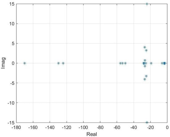
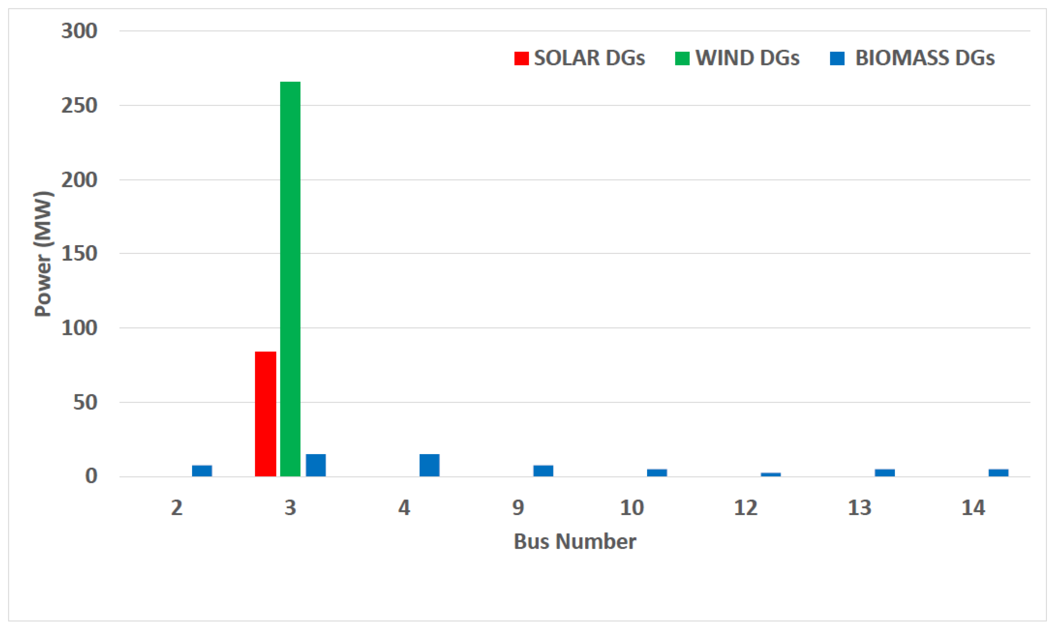
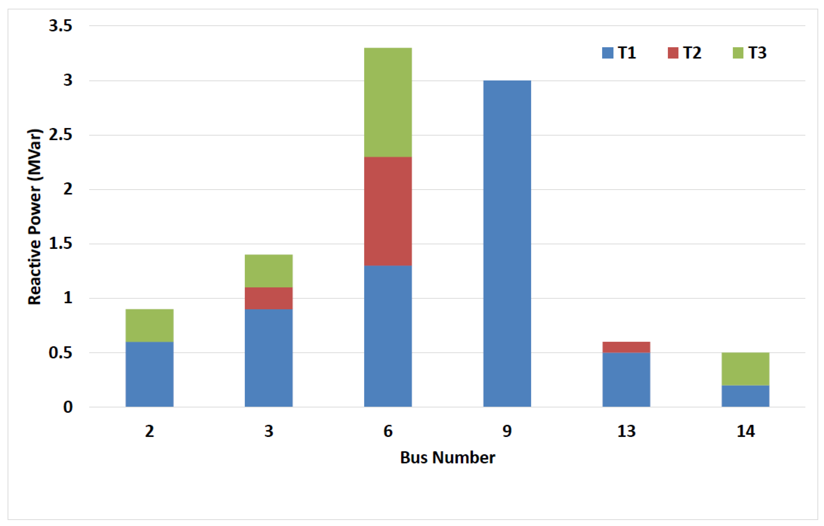
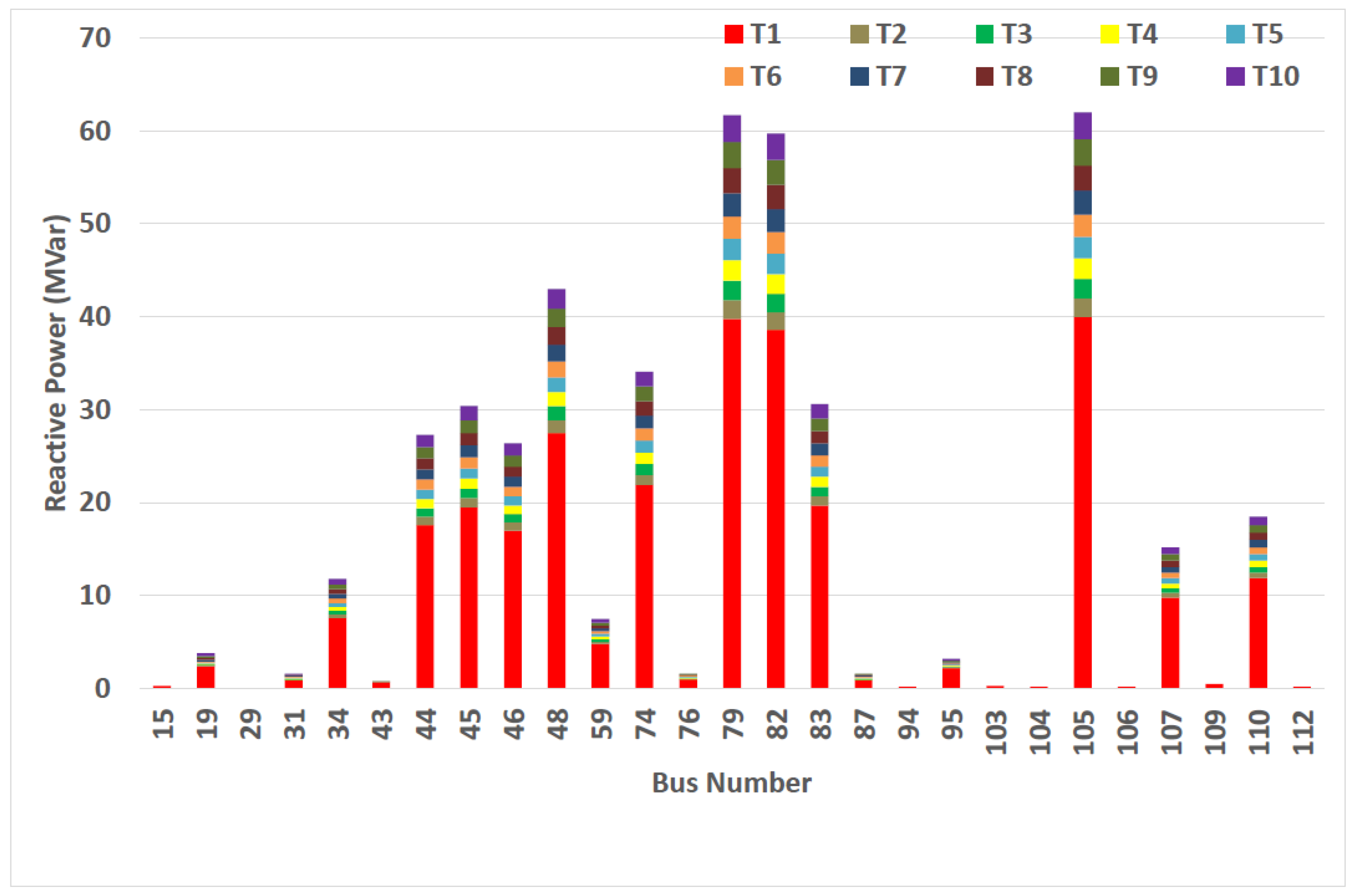
This study presented a new multi-stage distribution expansion planning mathematical model to integrate and allocate large scale hybrid renewable DGs such as solar PV, wind, and biomass (sugar cane) and capacitor banks into distribution systems optimally. The scenario based probabilistic modeling approaches, beta and Weibull distributions, were applied to model the random behavior of solar irradiance and wind speed, respectively. Biomass DG was taken as a firm generation whose capacity could be determined as and when needed. The proposed planning model decided the optimal time of integration and the numbers, sizes and location of REHDGS and reactive compensators in the distribution networks simultaneously. The main objective of this optimization work, to maximize the REHDG power generated and absorbed into the distribution networks while the long term dynamic voltage and small-signal stabilities are maintained at the required levels and a least possible NPV of the total cost, was achieved. The model was formulated as a stochastic mixed integer linear programming (MILP) problem, while the non-linear AC network was made linear with the principle of fast decoupled power flow in order to characterize the network without the loss of generality, maintain accuracy, and reduce the computational complexity. Two standard test distribution systems, the IEEE-14 bus and IEEE-118 bus, were used to validate the proposed model successfully and conduct the required assessment based on the objectives of this work. The results of both case studies indicated that integrating biomass DGs and reactive compensators with variable renewable generations (PV and wind DGs) significantly increased the amount of renewable power injected into the networks. This eventually brought about a monumental decrease in the total cost compared to meeting the load demands with the conventional generations. For the IEEE-14 bus system, 411 MW of renewable power and 9.7 MVAr of reactive power were added to the system, while the IEEE-118 bus added 1.7788 GW REHDG power and 442.7 MVAr compensators to the network. In both case studies, the dynamic voltage and small-signal stabilities were highly enhanced.
The planning model for REHDGs and capacitor banks’ integration proposed in this study demonstrated a significant improvement to the system in terms of dynamic stability enhancement, electricity and emission cost reductions, welfare, and environmental enhancement, and many other benefits accrued from it.
The formulation model proposed in this work was, therefore, a major step towards developing reliable and stable networks/grids that support the integration of large scale renewable generations.
Research in progress is focused on the application of intelligent search approaches for solving REHDGs’ allocation problem, enhancing long term dynamic stability, and estimating the economic “end effect” of the hybrid distributed generation components. Future work will be devoted to the combined investigation of harmonic losses together with the long term dynamic stability of the distribution network during the integration of large scale hybrid renewable DGs. Another future research interest is the investigation of other distributed generation technologies in relation to system power quality and dynamic stability.

Author Contributions

The mathematical formulations and programming in this work were developed within the framework of the doctorate of O.A.A. He is supervised by J.L.M. and co-supervised by Y.H. The written manuscript was extensively discussed with the supervisors.

Funding

Funding from the ESKOMPower Plant Engineering Institute (EPPEI) Specialisation Centre in Renewable Energy and Power System Studies, Stellenbosch University, South Africa, is highly acknowledged.

Acknowledgments

The authors would like to acknowledge the research support received from Tshwane University of Technology (TUT), South Africa.

Conflicts of Interest

The authors declare no conflict of interest.

References

  1. Ajeigbe, O.A.; Chowdhury, S.P.; Olwal, T.O.; Abu-Mahfouz, A.M. Harmonic control strategies of utility-scale photovoltaic inverters. Int. J. Renew. Energy Res. 2018, 8, 1354–1368. [Google Scholar]
  2. Pourbehzadi, M.; Niknam, T.; Aghaei, J.; Mokryani, G.; Shafie-khah, M.; Catalao, J.P. Optimal operation of hybrid AC/DC microgrids under uncertainty of renewable energy resources: A comprehensive review. Int. J. Electr. Power Energy Syst. 2019, 109, 139–159. [Google Scholar] [CrossRef]
  3. Slootweg, J.; Kling, W. The impact of large scale wind power generation on power system oscillations. Electr. Power Syst. Res. 2003, 67, 9–20. [Google Scholar] [CrossRef]
  4. Liu, H.; Jin, L.; Le, D.; Chowdhury, A. Impact of high penetration of solar photovoltaic generation on power system small-signal stability. In Proceedings of the 2010 IEEE International Conference on Power System Technology, Hangzhou, China, 24–28 October 2010; pp. 1–7. [Google Scholar]
  5. Pan, Y.; Liu, F.; Shen, C.; Chen, L.; Mei, S. Robust Small-Signal Stability Region of Power Systems Considering Uncertain Wind Generation. In Proceedings of the 2015 IEEE Power and Energy Society General Meeting, Denver, CO, USA, 26–30 July 2015; pp. 1–5. [Google Scholar]
  6. Shukla, D.M. Impact of Wind Turbine Generators on Stability of Power Systems. Int. J. Eng. Sci. 2017, 7, 11596–11599. [Google Scholar]
  7. Pan, Y.; Liu, F.; CHen, L.; Wang, J.; Qiu, F.; SHen, C.; Mei, S. Towards the Robust Small-Signal Stability Region of Power Systems under Perturbations Such as Uncertain and Volatile Wind Generation. IEEE Trans. Power Syst. 2018, 33, 1790–1799. [Google Scholar] [CrossRef]
  8. Ajeigbe, O.A.; Munda, J.L.; Hamam, Y. Towards Maximising the Integration of Renewable Energy Hybrid Distributed Generations for Small Signal Stability Enhancement: A Review. Int. J. Energy Res. 2019, in press. [Google Scholar]
  9. Ayodele, T.; Jimoh, A.; Munda, J.; Agee, J. Challenges of grid integration of wind power on power system grid integrity: A review. Int. J. Renew. Energy Res. 2012, 2, 618–626. [Google Scholar]
  10. Li, P.; Qi, J.; Wang, J.; Wei, H.; Bai, X.; Qiu, F. An SQP method combined with gradient sampling for small-signal stability constrained OPF. IEEE Trans. Power Syst. 2017, 32, 2372–2381. [Google Scholar] [CrossRef] [Green Version]
  11. Atwa, Y.M.; El-Saadany, E.F. Probabilistic approach for optimal allocation of wind-based distributed generation in distribution systems. IET Renew. Power Gener. 2016, 5, 79–88. [Google Scholar] [CrossRef]
  12. Murty, V.; Kumar, A. Mesh distribution system analysis in presence of distributed generation with time varying load model. Int. J. Electr. Power Energy Syst. 2018, 62, 836–854. [Google Scholar] [CrossRef]
  13. Tawfeek, T.S.; Ahmed, A.; Hasan, S. Analytical and particle swarm optimization algorithms for optimal allocation of four different distributed generation types in radial distribution networks. Energy Procedia 2018, 153, 86–94. [Google Scholar] [CrossRef]
  14. Altıntaş, O.; Okten, B.; Karsu, Ö.; Kocaman, A.S. Bi-objective optimization of a grid-connected decentralized energy system. Int. J. Energy Res. 2018, 42, 447–465. [Google Scholar] [CrossRef] [Green Version]
  15. Dicorato, M.; Forte, G.; Trovato, M. Environmental-constrained energy planning using energy-efficiency and distributed-generation facilities. Renew. Energy 2008, 33, 1297–1313. [Google Scholar] [CrossRef]
  16. Al Abri, R.; El-Saadany, E.F.; Atwa, Y.M. Optimal placement and sizing method to improve the voltage stability margin in a distribution system using distributed generation. IEEE Trans. Power Syst. 2013, 28, 326–334. [Google Scholar] [CrossRef]
  17. Salyani, P.; Salehi, J.; Gazijahani, F.S. Chance constrained simultaneous optimization of substations, feeders, renewable and non-renewable distributed generations in distribution network. Electr. Power Syst. Res. 2018, 158, 56–69. [Google Scholar] [CrossRef]
  18. Lazzeroni, P.; Repetto, M. Optimal planning of battery systems for power losses reduction in distribution grids. Electr. Power Syst. Res. 2019, 167, 94–112. [Google Scholar] [CrossRef]
  19. Sfikas, E.; Katsigiannis, Y.; Georgilakis, P. Simultaneous capacity optimization of distributed generation and storage in medium voltage microgrids. Int. J. Electr. Power Energy Syst. 2015, 67, 101–113. [Google Scholar] [CrossRef]
  20. Mahmoud, K.; Yorino, N.; Ahmed, A. Optimal distributed generation allocation in distribution systems for loss minimization. IEEE Trans. Power Syst. 2015, 31, 960–969. [Google Scholar] [CrossRef]
  21. Bagheri, A.; Monsef, H.; Lesani, H. Integrated distribution network expansion planning incorporating distributed generation considering uncertainties, reliability, and operational conditions. Int. J. Electr. Power Energy Syst. 2015, 73, 56–70. [Google Scholar] [CrossRef]
  22. Kashyap, M.; Mittal, A.; Kansal, S. Optimal Placement of Distributed Generation Using Genetic Algorithm Approach. In Proceeding of the Second International Conference on Microelectronics, Computing & Communication Systems (MCCS 2017); Springer: Singapore, 2019; pp. 587–597. [Google Scholar]
  23. Rahman, M.M.; Arefi, A.; Shafiullah, G.; Hettiwatte, S. A new approach to voltage management in unbalanced low voltage networks using demand response and OLTC considering consumer preference. Int. J. Electr. Power Energy Syst. 2018, 99, 11–27. [Google Scholar] [CrossRef]
  24. Zeb, M.Z.; Imran, K.; Janjua, A.K.; Nadeem, M.; Amin, A. Optimal Allocation and Sizing of Solar Panels Generation via Particle Swarm Optimization Algorithm. In Proceedings of the 2019 2nd IEEE International Conference on Computing, Mathematics and Engineering Technologies (iCoMET), Sukkur, Pakistan, 30–31 January 2019; pp. 1–5. [Google Scholar]
  25. Nahman, J.M.; Peric, D.M. Optimal Planning of Radial Distribution Networks by Simulated Annealing Technique. IEEE Trans. Power Syst. 2008, 23, 790–795. [Google Scholar] [CrossRef]
  26. Koziel, S.; Rojas, A.L.; Moskwa, S. Power loss reduction through distribution network reconfiguration using feasibility-preserving simulated annealing. In Proceedings of the 2018 19th IEEE International Scientific Conference on Electric Power Engineering (EPE), Brno, Czech Republic, 16–18 May 2018; pp. 1–5. [Google Scholar]
  27. Su, H. Siting and sizing of distributed generators based on improved simulated annealing particle swarm optimization. Environ. Sci. Pollut. Res. 2019, 26, 17927–17938. [Google Scholar] [CrossRef] [PubMed]
  28. Rao, R.S.; Ravindra, K.; Satish, K.; Narasimham, S. Power loss minimization in distribution system using network reconfiguration in the presence of distributed generation. IEEE Trans. Power Syst. 2013, 28, 317–325. [Google Scholar] [CrossRef]
  29. Nekooei, K.; Farsangi, M.M.; Nezamabadi-pour, H.; Lee, K.Y. An Improved Multi-Objective Harmony Search for Optimal Placement of DGs in Distribution Systems. IEEE Trans. Smart Grid 2016, 4, 557–567. [Google Scholar] [CrossRef]
  30. Abdelaziz, A.; Hegazy, Y.; El-Khattam, W.; Othman, M. Optimal allocation of stochastically dependent renewable energy based distributed generators in unbalanced distribution networks. Electr. Power Syst. Res. 2017, 119, 34–44. [Google Scholar] [CrossRef]
  31. Reyes, L.M.; Baeza, J.M. Simultaneous Optimization of Topology, Distributed Generation and Energy Storage Systems in Distribution Networks Using the MOHBB-BC Algorithm. In Proceedings of the 2018 IEEE International Conference on Automation/XXIII Congress of the Chilean Association of Automatic Control (ICA-ACCA), Concepcion, Chile, 17–19 October 2018; pp. 1–6. [Google Scholar]
  32. Othman, M.; El-Khattam, W.; Hegazy, Y.; Abdelaziz, A.Y. Optimal placement and sizing of voltage controlled distributed generators in unbalanced distribution networks using supervised firefly algorithm. Int. J. Electr. Power Energy Syst. 2016, 82, 105–113. [Google Scholar] [CrossRef]
  33. Gerez, C.; Silva, L.I.; Belati, E.A.; Sguarezi Filho, A.J.; Costa, E.C. Distribution Network Reconfiguration Using Selective Firefly Algorithm and a Load Flow Analysis Criterion for Reducing the Search Space. IEEE Access 2019, 7, 67874–67888. [Google Scholar] [CrossRef]
  34. Prabha, D.R.; Jayabarathi, T.; Umamageswari, R.; Saranya, S. Optimal location and sizing of distributed generation unit using intelligent water drop algorithm. Sustain. Energy Technol. Assess. 2015, 11, 106–113. [Google Scholar] [CrossRef]
  35. El-Ela, A.A.A.; El-Sehiemy, R.A.; Abbas, A.S. Optimal placement and sizing of distributed generation and capacitor banks in distribution systems using water cycle algorithm. IEEE Syst. J. 2018, 12, 3629–3636. [Google Scholar] [CrossRef]
  36. Munoz-Delgado, G.; Contreras, J.; Arroyo, J.M. Joint expansion planning of distributed generation and distribution networks. IEEE Trans. Power Syst. 2015, 30, 2579–2590. [Google Scholar] [CrossRef]
  37. Santos, S.F.; Fitiwi, D.Z.; Shafie-Khah, M.; Bizuayehu, A.; Catalao, J.; Gabbar, H. Optimal sizing and placement of smart grid enabling technologies for maximizing renewable integration. In Smart Energy Grid Engineering; Academic Press: Cambridge, MA, USA, 2017; pp. 47–81. [Google Scholar]
  38. Mishra, S.; Bordin, C.; Tomasgard, A.; Palu, I. A multi-agent system approach for optimal microgrid expansion planning under uncertainty. Int. J. Electr. Power Energy Syst. 2019, 109, 696–709. [Google Scholar] [CrossRef]
  39. Alturki, M.; Khodaei, A. Increasing Distribution Grid Hosting Capacity through Optimal Network Reconfiguration. In Proceedings of the 2018 IEEE North American Power Symposium (NAPS), Fargo, ND, USA, 9–11 September 2018; pp. 1–6. [Google Scholar]
  40. SASA. South African Sugar Industry Directory 2019/2020; South African Sugar Association Report 2019; SASA/Lightship Studios: Durban, South Africa, 2019; pp. 1–60. [Google Scholar]
  41. ESKOM. Effective Management of Energy Demand; ESKOM: Sandton, South Africa, 2016; pp. 1–21. [Google Scholar]
  42. Blank, L.; Tarquin, A. Engineering Economy; McGraw-Hill Science/Engineering/Math.: New York, NY, USA, 2011. [Google Scholar]
  43. Phonrattanasak, P. Optimal placement of DG using multiobjective particle swarm optimization. In Proceedings of the 2010 2nd IEEE International Conference on Mechanical and Electrical Technology (ICMET), Singapore, 10–12 September 2010; pp. 342–346. [Google Scholar]
  44. Stoot, B.; Alsac, O. Fast decoupled load flow. IEEE Trans. Power Appar. Syst. 1974, 859–869. [Google Scholar] [CrossRef]
  45. Gibbard, M.J.; Pourbeik, P.; Vowles, D.J. Small-Signal Stability, Control and Dynamic Performance of Power Systems; University of Adelaide Press: Adelaide, Australia, 2015. [Google Scholar]
  46. Amin, M.; Molinas, M. Small-signal stability assessment of power electronics based power systems: A discussion of impedance-and eigenvalue-based methods. IEEE Trans. Ind. Appl. 2017, 53, 5014–5030. [Google Scholar] [CrossRef]
  47. Shah, R.; Mithulananthan, N.; Sode-Yome, A.; Lee, K.Y. Impact of large-scale PV penetration on power system oscillatory stability. In Proceedings of the IEEE PES General Meeting, Providence, RI, USA, 25–29 July 2010; pp. 1–7. [Google Scholar]
  48. Sadamoto, T.; Chakrabortty, A.; Ishizaki, T.; Imura, J.-i. Dynamic Modeling, Stability, and Control of Power Systems with Distributed Energy Resources. arXiv 2018, arXiv:1804.04933. [Google Scholar]
  49. Rodriguez, C.; Amaratunga, G. Dynamic stability of grid-connected photovoltaic systems. In Proceedings of the IEEE Power Engineering Society General Meeting, Denver, CO, USA, 6–10 June 2004; pp. 2193–2199. [Google Scholar]
  50. Mosetlhe, T.C.; Yusuff, A.A.; Hamam, Y. Assessment of small-signal stability of power systems with wind energy conversion unit. In Proceedings of the 2017 IEEE AFRICON, Cape Town, South Africa, 18–20 September 2017; pp. 1089–1094. [Google Scholar]
  51. Condren, J.; Gedra, T.W. Expected-security-cost optimal power flow with small-signal stability constraints. IEEE Trans. Power Syst. 2006, 21, 1736–1743. [Google Scholar] [CrossRef]
  52. IRENA. Renewable Power Generation Costs in 2018; International Renewable Energy Agency: Abu Dhabi, UAE, 2019; pp. 1–88. [Google Scholar]
  53. Department of Energy. Integrated Resource Plan for Electricity 2010–2030; Integrated Resource Plan 2030; Final Report; Department of Energy, Republic of South Africa: Pretoria, South Africa, 2011; Volume 2, pp. 1–73.
  54. Azadani, E.N.; Hosseinian, S.; Divshali, P.H.; Vahidi, B. Stability constrained optimal power flow in deregulated power systems. Electr. Power Compon. Syst. 2011, 39, 713–732. [Google Scholar] [CrossRef]
  55. Zeng, B.; Zhang, J.; Yang, X.; Wang, J.; Dong, J.; Zhang, Y. Integrated planning for transition to low-carbon distribution system with renewable energy generation and demand response. IEEE Trans. Power Syst. 2014, 29, 1153–1165. [Google Scholar] [CrossRef]
  56. Al-Roomi, A.R. Power Flow Test Systems Repository; Electrical and Computer Engineering, Dalhousie University: Halifax, NS, Canada, 2015. [Google Scholar]
Figure 1. Optimal locations and sizes of PV, wind, and biomass DG power installed throughout the planning horizon.
Energies 12 04777 g001
Figure 2. Optimal capacities of reactive compensators installed throughout the planning horizon.
Energies 12 04777 g002
Figure 3. Voltage profile of the IEEE-14 bus system (base case).
Energies 12 04777 g003
Figure 4. Eigenvalues plot of IEEE-14 bus system (base case).
Energies 12 04777 g004
Figure 5. Eigenvalue plot of the IEEE-14 bus system with REDGs.
Energies 12 04777 g005
Figure 6. Optimal locations and sizes of PV, wind, and biomass DG power installed throughout the planning horizon.
Energies 12 04777 g006
Figure 7. Optimal capacities of reactive compensators installed throughout the planning horizon.
Energies 12 04777 g007
Figure 8. Voltage profile of the IEEE-118 bus system (base case).
Energies 12 04777 g008
Figure 9. Eigenvalue plot of the IEEE-118 bus system (base case).
Energies 12 04777 g009
Figure 10. Eigenvalue plot of the IEEE-118 bus system with REDGs.
Energies 12 04777 g010
Table 1. Optimal investment solution of renewable energy hybrid distributed generations (REHDGs) for distribution system planning.
TypeBusStages TypeBusStages
T1T2T3 T1T2T3
x g , i , t x g , i , t
Biomass2333 Biomass9233
Solar3172535 Biomass10222
Wind37494115 Biomass12111
Biomass3666 Biomass13222
Biomass4566 Biomass14112
Table 2. Optimal investment solution of capacitor banks for distribution system planning.
TypeStages TypeStages
T1T2T3 T1T2T3
x c b , i , t x c b , i , t
2669 9303030
391114 13566
6132333 14225
Table 3. IEEE-14 bus system: Comparison of critical modes with their oscillatory frequencies and damping ratio.
Oscillatory ModesDamping Ratio ( % ) Oscillatory Frequencies (Hz)
Base Case 1.52 ± 20.26 i 3.773.17
With REHDGs 24.93 ± 15.00 i 85.682.39
Table 4. Optimal investment solution of REHDGs for distribution system planning.
Type Stages
T1T2T3T4T5T6T7T8T9T10
x g , i , t
Biomass17777777777
Biomass32222222233
Biomass43444444444
Biomass65555555555
Biomass72222222222
Biomass102222222222
Biomass116666666666
Biomass133334444444
Biomass142222222222
Biomass157777777777
Biomass164444444444
Biomass185667777777
Biomass202222222222
Biomass221111111111
Biomass231111111111
Biomass252222222222
Biomass276666666666
Biomass292222233333
Biomass313333333333
Biomass322235555555
Biomass333333333333
Biomass344444455555
Biomass352222222233
Biomass363333333333
Biomass394444444444
Biomass405556666666
Biomass412222233333
Biomass427777777777
Biomass431111111111
Biomass453344444444
Biomass462222222223
Biomass474444444444
Biomass481111111111
Biomass495677777788
Biomass502222222222
Biomass523333333333
Biomass532222222222
Biomass547777777777
Biomass554444444444
Biomass568888888889
Biomass582222233333
Solar596471788694103113123123123
Wind59117131131131131131131131131131
Biomass598888899999
Biomass607777777777
Biomass625555555555
Biomass634444444444
Biomass673333333444
Biomass705566677778
Biomass721111111111
Biomass732222222222
Biomass744555555556
Biomass764444446667
Biomass776677777777
Biomass792222222222
Biomass808888889999
Biomass853333333333
Biomass862222222222
Biomass883333333445
Biomass893333333333
Solar90 1123
Wind90 1428446281102118128
Biomass908888889999
Biomass912222222222
Biomass936666667777
Biomass952222222455
Biomass964444666666
Biomass984444555566
Biomass994555666666
Biomass1013333444444
Biomass1031111111345
Biomass1053444444444
Biomass1074445555555
Biomass1091111222222
Biomass1112222222222
Biomass1125555555666
Biomass1131111111111
Biomass1152222222233
Biomass1168888889999
Biomass1173333333333
Biomass1184455555555
Table 5. Optimal investment solution of capacitor banks for distribution system planning.
BusStages
T1T2T3T4T5T6T7T8T9T10
x c b , i , t
153333333333
1924252627282931333538
31991011121314151516
34768084889297102107112118
437777777788
44176185194204214225236248260273
45195205215226237249262275289304
46170179188197207217228239251264
48275289304319335352370389409430
5948505356596265687175
74219230242254267280294309325341
7610101112131414151616
79398418439461484508533560588617
82386405425446468491516542569597
83197207217228239251264277291306
87991011121314151616
942222222222
9522232425262727283032
1033333333333
1042222222222
105400420441463486510536563591620
1062222222222
10798103108113119125131138145152
1095555555555
110119125131138145152160168176185
1122222222222
Annual Total2857299831483305346936413823401542164427
Table 6. IEEE-118 bus system: Optimized cost information for the ten year planning horizon ( × 10 9 $ ) .
Cost FunctionStagesOverall Total
T1T2T3T4T5T6T7T8T9T10
Investment151.397.577.958.358.769.209.6610.1410.6511.18234.85
Maintenance3.023.183.343.513.683.864.064.264.474.7138.09
Energy3.423.593.763.954.154.354.574.795.045.3042.92
Emission18.7019.5520.5221.5522.6423.7624.9526.2127.5128.90234.29
Annual Total176.5333.8935.5737.3639.2341.1743.2445.4047.6750.07
C T N P V 550.15
Table 7. IEEE-118 bus system: Comparison of critical modes with their damping ratio and oscillatory frequencies.
Oscillatory ModesDamping Ratio ( % ) Oscillatory Frequencies (Hz)
Base Case 0.02 ± 20.57 i 0.093.27
With REHDGs 28.92 ± 4.23 i 98.940.67

