1. Introduction
Solar glare is an optical phenomenon that affects people whenever the angle between Sun rays and line of sight falls within their field of view (FOV). The smaller the angle the more intense the effect of glare, which can even cause temporary blindness. If people are driving a vehicle, since they have to keep their eyes on the road, the effect of solar glare occurs normally at low Sun elevation angles and can be dangerous, hindering the perception of other cars, obstacles or persons on the road. Solar glare on roads is often the cause of traffic jams [
1] and even accidents [
2,
3,
4]. Traffic jams or simply the speed reduction caused by solar glare has negative impacts on road transportation companies, affecting the economy and urban mobility in general [
5]. This is a relevant issue, especially in higher latitudes where the periods during which the Sun is low in the sky are longer, potentiating glare, but also in countries of middle latitudes where clear sky conditions are frequent throughout the year. In the case of accidents, since it is an involuntary incapacitating factor for the driver, it is important to determine whether solar glare was present, eventually attenuating the guilt of the drivers involved. Confirmation of the existence of solar glare in these situations is especially relevant for auto insurance companies in post-accident cases resolution. In order to be provided with rigorous information in these situations, a high-resolution assessment of the road network is required for solar glare determination on the site and for the exact time of the accident. Astronomical observatories are often asked for technical assessments in this matter to be presented in court [
6].
In a non-overcast sky, solar glare happens whenever the solar incidence angle is within the FOV of the driver and the vehicle is not in shadow cast by terrain relief, isolated clouds, neighbouring buildings or trees, which cause a temporary failure of Sun visibility. In urban areas, shadow cast by trees, buildings or other constructions is therefore an important factor, especially at times when most glare situations occur, since shadows are longer by lower Sun elevations. This means that in these areas, not only the road network but also the influence of their immediate neighbourhood, must be considered. Due to high relief amplitude in the urban area, the shadows cast by far terrain features, like high mountains, should also be integrated [
7]. Also, the type of vehicle is relevant, since the height of the driver’s eyes is different in a light or in a heavy vehicle. A wall along the street can cast shadows on the pavement and the driver can still be dazzled when his/her eyes are above the shadow. Light and heavy vehicle cases have to be studied separately. Some studies also indicate that age, visual health and the intensity of Sun glare are some of the critical factors that strongly influence a driver’s performance [
8,
9].
The solar incidence angle is the angle between a Sun ray (from the driver’s eyes to the Sun) and the line of sight of the driver that can be considered as looking straight forward in the same direction as the road axis. Considering a winding road for better understanding, this angle, for a certain position of the Sun (i.e., for a certain day and time), changes along the road according to the azimuth and slope of the actual road section axis. On the other hand, for the same position on the road, the incidence angle changes throughout the day and the year with the position of the Sun in the sky. Some sections of the road are never affected by glare, others are affected during one period of the day, others during two distinct periods, one in each driving direction. Slope and azimuth are different in each driving direction of the same road section, so each direction must be studied separately.
Some authors approach solar glare with different objectives and results. Most studies in this domain use a digital terrain model (DTM) and a road network map to predict the presence of solar glare [
2,
10]. Richter and Löwner showed [
11] that it was possible to map solar glare in a highway network with a time resolution of 15 min, using Open Street Map data as geometric input. A glare map, where highway sections are classified according to the glare risk (no glare, from the front, from the front despite the Sun visor, from the sides, from the rear, etc.), was produced for every time step. A time series of glare maps constitutes the result. However, the authors do not explain how they dealt with both driving directions on the same section. The glare map is not clear about the driving direction on the highway that was analysed for glare along the network. Furthermore, slope is not taken into account, neither are shadows. The authors point out the intensive calculations and long accesses to the databank which are also a bottleneck for other approaches. Khumalo and Vanderschuren [
12] used the
Hillshade function of ESRI ArcGIS (Environmental Systems Research Institute, Redlands, CA, USA) [
13] to study solar glare in the streets of Cape Town (South Africa). The study was limited to the solstice and equinox days and neither street slope nor building shadows were considered in the results. Jurado-Piña and Mayora [
4] developed a methodology based on cylindrical charts to determine the maximum tolerable solar glare at a specific angular distance between a driver’s line of sight and the Sun (incidence angle), considering the characteristics of the surrounding environment. According to this study, that angular distance is 19° for a 40-year-old driver and 25° for a 60-year-old driver. Aune [
10] presented a method for calculating the presence of solar glare on roads and developed a plug-in for QGIS (QuantumGIS, Free and Open Source Software for Geographic Information Systems) [
14] to visualize solar glare data. By using road and terrain data, the method calculates whether roads have solar glare or not at any given time. Roads are identified by a set of point features with east, north and elevation coordinates. The used DTM presents a spatial resolution of 10 m. Calculations are performed for the whole year on all road segments, only for rush hours (7–9 a.m. and 3–5 p.m.) with a time resolution of 5 min. The “Sun Glare Detection System—SGDS” is developed in 4 main steps. After identifying the road segment of interest, the Sun’s position relative to each of the road points is calculated. An occlusion test is done at each road point, analysing the surrounding terrain and considering limits for the horizontal and vertical angular aperture for glare detection. Slope and driving direction are calculated based on the road points and the DTM. The study of Aune [
10] is strongly conditioned by two main and relevant aspects—one relates to the positional and vertical quality of the input data and the other, more methodological, concerns the analysis of the surrounding terrain and the corresponding occlusions. The spatial resolution of the data (10 m) leads to inaccurate calculations of driving directions, as well as the poor vertical accuracy of the altimetric data used (± 2 m to 3 m standard deviation [
15]) leads to inaccurate calculation of slopes, with direct and obvious consequences in identifying the presence of glare. Apart from this aspect, during occlusion analysis only terrain elevation is considered, neglecting all urban objects that may contribute to the reduction of solar glare, like trees or tall buildings that cast shadows and reduce or eliminate the glare effect. In addition, the author is rather vague about the driving direction as the input parameter for calculation. It is well known that driving orientation determines whether or not the driver is dazzled, so it is imperative to present the results in both driving directions on the same road segment, which was not done in the study of Aune [
10]. A very different approach is presented by Li et al. [
16] where a series of historic panorama images from Google Street View were used to evaluate solar glare in discrete positions (40 m apart) along the roads of a town, considering the existing sky obstructions in each point and the projected Sun positions on a cylindrical surface centred on the driver’s position (assuming the driver is in the position of the Google Street View camera). In this approach, deep convolutional neural network algorithms were used to classify the pixels of each panorama picture in order to identify the sky pixels. If the projected position of the Sun falls on a sky pixel of the panoramic image, there is Sun glare. Not only the presence but also the duration of glare was mapped and divided in two classes—less than 100 and more than 100 min. The resulting glare maps are not clear about the driven direction and the authors do not mention how they got glare duration in each point.
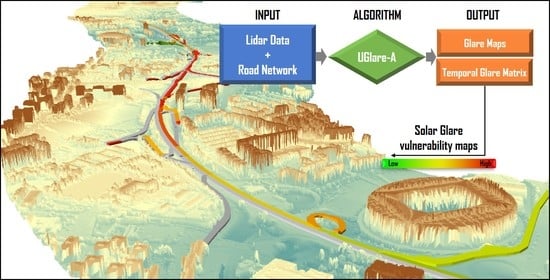
The present work shows an innovative approach to producing high resolution solar glare maps in urban areas. An algorithm is developed for generating the terrain and buildings’ shadows and to determine the presence of glare conditions. The road network is analysed in the form of oriented and properly georeferenced graph where each edge corresponds to a road section. Each driving direction, of the same edge, is considered separately for calculations. Each type of vehicle, light or heavy, is also evaluated separately. For each road section, a map with glare location is produced for each epoch in one year. In addition to the maps and simultaneously to its calculation, a temporal binary matrix is created for each section, showing when, along the year, glare happens in the street segment in each driving direction.
With these results, vulnerability to solar glare can be estimated considering both a cloudless sky (
Section 3.3) and a typical overcast sky (
Section 3.4).
2. Data and Methodology
Although the methodology presented below can be applied everywhere, it was tested for a concrete area (2ª Circular road) in Lisbon, Portugal (
Figure 1). The 2ª Circular road, besides presenting a favourable orientation to the occurrence of solar dazzling for those who circulate on it, is classified as the worst road in the city of Lisbon in terms of road accidents, with 838 casualties, 12 registered deaths, 25 seriously injured and more than 1000 minor injured in a six-year period (2010–2016) [
17].
2.1. Input Data
Road polylines and airborne LiDAR data are the geometric data basis for the present methodology. Road polylines were available as a shapefile provided by the Municipality of Lisbon [
18], containing a set of specific attributes such as the name and level of road hierarchy and some of its geometric attributes (e.g., length). Height data were available from an airborne LiDAR survey of Lisbon executed in 2016 in the frame of the PVCITY project [
19]. Data were obtained with a density of 12 points/m
2 and delivered in LAS format. A DSM (Digital Surface Model) and a DTM were generated from the LAS data, in a raster format with a resolution of 1m. Nominal accuracy of the data is given as ± 0.15 m in XY and ± 0.08 m in Z [
20]. Astronomical equations are used for calculating Sun/shadow orientation as well as Sun azimuth and elevation.
2.2. Data Pre-Processing
Data preparation before glare calculation consisted of three main parts which are graphically depicted in the workflow presented in
Figure 2. The figures that are part of the workflow show the pre-processing results for a specific road section of the 2ª Circular in order to exemplify the procedure that was automated for the treatment of all sections of this studied road. Pre-processing operations were executed in ArcMap (10.6, Environmental Systems Research Institute, Redlands, CA, United States of America) [
13].
Phase 1—in the first part, a set of topological corrections was applied to the road network in order to generate an oriented graph. Polylines were first divided into edges and nodes. Each road section (main edge) of the network consists of an edge, a start node, where the movement begins, and an end node where the movement ends. The start and end nodes correspond to points of intersection with other roads and all nodes were numbered sequentially. Road sections were identified by the limiting nodes of the respective edges, whereas, for all edges that could be driven both ways, two road sections were generated—Section AB and Section BA, A and B being the limiting nodes of the edge.
Figure 3 shows an example for a route that is composed of a sequence of directed road sections designated by
start node ID–end node ID. For example, Route M–N includes sections 1–2, 2–4, 4–5, 5–7 and 7–9, while Route O–P includes sections 6–5, 5–4 and 4–11 for instance. The edge between nodes 4 and 5 appears in both routes but in distinct driving directions, constituting distinct sections.
Phase 2—in the second part, each road section was divided into 5 m long sub-sections (secondary edges) along the axis, each one constituting the smallest study unit of the road. This length was chosen to represent the mean length of a European car. This was necessary because most road sections do not maintain azimuth and slope all along the section. The azimuth and slope of each 5 m sub-section were calculated for both driving directions. To simplify the study, the azimuth and slope of each 5 m sub-section were considered constant along the sub-section. Due to the dimensions of a car on the road, this was considered accurate enough. Though heavy vehicles are longer, the resolution was maintained. After this step, four grid tiles were generated, dimensioned by the minimum bounding box (MBB) of each road section (main edge)—two grid tiles containing a buffer of 15 m, to each side of the road axis, filled with the slope value, of each sub-section, one per each driving direction; the other two grid tiles were similar but containing the azimuth values also for both driving directions.
Phase 3—finally, in order to take the road’s neighbourhood into account, two new grid tiles were generated; one grid tile per road section (main edge). Each grid tile contains the following—a buffer of 15 m to each side of the road axis filled with the DTM values added by the driver eyes height (for a light vehicle: 1.08 m; for a heavy vehicle: 2.33 m); a strip of 50 m on both sides of these buffer limits (a distance of 65 m off the road axis) filled with the DSM values. A minimum bounding box (MBB) around this buffer limits the tile. The tiles were not disjunct since each node was the origin of several road sections. The width of the central buffer should depend on the real width of the street, which should be an attribute of the polylines. The feature layer corresponding to the road network used did not have this attribute attached, so a mean width was considered for the central buffer (15 m). This methodology for creating input data for the algorithm that detects glare situations was developed, having in mind the reduction of the computation volume to a minimum. Small tiles are prepared instead of taking the whole area covered by the network and by the DTM/DSM.
Finally, at the end of data preparation, six final grid tiles per MBB are provided—two grids (on both directions of the same road section) containing slope values of each 5 m sub-section within the 15 m buffer; two grids (on both directions of the same road section) containing road azimuth values of each 5 m sub-section within the 15 m buffer; one grid containing DTM values plus 1.08 m (for a light vehicle) and another grid containing DTM values plus 2.33 m (for a heavy vehicle), in the 15 m buffer, both being grids filled with DSM values in the buffer zone between 15 m and 65 m distance to the road axis.
2.3. The Glare Algorithm: UGlare-A
The Urban Glare Algorithm (UGlare-A) for determining the presence of solar glare in road sections and sub-sections was developed in Matlab (2017, Mathworks, Natick, MA, USA) [
21]. It runs for one year, with selectable time steps (e.g., every hour, every 30 min, every 5 min), and takes as input the directories containing the grid tiles produced before, one directory per section with complete tile for heavy vehicles, complete tile for light vehicles, azimuth tile and slope tile for each drivable section of the network. The algorithm consists mainly of five parts and runs automatically for all sets of tiles. After the computation, results are organized in a ‘queryable’ way, so that they can be picked up for a chosen route (
Figure 4).
In the first part, the Sun’s position is determined for all epochs of a day, and a simple check is done whether glare is possible according to Sun positions, azimuth and slope of the road section. If the answer is positive, for each epoch a shadow map for the actual section is generated, taking into account the neighbourhood (buildings, trees, terrain) depicted by the DSM (second part). On the road area, shadows are calculated for the height of the driver’s eyes since the surface here is equal to the DTM plus driver’s eyes’ height. In the third part, Sun azimuth and elevation are checked against glare conditions limits for all pixels which are not in shadow and belong to the road area (i.e., within the central 15 m buffer of the axis), For this, the respective sub-section slope and azimuth are considered which are picked up from the section slope and azimuth maps. A glare map for that day and epoch is generated. A temporal glare matrix is built for each section indicating at what times glare happens in the section along the year. This also indicates how many glare maps there are and the respective filename can be derived from the matrix element indexes as will be explained in
Section 2.3.5.
2.3.1. Sun Position
The apparent position of the Sun in the sky is described by its azimuth and elevation. These are local horizontal Sun coordinates, that means the reference plane is the local horizon, changing, therefore, from place to place. Solar azimuth and elevation depend on local latitude and longitude, as well as on Sun declination and Sun hour angle. Declination and right ascension are the absolute coordinates of the Sun relative to the celestial sphere, the hour angle being the complement to 24 h of the right ascension. Sun declination does not depend on the latitude nor on the longitude, but it depends on the day of the year since it changes throughout the year. In UGlare-A, every astronomical calculation is done for the middle point of the road section tile and for the set time interval. Since the biggest section tile dimension in the studied area is about 700 m, the followed approach is accurate enough. If the algorithm would be applied to a road network with much longer edges, these would have to be first subdivided in smaller segments so that astronomical calculations for the middle point would be valid for the whole tile.
First, the cartographic rectangular coordinates (X, Y) of the middle point are transformed in geodetic coordinates (latitude and longitude) over the ellipsoid. For the actual data, grid tiles were projected in the cartographic coordinate system EPSG 3763: ETRS89-PT-TM06 and were transformed to the geodetic coordinate system ETRS89 on the GRS 80 ellipsoid. Then, a table was built with the times of sunrise and sunset for the location of the middle point for every day of the year. Further, a second table was built with Sun declination, Sun hour angle, Sun azimuth and Sun elevation for every epoch, according to the set time interval, and for the location of the middle point of the road section tile. Equations (1)–(14) were used. While Equation (1) is a Fourier series development for the Sun declination which was presented in Reference [
22] and is more precise than usual formulas which consider the declination constant throughout the day, all other equations can be found in Astronomical Almanachs [
23]. Nomenclature for the equations is as follows:
Equation (1): δS—Sun declination; D—day and decimal part of the day, counting from January the 1st at 00h00.
Equations (2)–(6): t—time of the day (epoch) in hours and decimal part of an hour since midnight; EoT—equation of time; lon—longitude of the central point of the tile; hAngle—Sun hour angle.
Equations (7)–(11): elvS—Sun elevation; zenS—zenith angle of the Sun; lat—latitude of the central point of the tile; R—mean Earth radius; Dst—mean Earth-Sun distance; refAtm—atmospheric refraction correction. The latter depends from the temperature T and atmospheric pressure Pa. In UGlare-A, mean values for each month were considered in the refraction correction equation.
Equations (12)–(14): azS—Sun azimuth; mod [a/b] stays for the remainder of the integer division.
Sun elevation, elvS, and Sun azimuth, azS, are input values for the shadow algorithm and for the computation of the Sun incidence angle, if needed.
2.3.2. First Glare Test
For each tile, the road azimuth map is taken for a first glare test. To recall, this map is a raster representation of the central buffer (15 m) of the road axis, the values of which are the azimuth of the 5 m long subsections along the road, respective to the driving direction. This test consists of the following—for each day, the Sun azimuth values between sunrise and sunset were analysed. They are read from the table mentioned in
Section 2.3.1. and the minimum and maximum values were determined. A value for the driver’s horizontal Field of View (FOVxy) was defined. Although not unanimous throughout literature, a FOVxy of 120 degrees was considered, based on the value for human binocular vision presented by several authors [
24]. To simplify, the driver was considered to look straight forward along a line with the local road azimuth and the FOVxy to be symmetrical to both sides of this line, 60° wide on each side. For the vertical Field of View (FOVz), it was considered that the driver’s line of sight has the local slope of the road and that half the FOVz is an angle of 55 degrees above this line (on a vertical plane), a mean value of those found in the literature [
25,
26]. For simplicity, FOVz was considered symmetrical relative to the line of sight. Then, limits were set for the road azimuths for possible glare according to the condition (5).
In case some pixels of the tile fulfil this condition, a similar test was made for the road slope map substituting Sun azimuth by Sun elevation and FOVxy by FOVz in condition (15). Only the tiles that fulfil both conditions were further investigated. Tiles that did not fulfil the conditions in any pixel were considered not to be affected by the solar glare phenomenon during the day in question and the search continued for the next day.
2.3.3. Shadows
The shadow algorithm used in UGlare-A is adapted from the one presented in Reference [
27]. It runs only for the epochs between sunrise and sunset and only for the sections that passed the test referred to in
Section 2.3.2. The shadow was calculated in profiles of the tile with an orientation equal to the Sun azimuth plus 180 degrees. Each profile contains the values of the DTM plus driver eyes’ height on the road area (15 m buffer of the axis) and the DSM values on each side of the road (50 m strip on each side). The height of the driver’s eyes was set to 1.08 m for light vehicles and 2.33 m for heavy vehicles, according to the AASHTO (American Association of State Highway and Transportation Offcials) [
28]. The shadow for light vehicles and heavy vehicles is calculated separately using the respective tiles. This way, shadows on the pavement cast by low obstacles near the road were not considered, since the driver can look over these obstacles and get dazzled by the Sun.
The algorithm considers a spatial ray with an inclination equals the Sun elevation that is propagated from the height and position of the first pixel along each profile, losing height as it runs, proportionally to the travelled way and the tangent of the Sun elevation angle (
Figure 5, bottom right). All pixels of the profile below the ray are in shadow (cast by relief, buildings, or trees). Every time the ray reaches a point of the profile higher than the actual ray height at that location, the ray assumes the height of the reached point (which is not in shadow) and continues to run the profile as before to detect new points of the profile, which are in shadow. At the end of the profile, pixels in shadow were transferred with their XY coordinates to a map, with the same dimensions as the original tile, that is, a successively filled profile by profile with black or white pixels. The juxtaposition of the transferred XY-projected profiles builds a binary shadow map (0 = shadow, 1 = no shadow) once every profile with the same direction having been run.
2.3.4. Detection of Glare
Glare happens whenever the direction of the Sun rays makes an angle to the driving direction that is smaller than the driver’s angular FOV. Since we considered a solid angle for the driver’s FOV limited by horizontal and vertical angles (
Figure 6), and the driver’s line of sight is aligned with the road axis sharing its azimuth and slope, the conditions favourable for glare are the following—the absolute difference between Sun azimuth and road azimuth must be less than half FOVxy and simultaneously the absolute difference between Sun elevation and road slope must be less than half FOVz.
Shadow maps, for light and heavy vehicles, were the base for the fine glare test, together with road azimuth and slope maps. Only pixels that were not in shadow were checked for glare, and a binary glare map was produced for each tile and for each epoch (1 = glare in the pixel location, 0 = no glare in the pixel location). Maps with only no glare pixels were not saved. Glare maps are grids (raster) with a resolution of 1m that can be seen as binary images.
2.3.5. Temporal Matrix
The temporal matrix was created once for each drivable section and was a binary one (0 = no glare in the section, 1 = glare within the section). It has 365 columns, one for each day of the year, and 24 times n rows, n being the number of parts of an hour corresponding to the set time interval (e.g., for an interval of 15 min = 1/4 h, n = 4). Only matrices which were not null were saved, together with the respective glare maps, so that time and location of glare along a section were documented. At the same time, a rapid search for glare existence can be made only at the matrix level, avoiding having to process the raster images all the time. Each matrix element different to zero corresponds to one glare map, the file name of which can be easily derived from the matrix indexes of the element (column = day, line = epoch, filename: ‘glaremap_day_epoch’). Vulnerability analysis from the point of view of the time periods when glare happens in a section can also be made using these matrices. They can be visualized as images and rapidly show if a section is vulnerable to glare only in the morning or only in the afternoon or in both periods, how long and when in the year.
3. Results
The results of UGlare-A can be explored in several ways. Some examples are given in the following.
3.1. Glare in the Network
Although glare maps are produced for each section and time, it does not make much sense to visualize a whole street network with the respective raster glare maps for a specific epoch. Both driving directions would superimpose and not much information would come out. If a whole network should be studied at a specific epoch, the information in the glare maps should be transferred to the road axis in a vector map, and this one should be represented as a double line, one line for each direction, whenever drivable in both directions. For a study along a time period, a series of vector maps with glare information over double road axis should be prepared and watched dynamically (video animation).
3.2. Glare along a Route
The interpretation of results in the format suggested in
Section 3.1. is, nevertheless, difficult. To determine which street location is more vulnerable to glare, at what time and in which driving direction, when a whole double lined network blinks in the screen, is not easy. It makes more sense to analyze routes instead of the whole network. Is this route more or less vulnerable to solar glare than the other, near sunrise or sunset? A route has only one driving direction and glare can be represented directly over the road axis. For a period, again a dynamic representation had to be prepared to reflect the spatial temporal character of the variable solar glare. The glare analysis along a route is also adequate for implementation in car navigation systems.
3.3. Vulnerability to Solar Glare
The vulnerability of a road section to solar glare, obtained from the number of time intervals in which glare exists, can be calculated at matrix level. Since all temporal matrices have the same dimension, distinct road sections can be easily compared. Rush hour periods can also be analyzed comparatively since they correspond to the same lines in all matrices.
Figure 7,
Figure 8 and
Figure 9 show some examples for light vehicles.
The temporal matrix in
Figure 7 reveals that the road Section 23–22 is prone to solar glare twice a day along the whole year. This is due to the strong variation in azimuth and slope along the road. The section is a circular motorway exit. Glare is particularly dangerous in this kind of sections since it appears suddenly as the driver turns from the highway to another road, which is normally at a different level. Of course, the places in the section where morning and evening glare appear are not the same. The temporal matrix refers to the whole section.
Figure 8 shows the glare behavior along the year in both driving directions—51–53 and 53–51. It is clear that morning glare periods begin later in the winter than in the summer and the opposite happens for the evening glare. Since the sections’ orientations are nearly W–E and E–W, the daily glare duration is almost constant along the year.
As for the sections shown in
Figure 9, presenting nearly S–N and N–S orientations, the temporal matrix shows that section 12–15 only has glare (morning glare) in the summer while section 15–12 has glare along the whole year, longer in the winter, and shorter during summer.
This temporal analysis can be made for every road section on base of the temporal matrices.
The vulnerability of a road section can be calculated by the number of days per year that solar glare exists at a specific epoch. Because solar glare represents an added danger factor at rush hours,
Figure 10 shows the results for morning and evening rush hours for a part of the studied road network. The road sections are classified by the number of days in the year that solar glare happens at each considered epoch, assuming a non-overcast sky. Both driving directions are represented wherever the road is drivable both ways. In Lisbon, there is right-hand traffic.
As for the local vulnerability in one road section, this can be studied on the basis of the glare maps. A sum of the grids yields a map with the number of time intervals in which glare appears in each pixel along a selectable period—an hour, a month, a season, a year.
Figure 11 shows an example for the road sections from node 23 to node 36, in the indicated driving direction. The influence of the nearby buildings and trees is noticeable in the blueish areas. In the winter and autumn maps, there are even several positions without glare during the whole season (represented by transparent pixels). This proves the efficiency of the shadow algorithm, fundamental to glare identification in urban areas.
This kind of analysis reveals road areas that are affected by glare in all seasons, as well as areas that are seldom affected. By identifying the areas with the most frequent glare occurrence throughout the year, traffic managers can use this type of result to plan with better spatial and temporal accuracy the information to be provided to drivers, for example, through variable message boards at specific locations and showing the message during a specific time period.
Being a georeferenced product, glare maps like those shown in
Figure 11, when calculated for a certain day and time, allow determination of the existence or absence of glare at a point located with a high spatial accuracy (1 m). This is an important tool for clarifying accidents.
3.4. Vulnerability to Solar Glare Considering Weather Conditions
The results shown in
Section 3.3 assume, as referred to in the text, a non-overcast sky during the whole year, which can be interpreted as the potential vulnerability to solar glare or as the worst-case scenario. To clarify whether an accident was partially caused by solar glare or to display appropriate information in variable message boards, the local weather conditions at the time of the accident or on road segments susceptible to glare, must be considered, since, with an overcast sky, there is no solar glare.
Unlike in the case of the Sun, there is still no way to predict the position of clouds in the sky at a particular epoch. However, for a more realistic modeling of solar glare vulnerability, typical weather conditions for the region based on climatic observations should be considered, which can tell us the percentage of time the sky is typically overcast. Clearly, this information has to be interpreted with care, since it does not precisely establish in which periods of the day the sky was overcast. An overcast sky can last a whole day, be only in the morning or only in the late afternoon hours. A 50% probability of overcast sky in a month does not tell us whether the sky was overcast every morning or every second day. In statistical terms, however, to calculate vulnerability, considering cloud coverage is closer to reality than considering a cloudless sky along the whole year.
Road vulnerability to solar glare considering typical weather conditions in Lisbon was calculated and is shown in
Figure 12 for the rush hours that presented higher vulnerability (see
Figure 10). Cloud coverage data were retrieved from Weather Spark [
29], a site that reports typical climate data for any spot on Earth in monthly, daily and hourly graphics. According to the authors of the site, the data are based on a statistical analysis of historical hourly reports and model reconstructions from 1 January 1980 to 31 December 2016, a period of 37 years. The meteorological model used is the MERRA-2 (Modern Era Retrospective analysis for Research and Applications, Version 2) from NASA (National Aeronautics and Space Administration) [
30]. Cloud coverage is classified in five classes—overcast, almost overcast, partially overcast, almost clear, clear. Only the percentage for overcast sky was considered, since this is the condition of absence of glare everywhere (
Table 1).
Vulnerability results obtained as described in
Section 3.3. were multiplied by a ‘clear sky factor’ equal to 1 minus percentage of overcast, depending on the month of each epoch, yielding a more probable vulnerability value under typical weather conditions. As depicted in
Figure 12, the resulting vulnerability decreases when compared to the previous model, meaning that, typically, each road section is subjected to solar glare fewer days in the year at the indicated time.
4. Discussion and Conclusions
The presented methodology to produce high resolution solar glare maps was shown to be efficient for solar glare vulnerability studies in urban areas. Urban landscape specificities are included in the calculation by using DSM information of the road neighbourhood obtained from an airborne LiDAR survey with 12 point/m2 density. Driver eyes’ height is also considered along the road, using a height surface over the road that is equal to the DTM plus driver eyes’ height (1.08 for light and 2.33 for heavy vehicles). This way, shadows on the road, cast from nearby buildings and trees, are calculated for the driver eyes’ height.
Both the methodology for data pre-processing in a GIS environment and the UGlare-A algorithm run automatically for a road network. Results of the process are for each road section (oriented graph edge), one temporal matrix and several glare maps, one for each day and epoch of the year in which glare happens in the section. The temporal matrix shows ‘when’ and the glare maps show ‘where.’ Glare maps have a spatial resolution of 1 m.
As conditionings of the application of the presented methodology, the topological quality of the road network, including attributes and the spatial resolution and geometric quality of the DSM/DTM, can be pointed out. The extension and density of the urban road network determine the volume of calculation and consequently the amount of output files. Nevertheless, once completed, the recalculation is only necessary if the network geometry or the urban height surface (DSM) changes. Additionally, an integrated solution for pre-processing and glare calculation could be more operative. There are no restrictions in the methodology that prevent it being applied to more extensive areas. Only the amount of data and the required computing time can be limitative if enough resources are not available. LiDAR data, although becoming more and more common, are still an expensive factor and are not available everywhere. Nevertheless, point clouds produced from aerial photography with modern photogrammetry and computer vision automatic operators can also be used for producing the needed height surface. Aerial photography coverages are more common than LiDAR data, since they are used everywhere for mapping.
The way results are organized is suitable for rapid access as an input for result exploring algorithms. In this work, some examples of result exploring are shown, focused on accessing the vulnerability to solar glare. Temporal matrix analysis, for instance, allows a rapid perception of the glare periods on a road section along a year. It also serves as an index to existing glare maps in order to optimise calculation time. Temporal matrices are also the basis for a classification of the network edges according to the number of days in the year that each edge suffers solar glare at a specific epoch. Applied to rush hour periods, this analysis, as shown in
Figure 10, can be very useful. The representation of the road network with both driving directions, wherever they exist, and differentiated information for each direction, as in
Figure 10, is shown to be an intuitive information transmission means, never found before in solar glare studies. A driver can identify the driving direction he wants to follow and see if there is glare danger or not at a specific travel time (interval).
Vulnerability to solar glare was calculated as the sum of times glare happens in a position or in a road section during a certain time interval. It was calculated, on the one hand, considering a cloudless sky, which configures a worst-case scenario relevant for signalisation and warning. On the other hand, calculations were performed considering typical cloud coverage in the region, obtained from climatic observations and modelling. The latter corresponds to a most probable scenario.
The results from this methodological approach, when extended to an entire city, can support the urban risk management of car accidents, identifying more effectively (with appropriate traffic signs) the road sections most vulnerable to glare. Furthermore, the cartographic products from the presented methodology—the glare maps—present a spatial resolution that is adequate to support planners in new road design. From the perspective of driver support, the products of this study can be adapted to be integrated in a car navigation system and/or through variable message warning boards on the road sections of major vulnerability, helping, in this way, to prevent traffic accidents due to solar glare.


