Article

Comparison of Heat-Pipe Cooling System Design Processes in Railway Propulsion Inverter Considering Power Module Reliability

1
Propulsion System Research Team, Korea Railroad Research Institute, 176, Cheoldo Bangmulgwan-ro, Uiwang-si, Gyeonggi-do 16105, Korea
2
Department of Electronic and IT Media Engineering, Seoul National University of Science and Technology, 232 Gongneung-ro, Nowon-gu, Seoul 01811, Korea
*
Author to whom correspondence should be addressed.
Energies 2019, 12(24), 4676; https://doi.org/10.3390/en12244676
Submission received: 4 November 2019 / Revised: 26 November 2019 / Accepted: 6 December 2019 / Published: 9 December 2019
(This article belongs to the Special Issue Reliability of Power Electronic Systems)

Abstract

:
In this paper, the effect of the heat-pipe cooling system design processes on the reliability of the power module in a railway propulsion inverter was investigated. The existing design processes for the heat-pipe cooling system guarantee that the junction temperature of power devices does not exceed the maximum allowable junction temperature when the railway propulsion inverter operates under its mission profile; therefore, each step of the design process was reviewed to analyze the effect of the heat-pipe cooling system. Based on the processes, in the calculation for the required thermal resistance of the heat-pipe cooling system, two difference losses were considered with the thermal resistances of the insulated gate bipolar mode transistor (IGBT) module and the thermal grease at an interface between the baseplate of IGBT module and heat-pipe cooling system. The control scheme and mission profile of the train were taken into account to calculate the power losses. Then, the designed heat-pipe cooling systems were compared in terms of the size and weight. In addition, the junction temperatures and lifetimes of the power module with heat-pipe cooling systems designed by different power losses were estimated and compared. Finally, guidelines for a heat-pipe system cooling design are proposed.

1. Introduction

Today, the railway system is one of the representative public transportations. Most of them are based on electric railway systems that are an eco-friendlier system when compared to traditional diesel railway systems. Therefore, the propulsion system of an electric railway consists of a power conversion converter and electric motor [1,2,3,4]. At first, DC motors were used for railway systems, however, as technology advances, three-phase induction motors driven by a conventional two-level inverter with insulated gate bipolar mode transistor (IGBT) modules have replaced them [5,6,7].
Figure 1 shows the configuration of the conventional propulsion system. The multi motors are connected to a single inverter and are controlled simultaneously by the inverter [1,7,8]. Depending on the types of railway train, the rated power of inverters and induction motors changes and the number of motors connected to the inverter also changes [7]. In addition, the dc-link voltage of inverter varies from 750 V for light trains and 1500 V for urban trains, to 2800 V for high-speed trains. This paper focused on an urban train having a dc-link voltage of 1500 V. Due to the high dc-link voltage, the 3300 V IGBT module is typically used for the inverter and the switching frequency is restricted to about 2 kHz because of the high power loss at high switching frequency [9]. Furthermore, the switching frequency and heat dissipation performance are related to the reliability of the IGBT module [10]. For urban trains, the heat-pipe cooling system is used for the heat dissipation that comes from the power loss of the IGBT module. The heat-pipe cooling system has better heat dissipation performance than the heat-sink cooling system in the same size, and there is no maintenance point compared to the water cooling system [9,11,12,13,14]. Normally, the heat-pipe cooling system is designed to meet a certain thermal resistance and this value is generally assigned from the maximum junction temperature calculation by taking into account the reliability of the IGBT module in terms of overstress failure due to over junction temperature. However, the reliability of the IGBT module in terms of wear-out failure caused by the temperature stress is less considered.
In the early days, it was important to improve the performance of electrical systems such as efficiency and power density. However, beyond performance, the reliability of the system has recently become important in various electrical systems [9,15,16,17,18,19]. In particular, the reliability of railway systems is regarded as the highest priority because failures in the railway system can lead to public inconvenience and the huge economic damage of the operating company, or the death or injury of many people [17,19]. Therefore, much research has been devoted to the reliability of railway systems as presented in [15,16,17,18,19]. Furthermore, the mean time between failures (MTBF) of sub systems was commonly analyzed in [18,19]. Since the MTBF values are calculated from the failure rate, which is based on the collected data under the operation of the railway system, its values can be useful to design the same system. However, it is no more valid when existing components are replaced with other components and new sub-systems are added. To overcome this problem, reliability evaluations based on models have been researched [9,15,20].
The lifetime evaluation has been studied in variable applications such as renewable energy [21,22,23], power grids [24], and motor drives [25,26]. Since the IGBT module has a high failure rate and reaches the end of its lifetime early among inverter components, the lifetime of the power converter can be determined by the lifetime of only the IGBT module. Therefore, many studies are focusing on the lifetime estimation of the IGBT module based on the mission profile [21,22,23,24,25,26]. These papers use a similar lifetime estimation method based on the mission profile. These steps are as follows: (1) Loss calculation; (2) junction temperature estimation; (3) temperature classification (temperature variation, maximum (or average, minimum) temperature, duration of temperature variation); (4) damage calculation by the lifetime model of IGBT module during mission profile; and (5) lifetime estimation by the Miner rule. In the lifetime estimation above-mentioned, the lifetime model of the IGBT module is important. Normally, each IGBT module has a different lifetime model, depending on its structure and packaging method Therefore, various studies to develop a lifetime model have been implemented [26,27]. In addition, researchers have tried to normalize the lifetime model of the IGBT module [28].
Based on the estimated lifetime, control schemes extending the lifetime of the IGBT module have been proposed [23,29]. The filtered power command for wind-turbine systems was used to extend the lifetime of the power converter in [23]. The switching method causing a small power loss was proposed and resulted in the junction temperature reduction of the IGBT module in [29]. These results imply that the lifetime can be changed depending on the control and switching methods.
This paper shows the effect of heat-pipe cooling system design processes on the reliability of a power module in a railway propulsion inverter. At first, the control scheme and mission profile of the propulsion inverter are introduced and applied to calculate the power loss of the IGBT module. Second, the design process for the heat-pipe cooling system is introduced. The design for the heat-pipe cooling system starts from the maximum allowed junction temperature. Then, two power losses (the power loss during a fundamental period of the output current of the inverter and the power loss during a mission profile) were used in the heat-pipe cooling system design. Finally, the designed four heat-pipe cooling system were compared in terms of the size/weight and design feasibility of the heat-pipe cooling systems. In addition, the lifetime of the IGBT module in the propulsion inverter with four different heat-pipe cooling systems were estimated and compared.

2. Control Scheme and Mission Profile of Railway Propulsion System
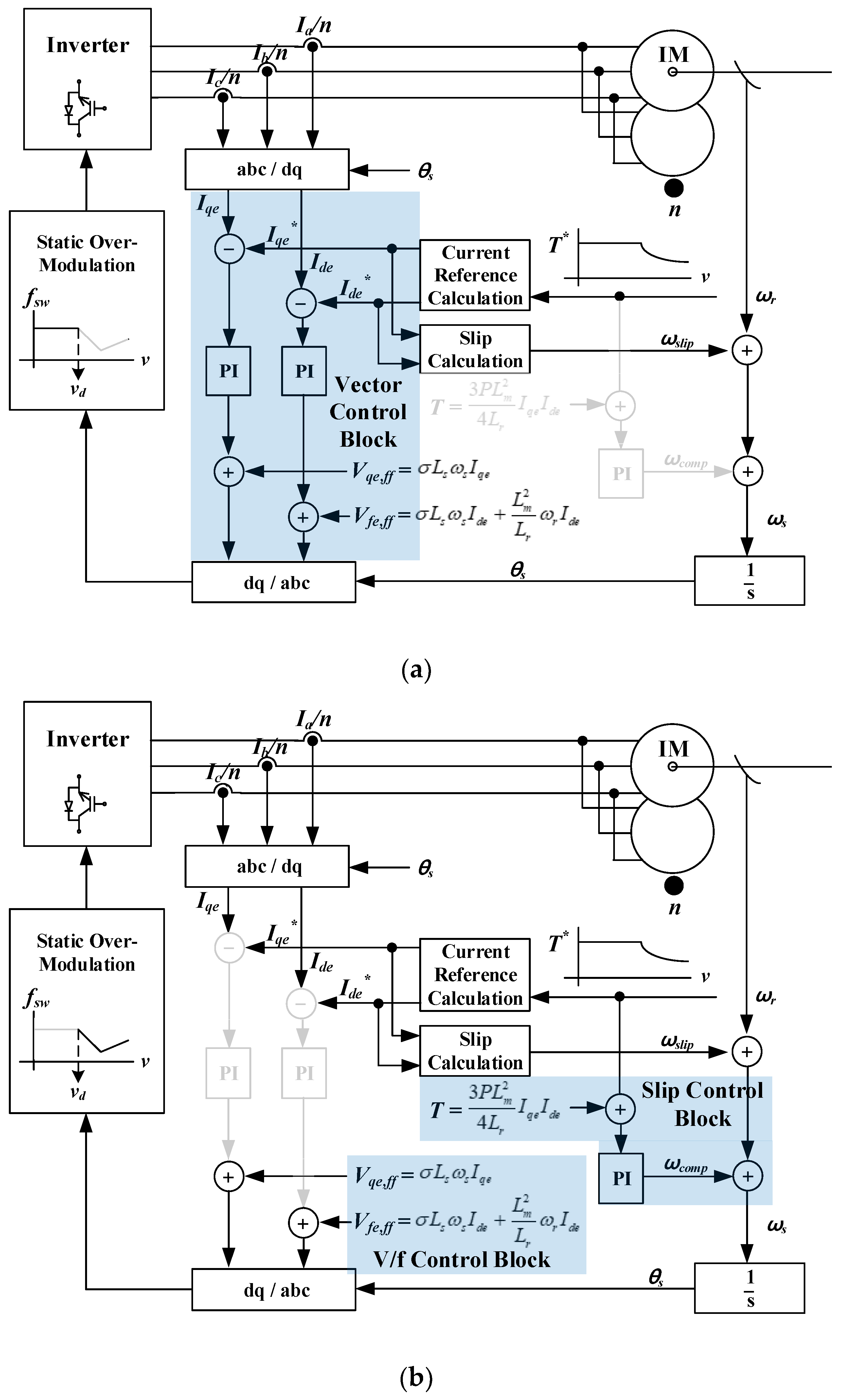
The power loss generated in the IGBT module is different depending on the control scheme and the mission profile of the railway system. Therefore, it is necessary to consider the control scheme of the inverter and the mission profile used in the railway train when the heat-pipe cooling system is designed.

2.1. Control Scheme

In the propulsion inverter of a railway system, the one-pulse switching method has been used in a wide operation range of induction motors [4,8]. The one-pulse switching method leads to a large torque ripple, which generates more vibration in a railway train than that using a carrier-based pulse-width modulation (PWM) method. Nevertheless, the one-pulse switching method shows the best performance in terms of power loss of the IGBT module. Furthermore, the vibration caused by the switching method can be ignored because the railway train has a large vibration itself through the mechanical structure between the rail and wheel of the train.
Figure 2 shows the control scheme used in the propulsion inverter of the railway system, where two control methods are combined. As shown in Figure 2a, the conventional vector control based on the carrier-based PWM is used in a low speed range of the induction motor [30,31]. The d-axis reference current (Ide*), meaning the flux and the q-axis reference current (Iqe*), indicate that the torque are calculated from the reference torque (T*). After the speed (v) of the induction motor increases until the defined speed (vd), the vector control is changed to the slip control with V/f control [32]. In the slip control, the slip is controlled from the torque error as shown in Figure 2b, and the reference voltages (Vde*, Vqe*) of the inverter increase as the speed (v) of induction motor increases. The carrier-based PWM method used in the vector control is applied continuously to the beginning of the slip control. Then, if the reference voltages (Vde*, Vqe*) are saturated due to their limited value (Vdc/2 or −Vdc/2), the one-pulse switching method is enabled. To guarantee the change in output voltages (Vxa, x = a, b, c) linearly, the static over-modulation method should be used [32].

2.2. Mission Profile

Railway trains run under a scheduled plan. The acceleration and deceleration values are the same at each station when the train departs and stops, respectively. Therefore, it is less complicated than an automotive car, which considers many scenarios [33].
Figure 3 shows the mission profile of the railway train between the stations and the train runs under the same mission profile repeatedly. The mission profile of the railway train can be divided into four sections. The first section is called acceleration, where the train departs from the station and speeds up to its maximum operation speed. The second is the coasting section, where the train runs by the inertia of the train without operating the propulsion system. Therefore, the speed of the train decreases slowly. The speed of the train is decelerated in the third section. In this section, the inverter operates as the generation (rectifier) mode since the power is generated from the wheel. In the last section, the train stops at the station. Consequently, the inverter operates in two sections, acceleration and deceleration.
In the acceleration section, the power (P) increases as the speed increases in the low speed range. This range is called the constant torque region. After the speed exceeds the base speed (vbase), which is the end of the constant torque region, P is maintained as the maximum value and the torque (T) decreases until v reaches the maximum speed. The magnitude of the current (|I|) has a constant value during the vector control. However, when the slip control is applied, it is changed because the magnitude of the current is not controlled. This works in a similar way in the deceleration part, but both T and P have negative values. As v increases, the switching method changes from the pulse-width modulation method to the over modulation method and one-pulse modulation method as shown in Figure 2. The switching frequency (fsw) is fixed in the pulse-width modulation range. The number of switching decreases in the over-modulation range and fsw is the same as the fundamental frequency of the motor current in the one-pulse modulation range. It is expected that the maximum power loss occurs at the end of the pulse-width modulation range.

3. Design Process of Heat-Pipe Cooling System

The design process of the heat-pipe cooling system used in a railway train is introduced in this section. Two criteria are taken into account: (1) The heat-pipe cooling system was exposed outside the train and the maximum external ambient temperature was assumed to be 318.15 K (45 °C), which is the maximum temperature of the external air (T5, tropical area except desert) in IEC 62498-1 [34]; (2) the junction temperature of the IGBT module cannot exceed the maximum allowed junction temperature of IGBT module; and (3) the 1 m/s wind, which is the average cooling effect generated by the running train to cool the heat-pipe cooling system. This is because the heat-pipe cooling system of the propulsion inverter is located at the bottom-left or -right side of the train and is exposed to the outside.

3.1. First Step: Power Loss Calculation Based on Control Scheme and Mission Profile

The first step is the power loss calculation of the IGBT module. The widely used 3300 V/1500 A IGBT module (Infineon, FZ1500R33HE3) in the propulsion inverter of a train was considered for the case study. Based on information obtained from the datasheet of FZ1500R33HE3, the power loss of the IGBT module was calculated when the inverter was operated under the given mission profile of a railway train with the control scheme introduced in Section 2. The total time of the mission profile was 128 s, acceleration time (ta) of the train was 48.5 s, coasting time (tc) of the train was 10 s, deceleration time (td) of train was 39.5 s, and the stopping time (ts) of train was 30 s. Table 1 shows the operation specifications for the propulsion system.

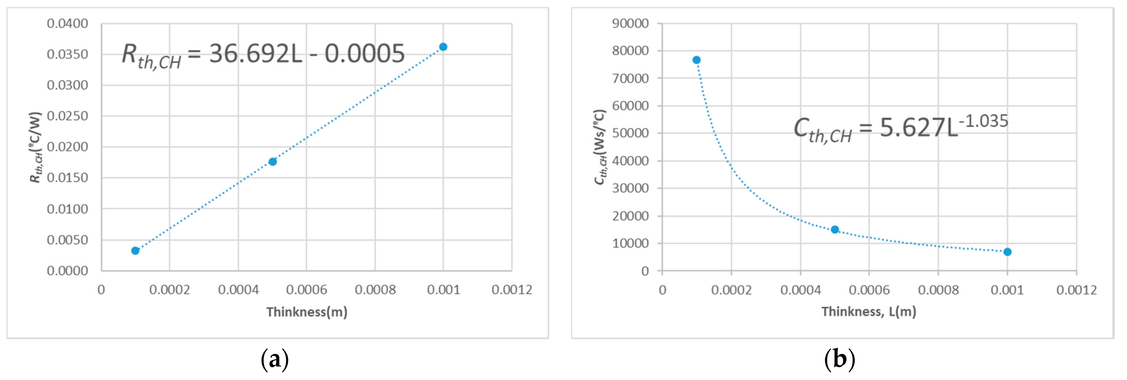
3.2. Second Step: Thermal Resistance Calculation of Heat-Pipe Cooling System Based on Junction Temperature of IGBT Module

In the second step, the thermal resistance of heat-pipe cooling system is calculated. The junction temperature of the IGBT module was estimated by the power loss of the IGBT module and the thermal equivalent circuit of the IGBT module with a heat-pipe cooling system in the propulsion inverter. The IGBT module was divided into two parts (IGBT and diode parts) and the thermal equivalent circuit was divided into the IGBT module (IGBT and diode parts), thermal grease, and heat-pipe, as shown in Figure 4 [29]. The IGBT and diode parts of the IGBT module are mainly influenced by each loss. However, the thermal grease and heap-pipe are related to both the IGBT and diode losses.
Figure 5 shows the four layer-Foster model, which represents the junction to case thermal impedances of the IGBT and diode in the IGBT module. This model consists of thermal resistances (Rth,IGBT,JCi, i = 1,2,3,4) and thermal capacitances (Cth,IGBT,JCi, I = 1,2,3,4) of the IGBT part and thermal resistances (Rth,Diode,JCi, i = 1,2,3,4) and thermal capacitances (Cth,Diode,JCi, i = 1,2,3,4) of the diode part. The parameters of the four layer-Foster model were from the datasheet of FZ1500R33HE3 and these parameters are shown in Table 2.
In the design process of a heat-pipe cooling system, the power loss (Ploss,IGBT) of the IGBT is only taken into account with the total thermal resistance (Rth,IGBT,JC) from the junction to case of the IGBT part to estimate the junction temperatures (Tj,IGBT) of the IGBT part in the module. This is because the Tj,Diode was lower than the Tj,IGBT from the thermal analysis of the IGBT module when the inverter was operated with the considered control scheme under the mission profile as shown in Table 3. To estimate the case temperature (TC) of the IGBT module from ambient temperature (TA), the total power loss (Ploss,module) of the IGBT module, which is the sum of Ploss,IGBT and the power loss (Ploss,Didoe) of the diode part, was applied to the thermal resistance (Rth,CH) of the thermal grease and thermal resistance (Rth,HA) of the heat-pipe cooling system. In this paper, the one layer-foster model was used for the thermal impedance of thermal grease. The thermal resistance (Rth,CH) and capacitance (Cth,CH) were acquired by the finite element method (FEM) analysis. In the FEM analysis, the dimension was fixed to attach two IGBT modules to the heat-pipe cooling system and the thermal parameters (Rth,CH and Cth,CH) were acquired according to the thickness (L) of the thermal grease, as shown in Figure 6.
The power loss and thermal resistance of IGBT module can determine the thermal resistance of heat-pipe cooling systems. The relationship between Tj,IGBT and temperature (THP) of the heat-pipe cooling system can be calculated from the thermal network in Figure 4 and is expressed as
T j , I G B T = R t h , I G B T , J C × P l o s s , I G B T + R t h , C H × P l o s s , m o d u l e + T H P .
The maximum allowed operation temperature (Tj,max) of the considered IGBT module is 423.15 K (150 °C) and the target junction temperature was set by considering the temperature design margin (Tmargin) as 30% of Tj,max. The required THP is expressed as
T H P T j , m a x T m a r g i n R t h , I G B T , J C × P l o s s , I G B T R t h , C H × P l o s s , m o d u l e .
The heat-pipe cooling system is designed from THP and Rth,HA is calculated as
R t h , H A = T H P T A P l o s s , m o d u l e = T j , m a x T m a r g i n R t h , I G B T , J C × P l o s s , I G B T R t h , C H × P l o s s , m o d u l e T A P l o s s , m o d u l e
where TA, which is the ambient temperature of 318.15 K (45 °C) in railway applications.

4. Heat-Pipe Cooling System Design

In this section, four heat-pipe cooling systems were designed according to different design processes. The relationship between the thermal impedance and power loss was introduced in Section 3, and based on this, the Rth,HA can be calculated by Equations (2) and (3). The two power losses (Ploss,IGBT and Ploss,module) used in Equations (2) and (3) are not instantaneous values. Using the instantaneous values of power losses for the design process of a heat-pipe cooling system is not desirable since all of the components (IGBT module, thermal grease, and heat-pipe cooling systems) have a thermal capacitance. The thermal capacitance determines how much the temperature increases during the fixed time. The effect of thermal capacitance on temperature variation will be analyzed in detail in the next section.
Two different average power losses during the period (tf) of fundamental current of inverter (or motor) and during the period (tm) of mission profile are taken into consideration in the heat-pipe cooling system design process. Figure 7 shows the power losses (Ploss,IGBT,tf and Ploss,module,tf) averaged for tf when the inverter is operated under the mission profile shown in Figure 3 with the control scheme shown in Figure 2. In the design process of the heat-pipe cooling system, the maximum values (Ploss,IGBT,tf,max and Ploss,module,tf,max) of Ploss,IGBT,tf and Ploss,module,tf are used to calculate Rth,HA. The power losses (Ploss,IGBT,tm and Ploss,module,tm) averaged for tm are easily calculated by integrating Ploss,IGBT,tf and Ploss,module,tf, for tm and are also considered to determine the required Rth,HA. Table 3 shows the different power losses used for heat-pipe cooling system design.
Two IGBT modules in a single leg were mounted on one heat-pipe cooling system. Therefore, Equation (3) for Rth,HA is modified as
R t h , H A = T H P T A P l o s s , m o d u l e = T j , m a x T m a r g i n R t h , I G B T , J C × P l o s s , I G B T R t h , C H × P l o s s , m o d u l e T A 2 × P l o s s , m o d u l e .
Four heat-pipe cooling systems were designed based on different combinations of power losses and the determined Rth,HAs are shown in Table 4. It can be seen that in Case 1, a minimum Rth,HA of 9.77 K/kW was required when the power losses averaged for tf are considered. In Case 4, the calculated Rth,HA was 50.03 K/kW, where the power losses averaged for tm were used. This was the maximum value among the four cases.

5. Comparison of Heat-Pipe Cooling Systems

Four heat-pipe cooling systems were compared in terms of design feasibility, size, and weight. Furthermore, the lifetime of the IGBT module in the propulsion inverter with four different heat-pipe cooling systems were estimated and compared.

5.1. Design Feasibility

Four heat-pipe cooling systems were designed by setting the target junction temperature as 342.15 K (105 °C), which is Tj,maxTmargin. Figure 8 shows the junction temperature of the IGBT module with four heat-pipe cooling systems when the train is operated as shown in Figure 7. In Figure 7 and Figure 8, as the train speed increases, the control scheme changes. At the low speed range, the carrier based PWM is applied; therefore, the three-phase currents (Ix, x = a, b, c) have the ripple component of carrier frequency. As the speed increases, the over-modulation is identified through the gate signal of Sap and extended to the one-pulse switching method. The junction temperature of the start point in acceleration is lower than that of the end point in deceleration. This is because the magnitude (Imag) of the reference current shown in Figure 9 increased slowly at the start point in acceleration, but the peak value of Imag was maintained at the end point in deceleration, as shown in Figure 9. The same performances in motor currents, motor torque, and motor speed of the propulsion inverter were identified in four cases.
In Case 1, it can be seen that the maximum junction temperature of the IGBT during the mission profile was lower by about 293.15 K (20 °C) than the target junction temperature. This means that the heat-pipe cooling system is over designed, if Ploss,module,tf,max is used only. The maximum junction temperature of the IGBT with the heat-pipe cooling system in Case 2 was almost the same with the target junction temperature. In Cases 3 and 4, the maximum junction temperatures of the IGBT exceeded the target junction temperature more than 288.15 K (15 °C) and 298.15 K (25 °C), respectively, which may cause safety issues. From the above results, it can be concluded that the heat-pipe cooling system designed as Case 2 is the most appropriate for this railway train system.
Figure 10 shows the effect of thermal capacitances on junction temperature variation. The temperature differences between the junction and case, case and heat-pipe cooling system, and heat-pipe cooling system and ambient had different thermal capacitance values. The IGBT module had smallest thermal capacitance (Cth,IGBT,JC) of about 3.8 kWs/K; therefore, Tj,IGBT was changed immediately by the variation of the power loss. On the contrary, the heat-pipe cooling system had the largest thermal capacitance of about 217 kWs/K. Therefore, it prevented THP from changing quickly. As the thermal capacitance is larger, the slope of temperature difference is small.

5.2. Size and Weight of Heat-Pipe Cooling Systems

Four cases had differences in thermal resistance respectively. This means that the size and weight of the four cases were different. To compare them in terms of size and weight, the dimension of the surface where two IGBT modules were mounted was defined as 460 mm × 260 mm. The height of the heat-pipe cooling system only changed depending on the value of the thermal resistance. Figure 11 shows the 3D model of the heat-pipe cooling system designed for Case 2. The specifications of the 3D model for the heat-pipe cooling system are shown in Table 5. The height of the heat-pipe cooling system for Case 2 was 490 mm and satisfies the required thermal resistance of 33.12 K/kW.
Figure 12 shows the finite element method (FEM) analysis result at the power loss of 525 W per IGBT module. The ambient temperature was 318.15 K (45 °C) and a wind of 1 m/s was applied. The maximum temperature was 80.49 °C and it was identified that the heat-pipe cooling system in Figure 12 had (353.64 K (80.49 °C) − 318.15 K (45 °C)) × (525 W × 2) of the thermal resistance, which is the required value for Case 2.
The size and weight depending on the heat-pipe cooling system are summarized in Table 6. They were acquired from the finite element method (FEM) analysis result and satisfied the required thermal resistance. As the thermal resistance is small, the size and weight increased.

5.3. Lifetime Estimation of the IGBT Module

In this section, the lifetime of the IGBT module with four different heat-pipe cooling systems are estimated and compared.
It is worth noticing that the temperature stress was considered when the lifetime estimation of IGBT module was carried out because it is the main cause of the wear-out failure of standard IGBT modules. Furthermore, the lifetime estimation was focused on the IGBT part since the power losses of the IGBTs were dominant, and thus it had a higher junction temperature stress than the diode part as mentioned in Section 3.2. Consequently, a shorter lifetime than that of the diode is expected. Typically, the temperature stress factors, which are the junction temperature variation (ΔT) of IGBT module, minimum junction temperature (Tj,min), and the duration (ton) of ΔT, are considered when the lifetime is estimated based on the lifetime model. These factors were extracted from the junction temperature profiles as illustrated in Figure 8 by the rainflow counting method [24]. Then, the stress factors such as the junction temperature variation (ΔT) of IGBT module, minimum junction temperature (Tj,min), and the duration (ton) of ΔT were extracted from the junction temperature profile by the rainflow counting method. [24]. Then, the lifetime of the IGBT module was estimated from the accumulated damage based on Miner’s rule by putting the extracted temperature stress factors into a lifetime model.
Accumulated damage (AD) of the IGBT module was calculated based on Miner’s rule, which is one of the most widely used cumulative damage models and is defined as
D A = i = 1 k n i N i
where ni is the number of cycles accumulated at a certain temperature stress Si, which consists of △Tj, Tjmin, and ton, and Nfi is the number of cycles to failure at the temperature stress Si and is calculated from the lifetime model of the IGBT module.
Since there is no lifetime model for the target IGBT module, the existing lifetime model presented in [28] is used in this study as
N f = A ( Δ T j ) β 1 exp ( β 2 T j , min + 273.15 ) ( t on ) β 3 ( I B ) β 4 ( V c ) β 5 ( D ) β 6
where Nf is the number of cycles to failure, and others are defined as shown in Table 7.
Finally, the lifetime of the IGBT module can be obtained as
L i f e t i m e ( d a y ) = P e r i o d o f m i s s i o n p r o f i l e ( s ) O p e r a t i n g t i m e ( s ) × A c c u m u l a t e d d a m a g e
Four average ambient temperatures depending on the season were taken into account as shown in Table 8, when the junction temperature profiles of the IGBT module with four heat-pipe cooling systems were obtained.
Figure 13 shows three stress factors (ΔT, Tj,min, ton) extracted by the rainflow counting method in the summer season of Case 1 and Case 4 of the heat-pipe cooling systems. Since the thermal resistance of Case 4 was bigger than that of Case 1, the Tj,min of Case 4 was higher than that of Case 1. However, the ΔT and ton in Case 1 and Case 4 were similar.
The three stress factors of Case 2, depending on the season, are shown in Figure 14. Since they applied different ambient temperatures to obtain the junction temperature of the IGBT module, each figure has a different Tj,min.
The extracted data of the stress factors resulted in AD during one mission profile. Table 9 shows the AD for four heat-pipe cooling systems depending on the season. In all cases, the winter season had the lowest AD of the IGBT module and the summer season, which had the highest ambient temperature, showed the highest AD of the IGBT module in all heat-pipe cooling systems. The autumn and spring seasons had similar AD because the ambient temperatures were similar. The rise of the ambient temperature resulted in increasing Tj(min) and it was identified that Nf of Equation (6) is reduced when Tj(min) increases. Consequentially, the high TA increases the AD of the IGBT module. In addition, Case 1, which had the lowest thermal resistance of heat-pipe cooling system, had the lowest AD damage. As the thermal resistance of the heat-pipe cooling system increases, the AD of the IGBT module increases. In the summer season, the AD of Case 4 was two times bigger when compared to Case 1.
The lifetime of IGBT module can be calculated by using AD, as summarized in Table 9 and Equation (7). This paper assumed that the operating time of the train was 8 h per day. This means that the mission profile repeats 225 times per day. The lifetimes of the IGBT modules, depending on heat-pipe cooling system, were calculated as shown in Table 10.

6. Conclusions

This paper reviewed the existing design processes for heat-pipe cooling systems. Based on the processes, two power losses averaged during the period (tf) of the fundamental current of the inverter and the period (tm) of the mission profile are considered to calculate the thermal resistance of a heat-pipe cooling system. As a result, the four heat-pipe cooling system was designed and compared in terms of the design feasibility, and the size and weight of the heat-pipe. In addition, the lifetime of the IGBT module in the propulsion inverter was estimated.
Four thermal resistances for the heat-pipe cooling system design are summarized in Table 11. The design accuracy was defined as [1 − (|Real junction temperature − Target junction temperature|)/Target junction temperature × 100%]. Case 2, which uses Ploss,IGBT,tf,max for Rth,IGBT,jc, Ploss,module,tf,max for Rth,CH, and Ploss,module for Rth,HA, had good accuracy in the heat-pipe cooling system design for the train propulsion system. In addition, the lifetime of Case 2 was over 20 (years), which is the required value in the train application.

Author Contributions

U.-M.C. provided guidance and supervision. J.-S.L. implemented the main research, performed the simulation, wrote the paper, and revised the manuscript as well. All authors have equally contributed to the simulation analysis and result discussions.

Funding

This work was supported by the Railroad Technology Research Program funded by Ministry of Land, Infrastructure and Transport of Korean Government under Grant 19RTRP-B146008-02.

Conflicts of Interest

The authors declare no conflict of interest.

Nomenclature

IGBTInsulated gate bipolar mode transistor
MTBFMean time between failures
PWMPulse-width modulation
FEMFinite element method
Ide*d-axis reference current of motor
Iqe*q-axis reference current of motor
T*Reference torque of motor
vSpeed of induction motor
vdDefined speed for changing control scheme
vbaseBase speed of induction motor
Vde*, Vqe*d-/q-axis reference voltages of inverter
Vxa, x = a, b, cOutput voltages of inverter
PPower of motor
TTorque of motor
fswSwitching frequency of inverter
taAcceleration time of train
tcCoasting time of train
tdDeceleration time of train
tsStopping time of train
Rth,IGBT,JCi, Cth,IGBT,JCi,i = 1,2,3,4Thermal resistances and capacitances of IGBT part
Rth,Diode,JCi, Cth,Diode,JCi,i = 1,2,3,4Thermal resistances and capacitances of diode part
Rth,IGBT,JCTotal thermal resistance of IGBT part
Cth,IGBT,JCTotal thermal capacitance of IGBT part
Rth,CHThermal resistance of thermal grease
Cth,CHThermal capacitance of thermal grease
Rth,HAThermal resistance of heat-pipe cooling system
Tj,maxMaximum allowed operation temperature of IGBT module
TmarginTemperature design margin
Tj,IGBTJunction temperatures of IGBT part
TCCase temperature of IGBT module
THPTemperature of heat-pipe cooling system
TAAmbient temperature
tfPeriod of fundamental current of inverter
tmPeriod of mission profile
Ploss,IGBTPower loss of IGBT part
Ploss,DidoePower loss of Diode part
Ploss,moduleTotal power loss of IGBT module
Ploss,IGBT,tf, Ploss,module,tfPower losses of IGBT and Diode averaged for tf
Ploss,IGBT,tf,max, Ploss,module,tf,maxMaximum values of Ploss,IGBT,tf and Ploss,module,tf
Ploss,IGBT,tm, Ploss,module,tmPower losses of IGBT and Diode averaged for tm

References

  1. Skudelny, H.; Weinhardt, M. An investigation of the dynamic response of two induction motors in a locomotive truck fed by a common inverter. IEEE Trans. Ind. Appl. 1984, 1, 173–179. [Google Scholar]
  2. Youssef, M.Z.; Woronowicz, K.; Aditya, K.; Azeez, N.A.; Williamson, S.S. Design and development of an efficient multilevel DC/AC traction inverter for railway transportation electrification. IEEE Trans. Power Electron. 2016, 4, 3036–3042. [Google Scholar] [CrossRef]
  3. Calleja, C.; L’opez-de-Heredia, A.; Gaztanaga, H.; Aldasoro, L.; Txomin, N. Validation of a modified direct-self-control strategy for PMSM in railway—Traction applications. IEEE Trans. Ind. Electron. 2016, 8, 5143–5155. [Google Scholar] [CrossRef]
  4. Liu, J.; Zhang, W.; Lian, C.; Gao, S. Six-step mode control of IPMSM for railway vehicle traction eliminating the DC offset in input current. IEEE Trans. Power Electron. 2019, 9, 8981–8993. [Google Scholar] [CrossRef]
  5. Broche, C.; Lobry, J.; Colignon, P.; Labart, A. Harmonic reduction in DC link current of a PWM induction motor drive by active filtering. IEEE Trans. Power Electron. 1992, 10, 633–643. [Google Scholar] [CrossRef]
  6. Ouyang, H.; Zhang, K.; Zhang, P.; Kang, Y.; Xiong, J. Repetitive compensation of fluctuating dc link voltage for railway traction drives. IEEE Trans. Power Electron. 2011, 8, 2160–2171. [Google Scholar] [CrossRef]
  7. Ronanki, D.; Singh, S.A.; Williamson, S.S. Comprehensive topological overview of rolling stock architectures and recent trends in electric railway traction systems. IEEE Trans. Transport. Electrific. 2017, 9, 724–738. [Google Scholar] [CrossRef]
  8. Diao, L.; Tang, J.; Loh, H.C.; Yin, Y.; Wang, L.; Liu, Z. An efficient DSP–FPGA-based implementation of hybrid PWM for electric rail traction induction motor control. IEEE Trans. Power Electron. 2018, 4, 3276–3288. [Google Scholar] [CrossRef]
  9. Perpiñà, X.; Jordà, X.; Vellvehi, M.; Rebollo, J.; Mermet-Guyennet, M. Long-Term reliability of railway power inverters cooled by heat-pipe-based systems. IEEE Trans. Ind. Electron. 2011, 7, 2662–2672. [Google Scholar]
  10. Andresen, M.; Ma, K.; Buticchi, G.; Falck, J.; Blaabjerg, F.; Liserre, M. Junction temperature control for more reliable power electronics. IEEE Trans. Power Electron. 2018, 1, 765–776. [Google Scholar] [CrossRef] [Green Version]
  11. Shabgard, H.; Bergman, T.L.; Sharifi, N.; Faghri, A. High temperature latent heat thermal energy storage using heat pipes. Int. J. Heat Mass Transf. 2010, 7, 2979–2988. [Google Scholar] [CrossRef]
  12. Esarte, J.; Blanco, J.M.; Bernardini, A.; San José, J.T. Optimizing the design of a two-phase cooling system loop heat pipe: Wick manufacturing with the 3D selective laser melting printing technique and prototype testing. Appl. Therm. Eng. 2017, 1, 407–419. [Google Scholar] [CrossRef]
  13. Deng, S.; Li, K.; Xie, Y.; Wu, C.; Wang, P.; Yu, M.; Li, B.; Zheng, J. Heat pipe thermal management based on high-rate discharge and pulse cycle tests for lithium-ion batteries. Energies 2019, 12, 3413. [Google Scholar] [CrossRef] [Green Version]
  14. Chi, R.G.; Rhi, S.H. Oscillating heat pipe cooling system of electric vehicle’s li-ion batteries with direct contact bottom cooling mode. Energies 2019, 12, 1698. [Google Scholar] [CrossRef] [Green Version]
  15. Hamidi, A.; Coquery, G.; Lallemand, R.; Vales, P.; Dorkel, J.M. Temperature measurements and thermal modeling of high power IGBT multichip modules for reliability investigations in traction applications. Microelectron. Reliab. 1998, 38, 1353–1359. [Google Scholar] [CrossRef]
  16. Watanabe, T.; Fukuda, N. Reliability of Power Converters—Lifetime Cycle Approach. In Proceedings of the 14th International Power Electronics and Motion Control Conference (EPE-PEMC), Ohrid, Macedonia, 6–8 September 2010; pp. S8–10–11. [Google Scholar]
  17. Perpiñà, X.; Serviere, J.F.; Urresti-Ibañez, J.; Cortés, I.; Jordà, X.; Hidalgo, S.; Rebollo, J.; Mermet-Guyennet, M. Analysis of clamped inductive turnoff failure in railway traction IGBT power modules under overload conditions. IEEE Trans. Ind. Electron. 2011, 7, 2706–2714. [Google Scholar]
  18. Ouni, F.; Ammar, F.B. Reliability Estimation of Sahel Tunisian Railway Drive System. In Proceedings of the 16th IEEE Mediterranean Electrotechnical Conference, Yasmine Hammamet, Tunisia, 25–28 March 2012; pp. 614–617. [Google Scholar]
  19. Hayashiya, H.; Masuda, M.; Noda, Y.; Suzuki, K.; Suzuki, T. Reliability Analysis of DC Traction Power Supply System for Electric Railway. In Proceedings of the 19th European Conference on Power Electronics and Applications (EPE’17 ECCE Europe), Warsaw, Poland, 11–14 September 2017; pp. 1–6. [Google Scholar]
  20. Choi, U.M.; Blaabjerg, F.; Jørgensen, S. Power cycling test methods for reliability assessment of power device modules in respect to temperature stress. IEEE Trans. Power Electron. 2018, 3, 2531–2551. [Google Scholar] [CrossRef] [Green Version]
  21. Ma, K.; Liserre, M.; Blaabjerg, F.; Kerekes, T. Thermal loading and lifetime estimation for power device considering mission profiles in wind power converter. IEEE Trans. Power Electron. 2015, 2, 590–602. [Google Scholar] [CrossRef]
  22. Shipurkar, U.; Lyrakis, E.; Ma, K.; Polinder, H.; Ferreira, J.A. Lifetime comparison of power semiconductors in three-level converters for 10-MW wind turbine systems. IEEE Trans. Power Electron. 2018, 9, 1366–1377. [Google Scholar] [CrossRef]
  23. Alhmoud, L. Reliability improvement for a high-power IGBT in wind energy applications. IEEE Trans. Ind. Electron. 2018, 9, 7129–7137. [Google Scholar] [CrossRef]
  24. GopiReddy, L.R.; Tolbert, L.M.; Ozpineci, B.; Pinto, J.O.P. Rainflow algorithm-based lifetime estimation of power semiconductors in utility applications. IEEE Trans. Ind. Appl. 2015, 7, 3368–3375. [Google Scholar] [CrossRef]
  25. Ma, K.; Choi, U.M.; Blaabjerg, F. Prediction and validation of wear-out reliability metrics for power semiconductor devices with mission profiles in motor drive application. IEEE Trans. Power Electron. 2018, 11, 9843–9853. [Google Scholar] [CrossRef] [Green Version]
  26. Choi, U.M.; Vernica, I.; Blaabjerg, F. Effect of asymmetric layout of IGBT modules on reliability of motor drive inverters. IEEE Trans. Power Electron. 2019, 2, 1765–1772. [Google Scholar] [CrossRef] [Green Version]
  27. Choi, U.M.; Ma, K.; Blaabjerg, F. Validation of lifetime prediction of IGBT modules based on linear damage accumulation by means of superimposed power cycling tests. IEEE Trans. Ind. Electron. 2018, 4, 3520–3529. [Google Scholar] [CrossRef]
  28. Wintrich, A.; Nicolai, U.; Tursky, W.; Reimann, T. Application Manual Power Semiconductors; SEMIKRON International GmbH: Nuremberg, Germany, 2015. [Google Scholar]
  29. Ma, K.; Blaabjerg, F.; Liserre, M. Thermal loading and reliability of 10-MW multilevel wind power converter at different wind roughness classes. IEEE Trans. Ind. Appl. 2013, 3, 909–921. [Google Scholar] [CrossRef]
  30. Quraan, M.; Siam, J. Modeling and Simulation of Railway Electric Traction with Vector Control Drive. In Proceedings of the IEEE International Conference on Intelligent Rail Transportation (ICIRT), Birmingham, UK, 23–25 August 2016; pp. 1–6. [Google Scholar]
  31. Peroutka, Z.; Zeman, L. New Field Weakening Strategy for AC Machine Drives for Light Traction Vehicles. In Proceedings of the European Conference on Power Electronics and Applications, Aalborg, Denmark, 2–5 September 2007; pp. 1–10. [Google Scholar]
  32. Yanol, M.; Iwahori, M. Transition from Slip-Frequency Control to Vector Control for Induction Motor Drives of Traction Applications in Japan. In Proceedings of the Fifth International Conference on Power Electronics and Drive Systems (PEDS), Singapore, 17–20 November 2003; pp. 1246–1251. [Google Scholar]
  33. Martinez, C.M.; Heucke, M.; Wang, F.Y.; Gao, B.; Cao, D. Driving style recognition for intelligent vehicle control and advanced driver assistance: A survey. IEEE Trans. Intell. Syst. 2018, 3, 666–676. [Google Scholar] [CrossRef] [Green Version]
  34. IEC 62498-1. Railway Applications—Environmental Conditions for Equipment—Part 1: Equipment on Board Rolling Stock, 1st ed.; IEC 62498-1: Geneva, Switzerland, 2010. [Google Scholar]
Figure 1. The configuration of the propulsion system: single inverter and multiple induction motors.
Energies 12 04676 g001
Figure 2. Control scheme applied in the propulsion inverter of railway system: (a) Vector control when v is smaller than vd; (b) Slip control with V/f control when v is larger than vd.
Energies 12 04676 g002
Figure 3. Mission profile of an urban railway train.
Energies 12 04676 g003
Figure 4. Thermal equivalent circuit.
Energies 12 04676 g004
Figure 5. The 4 layer-foster model of the IGBT module.
Energies 12 04676 g005
Figure 6. Thermal impedance of thermal grease (Parker Chomerics, T660), depending on the thickness (L). (a) Rth,ch, (b) Cth,ch.
Energies 12 04676 g006
Figure 7. The average power loss for tf.
Energies 12 04676 g007
Figure 8. Junction temperature of the IGBT depending on the heat-pipe cooling system.
Energies 12 04676 g008
Figure 9. The magnitude variation of the reference current (Imag) during the mission profile.
Energies 12 04676 g009
Figure 10. The effect of thermal capacitances.
Energies 12 04676 g010
Figure 11. 3D module of the heat-pipe cooling system for Case 2 (thermal resistance was 33.12 K/kW).
Energies 12 04676 g011
Figure 12. Finite element method (FEM) analysis result with the heat-pipe cooling system for Case 2 (thermal resistance was 33.12 K/kW and 525 W per IGBT module).
Energies 12 04676 g012
Figure 13. Three stress factors in the summer season. (a) Case 1. (b) Case 4.
Energies 12 04676 g013
Figure 14. Three stress factors of Case 2. (a) Spring. (b) Summer. (c) Autumn. (d) Winter.
Energies 12 04676 g014
Table 1. The operation specifications for the propulsion system.
SpecificationValue
IGBT moduleVoltage/Current3300 V/1500 A
Control SchemeDC-link voltage1500 V
Maximum current (only at vector control)860 Apeak
Switching frequency800 Hz
Defined speed (vd) for changing control1056 rpm (23 km/h of train)
Base speed (vbase) 1800 rpm (39 km/h of train)
MotorThe number of motors connected to inverter 4
Rated torque per induction motor900 Nm
Pole4
Magnetizing inductance0.0225 H
Table 2. Thermal equivalent parameters of the IGBT module (FZ1500R33HE3).
Junction to caseiIGBT PartDiode Part
Rth,IGBT,JCi (K/W)Cte,IGBT,JCi (Ws/K)Rth,Diode,JCi (K/W)Cth,Diode,JCi (Ws/K)
10.00130.0024140.8285
20.00386910.8555180.0062665.745292
30.00146175.3424660.00278790.419806
40.0010024974.0518960.0015093702.4519549
Table 3. The different power losses used for heat-pipe cooling system design.
IGBT PartDiode PartIGBT Module
Ploss,IGBT,tf,maxPloss,IGBT,tmPloss,Didoe,tf,maxPloss,Diode,tmPloss,module,tf,maxPloss,module,tm
Power loss1656.49 W379.39 W630.89 W155.9 W1813.77 W535.29 W
Table 4. Four heat-pipe cooling systems with different thermal resistance (Rth,HA).
CaseTj,maxTmarginTAThickness of Thermal GreaseMultiplied Power Loss for Rth,IGBT,jcMultiplied Power Loss for Rth,CHMultiplied Power Loss for Rth,HARth,HA
1423.15 K318.15 K318.15 K0.0002 mPloss,IGBT,tf,maxPloss,module,tf,maxPloss,module,tf,max9.77 K/kW
2Ploss,IGBT,tf,maxPloss,module,tf,maxPloss,module,tm33.12 K/kW
3Ploss,IGBT,tf,maxPloss,module,tmPloss,module,tm41.28 K/kW
4Ploss,IGBT,tmPloss,module,tmPloss,module,tm50.03 K/kW
Table 5. Specifications of the heat-pipe cooling system.
SpecificationMaterialDimension
Baseplate of heat-pipe cooling systemAluminum (A6063)22.5 mm (Thickness)
Fin of heat-pipe cooling systemAluminum (A6063)0.8 mm (Thickness)
Heat-pipe of heat-pipe cooling system Copper16 mm (Diameter)
Table 6. Size and weight of the four heat-pipe cooling system.
CaseRth,HASize (W × D × H)Weight
19.77 K/kW460 mm × 260 mm × 494 mm48.3 kg
233.12 K/kW460 mm × 260 mm × 490 mm43.6 kg
341.28 K/kW460 mm × 260 mm x 449 mm41.6 kg
450.03 K/kW460 mm × 260 mm × 390 mm38.7 kg
Table 7. Definition of parameters used in the lifetime module (6) of the IGBT module.
ParameterSymbolCoefficient Value
Technology FactorA-
Temperature difference (K)△Tβ1
Min. chip temperature (K)Tj,minβ2
Pulse duration (s)tonβ3
Current per bond foot (A)IBβ4
Voltage class/100 (V)VCβ5
Bond wire diameter (μm)Dβ6
Table 8. The averaged ambient temperatures depending on the season.
SeasonTemperature
Spring286.6 K (13.45 °C)
Summer300.17 K (27.02 °C)
Autumn287.74 K (14.58 °C)
Winter271.42 K (−1.73 °C)
Table 9. Accumulated damage (AD) of the IGBT module.
SeasonAccumulated Damage (AD)
Case 1Case 2Case 3Case 4
Spring3.633 × 10−75.205 × 10−76.044 × 10−76.912 × 10⁻⁷
Summer4.348 × 10−76.534 × 10−78.108 × 10−78.712 × 10⁻⁷
Autumn3.794 × 10−75.374 × 10−76.242 × 10−77.230 × 10⁻⁷
Winter3.742 × 10−74.324 × 10−74.809 × 10−75.389 × 10⁻⁷
Table 10. Lifetime of the IGBT module depending on the heat-pipe cooling system.
SeasonLifetime (year)
Case 1Case 2Case 3Case 4
Spring32.623.7520.4517.9
Summer28.4418.9215.2514.2
Autumn34.032319.8117.1
Winter33.0428.625.7222.9
Averaged3223.620.318
Table 11. Comparison results of the four heat-pipe cooling system.
CaseDesign AccuracyLifetimeSize/Weigh
180%32 year460 mm × 260 mm × 494 mm/48.3 kg
296%23.6 year460 mm × 260 mm × 490 mm/43.6 kg
386%20.3 year460 mm × 260 mm × 449 mm/41.6 kg
477%18 year460 mm × 260 mm × 390 mm/38.7 kg

