Article

Effect of Viscous Dissipation in Heat Transfer of MHD Flow of Micropolar Fluid Partial Slip Conditions: Dual Solutions and Stability Analysis

1
School of Quantitative Sciences, Universiti Utara Malaysia, Sintok 06010, Kedah
2
KCAET Khairpur Mir’s & FAE, Sindh Agriculture University, Tandojam 70060, Pakistan
3
Faculty of Mathematics and Statistics, Ton Duc Thang University, Ho Chi Minh City 72915, Vietnam
4
Department of Mathematics and Computer Science, Beirut Arab University, 115020 Beirut, Lebanon
5
Department of Software, Sejong University, Seoul 05006, Korea
6
Department of Mathematics, College of Arts and Sciences, Prince Sattam bin Abdulaziz University, Wadi Al-Dawaser 11991, Saudi Arabia
*
Author to whom correspondence should be addressed.
Energies 2019, 12(24), 4617; https://doi.org/10.3390/en12244617
Submission received: 28 October 2019 / Revised: 20 November 2019 / Accepted: 28 November 2019 / Published: 5 December 2019
(This article belongs to the Special Issue Fluid Flow and Heat Transfer Ⅱ)

Abstract

:
In this study, first-order slip effect with viscous dissipation and thermal radiation in micropolar fluid on a linear shrinking sheet is considered. Mathematical formulations of the governing equations of the problem have been derived by employing the fundamental laws of conservations which then converted into highly non-linear coupled partial differential equations (PDEs) of boundary layers. Linear transformations are employed to change PDEs into non-dimensional ordinary differential equations (ODEs). The solutions of the resultant ODEs have been obtained by using of numerical method which is presented in the form of shootlib package in MAPLE 2018. The results reveal that there is more than one solution depending upon the values of suction and material parameters. The ranges of dual solutions are S     S c i , i   =   0 ,   1 ,   2 and no solution is S   <   S c i where S c i is the critical values of S . Critical values have been obtained in the presence of dual solutions and the stability analysis is carried out to identify more stable solutions. Variations of numerous parameters have been also examined by giving tables and graphs. The numerical values have been obtained for the skin friction and local Nusselt number and presented graphically. Further, it is observed that the temperature and thickness of the thermal boundary layer increase when thermal radiation parameter is increased in both solutions. In addition, it is also noticed that the fluid velocity increases in the case of strong magnetic field effect in the second solution.

1. Introduction

The study of the magnetohydrodynamic flow of non-Newtonian fluids has fascinated many scientists, researchers and mathematicians because there are numerous technical applications of non-Newtonian material such as greases, processed food, paints, ketchup, dyes, etc., [1]. The relation of shear stress and strain is non-linear the fluid is said to be a non-Newtonian fluid. Moreover, the dealing with the non-Newtonian fluid is more complicated as compared to Newtonian as the equation of Navier Stokes is related to many constraints, other physical parameters, and numbers [2]. It is not possible that one fluid model keeps all characteristics of the non-Newtonian fluid. Therefore, researchers introduced many non-Newtonian models such as model of Casson [3,4], Micropolar [5,6], Maxwell [7,8]; Jeffrey [9,10]; Burgers [11,12], etc. The micropolar model was introduced by Eringen in 1966 [13] in which he added the microrotation effect in the equation of Navier Stokes as the equation of Navier Stokes fails to interpret the behavior of such fluids. The micropolar fluid was examined by Bhattacharjee et al. [14] in which they also considered the porous effects and found only a single solution. Koriko et al. [15] investigated the micropolar fluid in the presence of thermal effects. Lakshmi et al. [16] studied the micropolar fluid and its heat characteristics by consideration of the second slip effect. Further, the following advanced studies have been carried out for micropolar fluids [17,18,19,20,21,22]. It is worth to note that the focus of all the above-mentioned studies is only in a single solution. Few related studies of micropolar fluid can be seen in these articles in which authors found multiple solutions successfully [23,24,25,26,27]. It has been concluded from the vast survey of published literature that the multiple solutions of micropolar fluid with the effect of viscous dissipation, thermal radiation and slip effect has not been studied so far.
Nowadays, nonlinear boundary values problems (BVPs) of fluid flows and their multiple solutions are important due to their wide applications in engineering and scientific research. In light of the nonlinear problems and their solutions, there may exist multiple solutions in numerous nonlinear fluid flow problems whose all possible solutions are hard to find [28]. Since all possible solutions satisfy the solution conditions of the considered fluid flow problems, it is essential not neglect any solution. Unfortunately, most of the current numerical techniques fail to recognize the multiple solutions because they are near to each other and may oscillate between two adjacent solutions [28]. These solutions exist in boundary layer fluid flow problems due to non-linearity in equations [29,30] as encountered in material science, electrochemistry, viscoelasticity, electro-magnetics, and acoustics. Soid et al. [31] considered steady MHD flow over a radially stretching or shrinking disk and noticed that dual solutions only exist on shrinking surface with small values of suction and the magnetic parameters. Khan et al. [32] investigated Carreau nanofluids and found the dual solutions by using the BVP4C method in MATLAB 2017 version. Raju et al. [33] discovered that dual solution exists only in a certain range of Power-law index values and found that reduction in the coefficient of skin friction and heat transfer rate due to increments in a field of a magnetic parameter. Lok et al. [34] examined the stagnation point flow of micropolar fluid and found dual solutions. Dual solutions of micropolar fluid in the presence of chemical reaction were investigated by Sandeep et al. [35]. Yacob et al. [36] found two solutions for the shrinking case when they dealt with micropolar fluid with the effect of stagnation. Turkyilmazoglu [37] extended the work of Bhattacharyya et al. [38] and found dual solutions of micropolar fluid in exact form. From an extensive review of published literature, it is noticed that micropolar fluid with the effect of partial slip conditions and viscous dissipation has not been investigated for the case of multiple solutions. Therefore, the main aim of this study is to find all possible solutions of MHD flow of the micropolar fluid with slip effect over a linear shrinking surface.
In the present decade, multiple solutions are considered in the fluid flow problem due to their wide range of applications in different areas of industries, engineering and so on. In order to determine which solution is physically realizable and stable, the stability analysis is employed by several researchers in their works. Based on the published works, Wilks and Bramley [39] were the first who found dual solutions in mixed convection flow and performed stability analysis of the solutions. After that, Merkin [40] also found the dual solutions in the fluid flow problem of mixed convection in a porous medium and carried out stability analysis to indicate that the first solution is more stable. The general definition of the theory of stability is regarded with measuring the behavior of perturbations of infinitesimal around the base state of finite-amplitude. If the perturbed flow returns to the base state, the flow is considered stable. On the other hand, if the small-amplitude perturbations diverge from the base state, the flow is considered unstable. Recently, Ali et al., [41] performed the stability analysis for MHD mixed convection flow of viscous fluid on the vertical surface and found that the first solution is a stable one. Lund et al. [42] examined the Williamson fluid, found dual solutions, and performed stability analysis. Khan et al. [43] investigated the non-Newtonian fluid and did stability analysis in order to indicate stable solutions. With existence of generation and absorption of heat, Jusoh et al. [44] found multiple solutions and examined the stability of solutions. Triple solutions have been found for the micropolar nanofluid over shrinking surfaces by Lund et al. [45]. The results of stability analysis exposed that only stable solution is the first one and the remaining two solutions are unstable. However, many researchers who found multiple solutions in fluid flow problems did not conduct this analysis [35,46,47,48]. It is worth to highlight that stability analysis should be considered in fluid flow problems when multiple solutions occur. Thus, this analysis is considered in this study to determine a more stable solution.

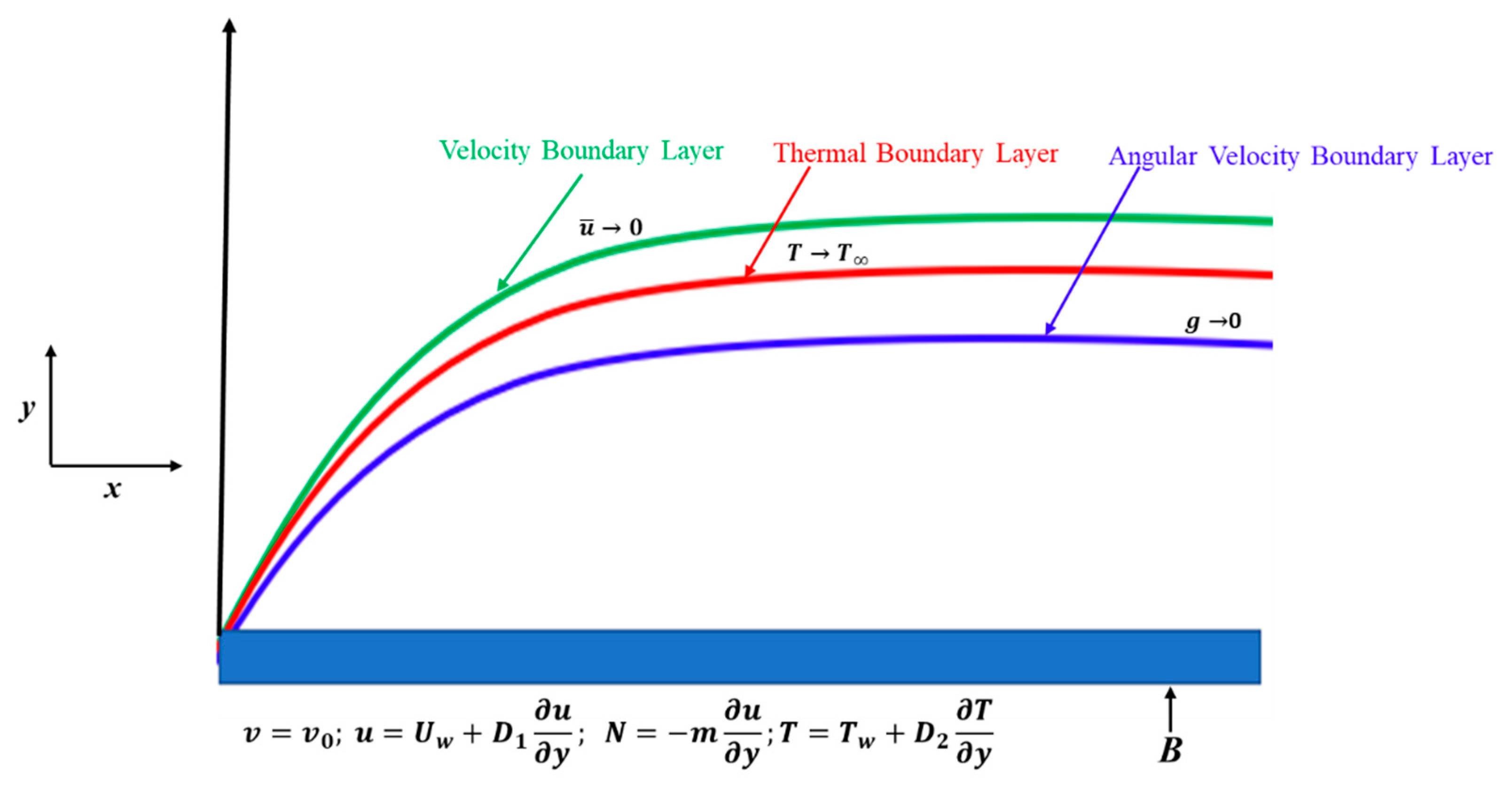
2. Problem Formulation

We considered MHD flow of micropolar fluid over the vertical shrinking surface at y = 0 . In addition, it is supposed that the velocity of a linear surface is U w = a x and the temperature distribution of the sheet is T w ( x ) = T + T 0   x 2 where T is the outside temperature of thermal boundary layer. A non-uniform magnetic field B [ 0 ,   B 0 ,   0 ] is applied normal to the surface. We neglect the induced magnetic field by considering low magnetic Reynolds number. Moreover, the effect of the electric filed is not present (refer to Figure 1 for details). Along with all mentioned conditions the governing problems can be expressed in vector form as follows:
Now, Equations (1)–(4) can be written in the boundary layer form for steady flow as follows:
  ·    V = 0
ρ d V d t = P + ( μ + κ ) 2 V + κ ( × N ) + ( J × B )
ρ j d N d t = γ 2 N κ ( 2 N × V )
ρ c p d T d t = k 1 2 T · q r + ( μ + κ ) Φ
where t is the time, V = [ u ¯ ( x , y ) , v ¯ ( x , y ) ] is the velocity vector, ρ = ρ ( x , t ) is the fluid density, μ is the dynamic viscosity of fluid, P is the pressure, = x ¯ i + y ¯ j is del or gradient operator, 2 = 2 x 2 ¯ + 2 y 2 ¯ is the Laplacian operator, T = T ¯ ( x , y ) is the temperature, J × B = σ B 0 2 V is the Lorentz force where B denotes the total magnetic field which is the sum of applied magnetic field B 0 and the induced magnetic field b , J represents the current density, N the micromotional or angular velocity, γ = ( μ + κ 2 )   j is the spin gradient viscosity, j is the gyration parameter of fluid, κ is the vortex viscosity. Moreover, q r shows the Rosseland approximation which can be defined as q r = 4 σ 1 3 k * [ T 4 x , T 4 y ] . Further, Φ = 2 [ ( u ¯ x ¯ ) 2 + ( v ¯ y ¯ ) 2 ] + ( v ¯ x ¯ + u ¯ y ¯ ) 2 is the dissipation function:
u x + v y = 0
u   u x   +   v   u y = ( ϑ + κ ρ ) 2 u y 2 + κ ρ N y σ * B 2 u ρ
u N x + v N y = 1 ρ j [ γ 2 N y 2 κ ( 2 N + u y ) ]
u   T x   +   v   T y   = ( k 1 ρ c p + 16 σ 1 T 3 3 k * ρ c p )   2 T y 2 + ( μ + κ ρ c p ) ( u y ) 2
whose associated boundary conditions are:
v = v 0 ;   u = U w + D 1 u y ;    N = m u y ;    T = T w + D 2 T y     a t      y = 0 u 0 ;   N 0 ;    T T ;      as    y
Here respective velocities of x-axis and y-axis are u and v , ϑ is the kinematic viscosity, k 1 is the thermal conductivity, σ * is the electrical conductivity, σ 1 is the Stefan-Boltzmann constant, k * is the mean absorption coefficient, m is the boundary parameter, c p is the specific heat at constant pressure, v 0 is the mass transfer velocity of the porous sheet, while D 1 and D 2 are the respective slip factors of velocity and temperature.
Following similarity variables are used to convert the PDEs into ODEs:
( = y a ϑ , u = a x f ( η ) , v = a ϑ f ( η ) , N = a ϑ a x g ( η ) , θ ( η ) = ( T T ) ( T w   T )  
By using of Equation (10) in Equations (5)–(9), we obtain:
( 1 + K ) f + f f f 2 + K g M f = 0   
( 1 + K 2 )   g + f g g f 2 K g K f = 0
1 P r ( 1 + 4 3 R d ) θ + f θ 2 f θ + E c ( 1 + K ) f 2 = 0
with boundary conditions:
f ( 0 ) = S ,   f ( 0 ) = 1 + α f ( 0 ) ,   g ( 0 ) = m f ( 0 ) , θ ( 0 ) = 1 + β θ ( 0 )   f ( η ) 0 ;   g ( η ) 0 ;   θ ( η ) 0 ;   a s   η
where differentiation with respect to η is denoted by prime, K = κ μ , M = σ * B 0 2 ρ a , P r = μ c p k 1 ,   R d = 4 T 3 σ 1 k 1 k * ,   E c = a 2 T 0 c p   , S = v w a ϑ , α = D 1 a ϑ   ,   β = D 2 a ϑ are micropolar parameter, Hartmann number, Prandtl number, thermal radiation parameter, Eckert number, suction/blowing parameter, velocity slip parameter, and thermal slip parameter, respectively. It is worth noting that strong concentration can be observed when m = 0 which means that microelements are unable to rotate. Further, weak concentration can be examined when m = 0 .5 which indicates that antisymmetric part of the stress tensor is vanishing. Similarly, m = 1 shows the turbulent flow model of boundary layer.
The physical quantities of interest are skin friction coefficient C f with surface shear stress τ w and local Nusselt number N u with surface heat flux q w are given by:
C f = 2 τ w ρ u w 2 ,   where   τ w = [ ( μ + κ ) u y + κ N ] y = 0 N u = x q w k 1 ( T w   T ) ,     q w = k 1 [ ( 1 + 16 σ * T 3 3 k 1 k * ) T y ] y = 0
Using Equation (10) in Equation (15), yields:
C f ( R e x ) 1 2 = ( 1 + ( 1 m ) K ) f ( 0 ) N u ( R e x ) 1 2 = ( 1 + 4 3 R d ) θ ( 0 )
where R e x = a x 2 / ϑ is local Reynolds number.

3. Stability Analysis

According to Weidman et al. [49] and Lund et al. [50], the existence of multiple solutions is possible in fluid flow problems in some ranges of physical parameters. It is necessary to carry out stability analysis in order to determine which one solution is stable. For this purpose, a new dimensionless time variable τ   =   a t is presented to model the problem. Dimensionless similarity variables in terms of τ can be expressed as follows:
η = y a ϑ , τ   =   a t ,   u = a x f ( η , τ ) , v = a ϑ f ( η , τ ) , N = a ϑ a x g ( η , τ ) , θ ( η , τ ) = ( T T ) ( T w   T )
As a result, Equations (6)–(8) are written as follows:
u t   + u   u x   +   v   u y = ( ϑ + κ ρ ) 2 u y 2 + κ ρ N y σ * B 2 u ρ  
N t + u N x + v N y = 1 ρ j [ γ 2 N y 2 κ ( 2 N + u y ) ]
T t + u   T x   +   v   T y   = ( k 1 ρ c p + 16 σ * T 3 3 k * ρ c p )   2 T y 2 + ( μ + κ ρ c p ) ( u y ) 2
Substituting Equation (17) in Equations (18)–(20), we have:
( 1 + K ) 3 f η 3 + f 2 f η 2 ( f η ) 2 + K g η M f η 2 f τ η = 0
( 1 + K 2 )   2 g η 2 + f g η g f η 2 K g K 2 f η 2 g τ = 0
1 P r ( 1 + 4 3 R d ) 2 θ η 2 + f θ η 2 θ f η + E c ( 1 + K ) 2 f η 2 θ τ = 0
subject to boundary conditions:
f ( 0 , τ ) = S ;   f ( 0 ,   τ ) η = 1 + α 2 f ( 0 ,   τ ) η 2   and   f ( η ,   τ ) η 0   as   η   h ( 0 , τ ) = m 2 f ( 0 ,   τ ) η 2   and   h ( η , τ ) 0   as   η θ ( 0 , τ ) = 1 + β   θ ( 0 , τ ) η   and   θ ( η , τ ) 0    as   η
The steady flow solutions ( f ( η ) = f 0 ( η ) , g ( η ) = g 0 ( η ) , θ ( η ) = θ 0 ( η ) ) must satisfy the corresponding boundary conditions in order to perform the solution’s stability. The complete functions of solution are expressed as:
f ( η , τ ) = f 0 ( η ) + e ε τ F ( η , τ ) g ( η , τ ) = g 0 ( η ) + e ε τ H ( η , τ ) θ ( η , τ ) = θ 0 ( η ) + e ε τ G ( η , τ )
where F ( η , τ ) , H ( η , τ ) , and G ( η , τ ) are small relative to f 0 ( η ) , g 0 ( η ) , and θ 0 ( η ) respectively and ε is the unknow eigenvalue. By using Equation (23) in Equations (21)–(24) and by keeping τ = 0 (the steady state), we get the linearized form of the equations:
( 1 + K ) F 0 + f 0 F 0 + F 0 f 0 2 f 0 F 0 + K H 0 M F 0 + ε F 0 = 0  
( 1 + K 2 ) H 0 + f 0 H 0 + F 0 g 0 g 0 F 0 g 0 F 0 2 K H 0 K F 0 + ε H 0 = 0
1 P r ( 1 + 4 3 R d ) G 0 + f 0 G 0 + F 0 θ 0 2 f 0 G 0 2 F 0 θ 0 + 2 E c .   ( 1 + K ) f 0 F 0 + ε G 0 = 0
with the boundary conditions:
F 0 ( 0 ) = 0 ,        F 0 ( 0 ) = α F 0 ( 0 ) ,      H 0 ( 0 ) = m F 0 ( 0 ) ,      G 0 ( 0 ) = β   G 0 ( 0 ) F 0 ( η ) 0 ,     G 0 ( η ) 0 ,         H 0 ( η ) 0    as    η
The stability of the steady solution has been studied by finding the values of smallest eigenvalue. According to Haris et al. [51] and Ali et al. [52], we need to relax the condition in order to determine the range of possible eigenvalues. For current problem, F 0 ( η ) 0 as η is relaxed to F 0 ( 0 ) = 1 .

4. Numerical Method

When the system of ODEs is non-linear then it is not possible to find the solution of the system in an exact form of solution. Henceforth, we look to the numerical approach. In this paper, the shooting method has been used to solve the system of non-linear ODEs with boundary conditions. The shooting method converts the boundary conditions into initial conditions and a higher order of ODEs to first-order ODEs. The resultant system of first-order ODEs has been solved by the Runge-Kutta 4th order method. The detail of the present method is as follows:
p = f , q =   p ,   p 1 = g ;   ( 1 + K ) q = p 2 f q K p 1 + M p
p 1 = g ;   ( 1 + K 2 ) p 1 = g p f p 1 2 K g K q   
r = θ ;   ( 1 + 4 3 R d ) r = P r { 2 p θ f r E c   ( 1 + K ) q 2 }
with conditions:
f ( 0 ) = S ;    p ( 0 ) = 1 + α q ( 0 ) ;   q ( 0 ) = α 1 g ( 0 ) = m α 1 ;   p 1 ( 0 ) = α 2   θ ( 0 ) = 1 + β r ( 0 ) ; r ( 0 ) = α 3
where unknown initial conditions are denoted by α 1 , α 2 and α 3 . It is worth mentioning that the missing initial values of α 1 , α 2 and α 3 are needed to shoot such that profiles of the solutions satisfy the original boundary conditions which are f ( η ) 0 ;   g ( η ) 0 ;   and   θ ( η ) 0   as   η .

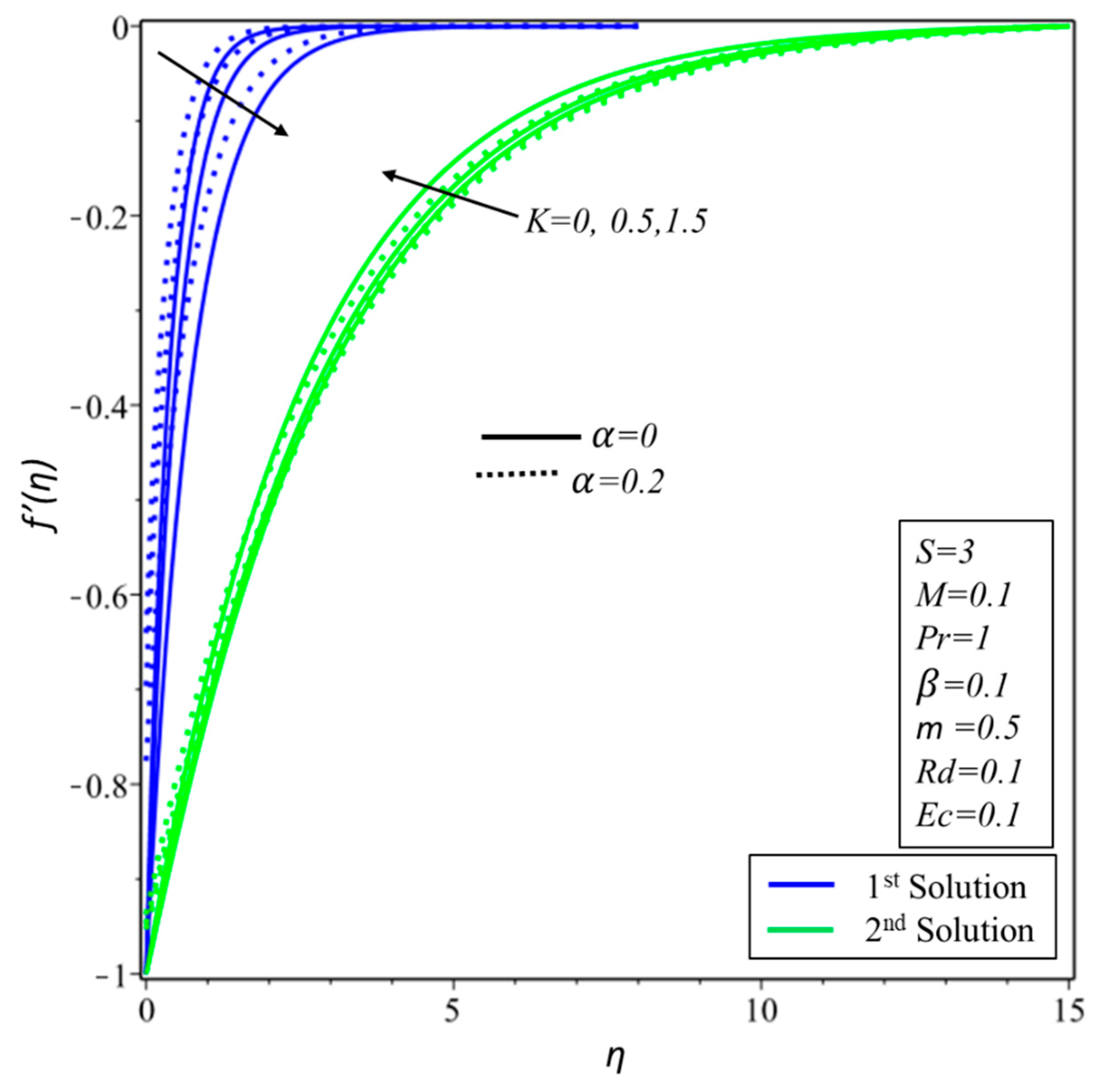
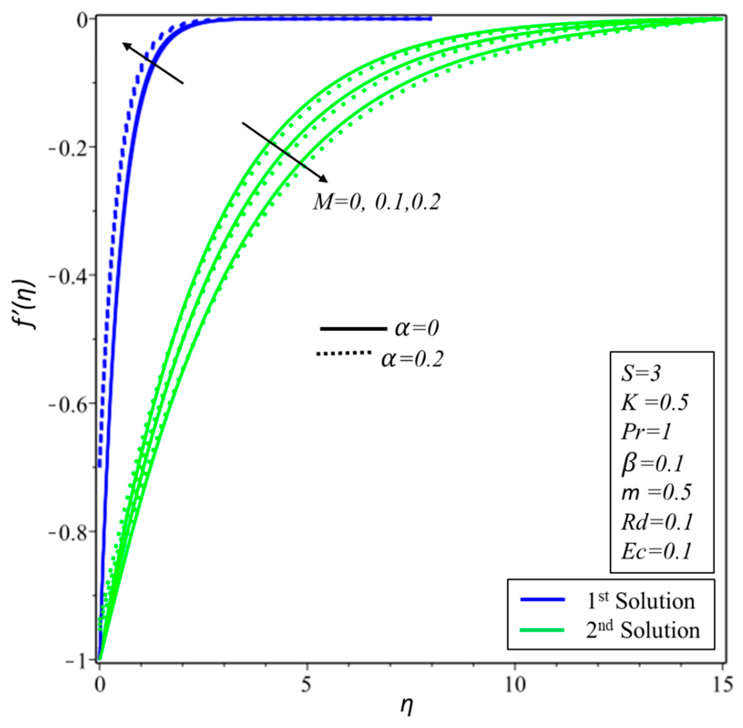
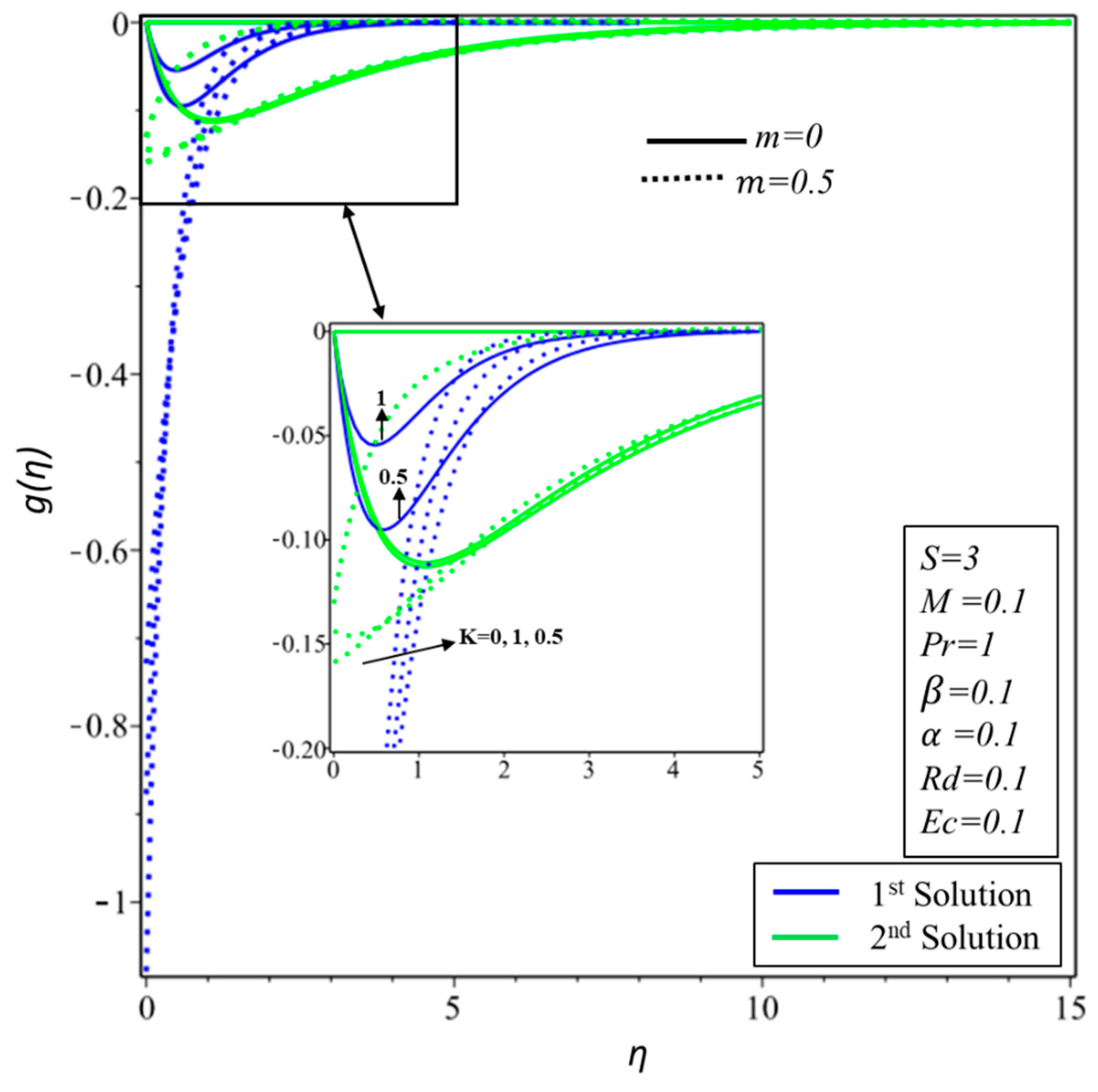
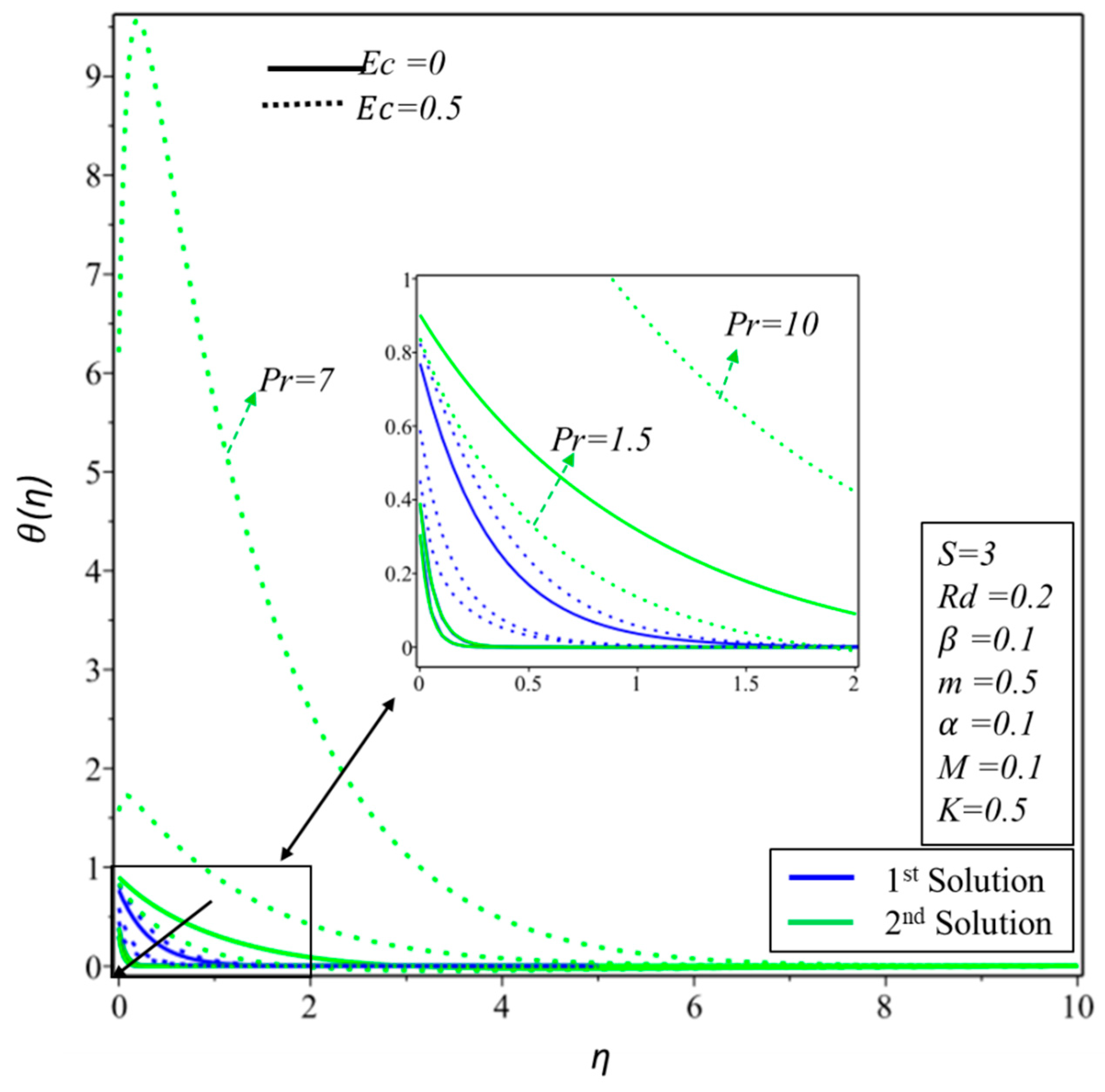
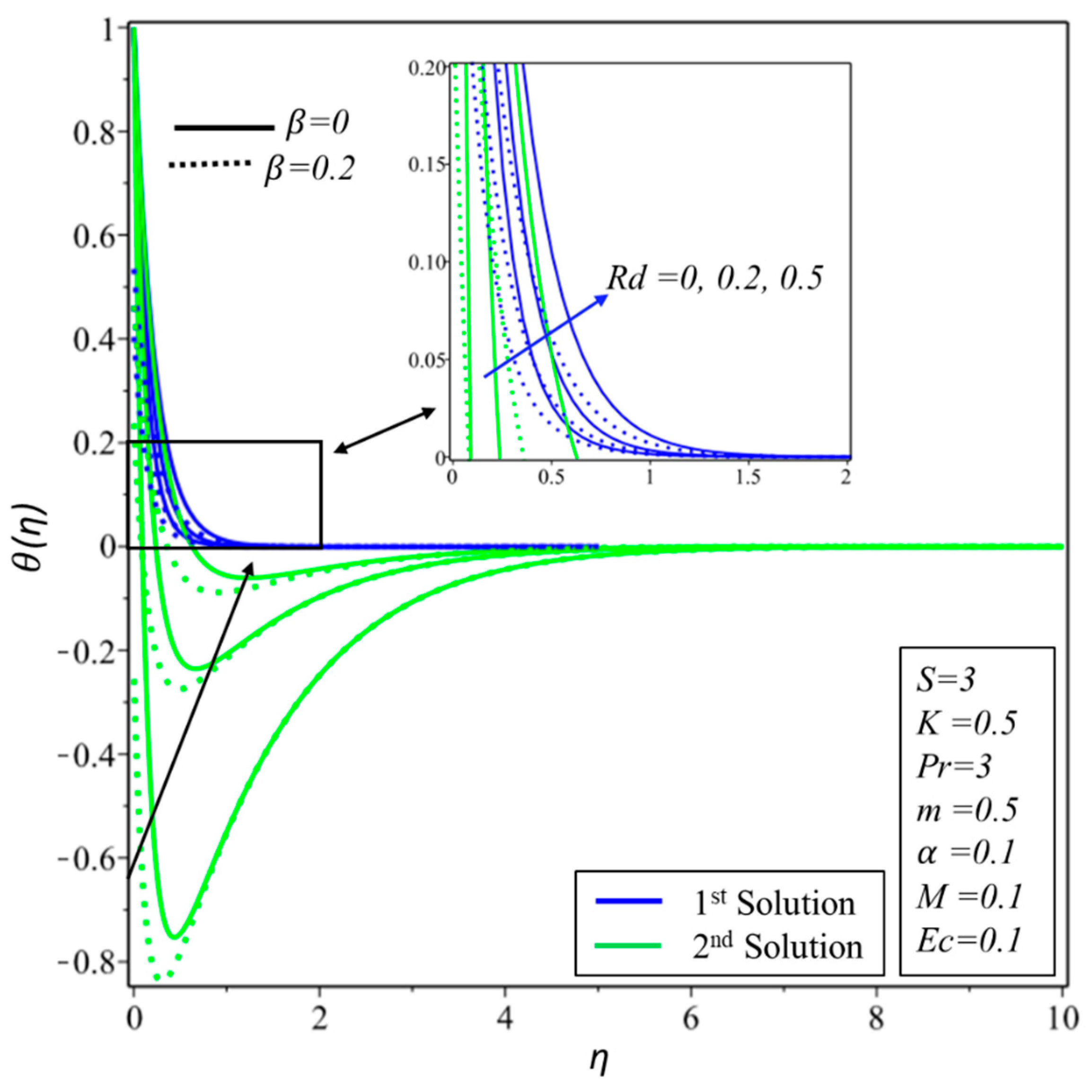
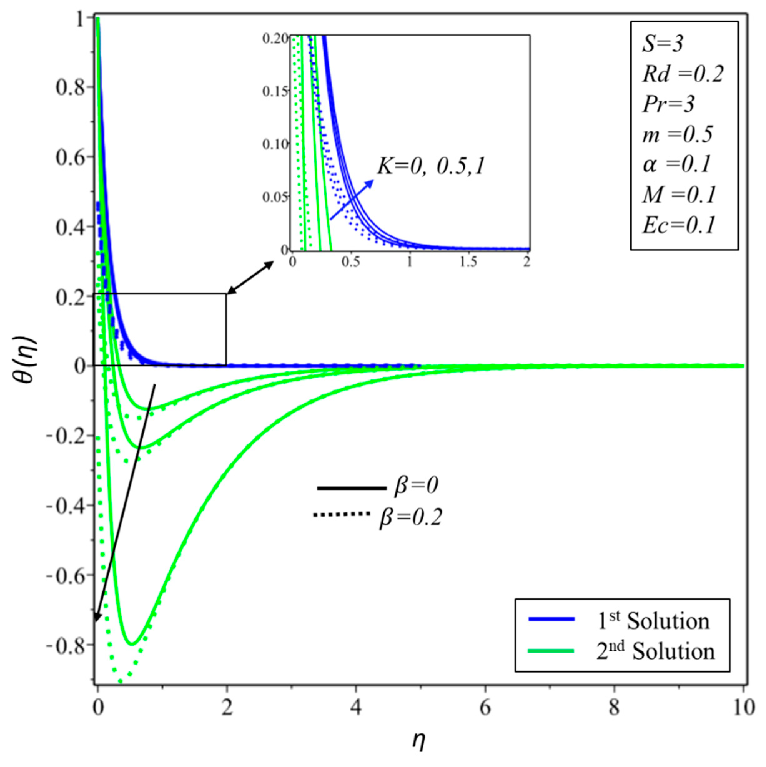
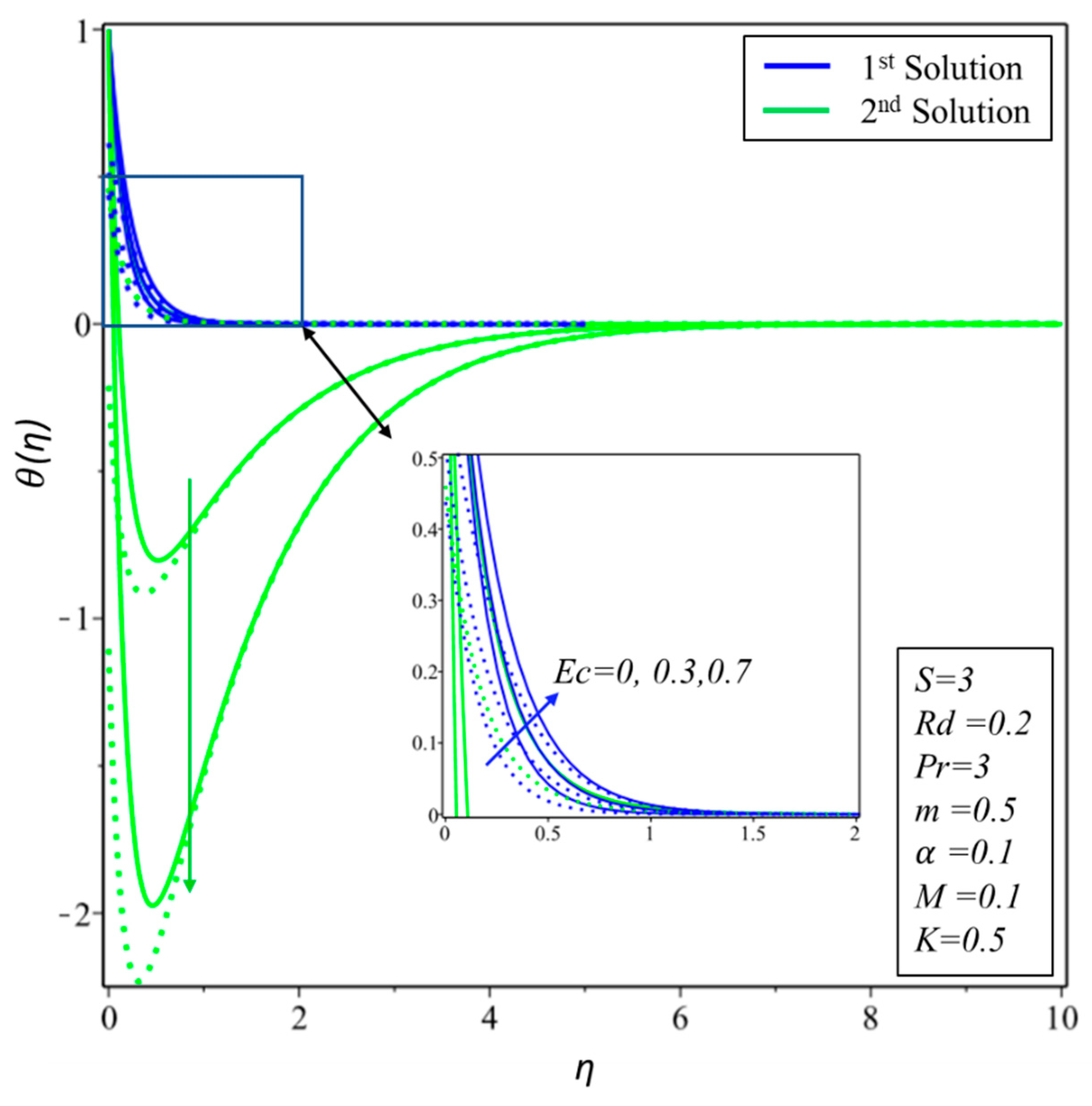
5. Results and Discussion

Steady MHD flow of electrically conducted micropolar fluid in the presence of viscous dissipation and thermal radiation have been examined. Moreover, the effect of velocity and thermal slip condition have also been taken into account. Shooting method with 4th order RK method has been employed with help of shootlib function in Maple 2018 to get the solutions of the governing non-linear ODEs as stated in Equations (11)–(13). The numerical results revealed that dual solutions exist for different ranges of applied parameters. In addition, the system of governing Equations (26)–(28) with boundary condition (29) has been solved by employing the BVP4C package presented in MATLAB in order to perform the stability analysis of solutions. BVP4C package is created on the finite difference scheme by applying three-stage Lobatto IIIa formula possessing fourth-order accuracy. A good initial guess is important to predict the existence of the dual solution. Normally, fix numbers are kept for the first solution (it is always not necessary), while the second solution depends upon the good initial guesses. These good guesses should satisfy the boundary conditions and fulfill boundary conditions asymptotically. Further, if any guess fails to generate the convergent solution then an appropriate set of values of parameters are needed to be selected using trial approach in order to make appropriate guesses for finding the second solution. The results of the smallest eigenvalue are given in Table 1. It can be seen that the signs of the smallest eigenvalue for the first (second) solution are positive (negative) which mean that first (second) solution is stable (unstable). In order to validate our numerical results, we compared the values of skin friction coefficient with the exact solutions of Equation (11). As shown in Table 2, both results were found in excellent agreement with maximum absolute errors of the stable (unstable) solution is 10 5 ( 10 3 ). It worth to mention that if α = M = 0 and m = 0.5 , Equation (11) is reduced to f ( η ) = S 1 e λ η λ which implies that f ( 0 ) = S ± S 2 2 K 4 ( 2 + K ) (refer to [37]). The dimensionless coupled linear boundary layer ODEs have been solved for velocity, micro-rotation, and temperature profiles with the impact of the emerging micropolar parameter, Hartmann number, Prandtl number, thermal radiation parameter, Eckert number, Suction/Blowing parameter, velocity slip parameter, and thermal slip parameter.
Figure 2 exhibits the velocity profile ( f ( η ) ) with the effect of material parameter ( K ). The fluid velocity increases as values of K get higher and hence the boundary layer thickness becomes thicker in the first solution. On the other hand, reverse behavior of velocity of fluid has been noticed in the second solution. This decreasing behavior is caused by the created resistance of micropolar parameter on the velocity field which reduces the fluid velocity. The velocity distribution, displayed in Figure 2, reveals that the motion rate is significantly increases for the no-slip condition. It is also observed that the thickness of momentum boundary layer reduces as the increase of velocity slip parameter as compared to α = 0 in both solutions. Figure 3 depicts the profile of velocity ( f ( η ) ) for several values of M . The fluid velocity increases for the strong effect of the magnetic field in the second solution. However, the velocity and thickness of the momentum boundary layer tend to decrease in the first solution as expected. Physically, the magnetic force called a Lorentz force creates the intense drag force which resists the flow of fluid. Thus, the fluid velocity and hydrodynamic boundary layer thickness are reduced. The variation of material parameter ( K ) on the micro-rotation profile ( g ( η ) ) is revealed in Figure 4. For the first solution when m = 0 ,   1 the micro-rotation profile rises in the range 0 K 0.5 and decreases in the range 0.5 < K 1 . On the other hand, same behavior is noted for the second solution as noticed in the first solution.
The graph of the temperature profile ( θ ( η ) ) in the presence and absence of Eckert number ( E c ) for various values of Prandtl number ( P r ) is drawn in Figure 5. Temperature of the fluid is noticed to reduce when P r increases in both solutions. Physically, the enhancement in the effect of the Prandtl number reduces the thermal diffusivity which causes the reduction in the thermal boundary layer thickness. Therefore, it can be concluded that the Prandtl number controls the thickness of thermal boundary layer and cooling in conducting flows. In the case of small Prandtl number, heat spreads quickly from the surface to the fluid flow which implies that the thickness of thermal boundary layer is much higher for the liquid metals, i.e., range of Prandtl number for liquid metals is 0.01 to 0.001. The interesting behavior is noticed for the second solution when E c = 0 where the thickness of thermal boundary layer increases when 1.5 P r 7 and decreases when 7 < P r 10 . Figure 6 demonstrates the behavior of temperature profiles ( θ ( η ) ) for increasing values of the thermal radiation ( R d ). It is detected that the thickness of thermal boundary layer and temperature increase when thermal radiation parameter is increased in both solutions. This agrees with the physical fact that thermal radiation spreads heat from surface to fluid flow and consequently the thermal boundary layer becomes thicker. The situation can also be further explained by relationship between the Prandtl number and thermal radiation parameter given by 1 P r ( 1 + 4 3 R d ) . It can be clearly seen that if the values of R d increase then the effect of thermal diffusivity increases. On the other hand, when the value of P r decreases, the thickness of thermal boundary and temperature of fluid increase.
The temperature distributions ( θ ( η ) ) for various values of K in presence and absence of thermal slip effect is shown in Figure 7. It is reckoned that the thickness of the thermal boundary layer tends to increase for the higher effect of the material parameter in the first solution. On the other hand, the reverse trend of temperature is found in the second solution. It is worth to notice that all plots (2–8) satisfy asymptotically the far-field boundary conditions for both solutions which show the validity of the shooting methods and generated numerical results. The variation of Eckert number on the non-dimensional fluid temperature profiles is revealed in Figure 8, indicating that both temperature and thickness of thermal boundary layer increase in the first solution. This increment of temperature is caused by smaller effect of enthalpy difference of boundary layer since Eckert number is the ratio of the kinetic energy flow and an enthalpy difference of boundary layer. Eckert number helps the converting of kinetic energy into internal energy by opposing fluid stresses. It is worth mentioning that the loss of temperature from the surface to the fluid flow is possible for 0 < E c 1 . On the other hand, the opposite behavior of temperature profiles is examined.
It can be easily seen from Figure 9, Figure 10 and Figure 11 that multiple solutions exist for different ranges of S which depend upon the values of the material parameter. From those figures, we observed that dual solutions exist for S S c i , i = 0 ,   1 ,   2 and no solution exists when S < S c i where S c i is the critical values of S when dual solutions occur. The variation of critical values totally depends upon the values of K . Variation of skin friction coefficient ( f ( 0 ) ) with respect to K for different values of S is demonstrated in Figure 9. It can be examined easily that increments in suction produce more drag forces as compared to the material parameter ( K ) in the first solution. As a result, skin friction increases in the first solution. On contrary, the opposite trend is noticed for the second solution. The same behavior of couple stress coefficient ( g ( 0 ) ) is examined in Figure 11 which we noticed for the skin friction coefficient in both solutions. The effect of suction and material parameter ( K ) on the heat transfer rate ( θ ( 0 ) ) was drawn in Figure 10. There exists discontinuity in the second solution which indicate instability of the solution. Finally, it is also noticed that the heat transfer rate is lower for the higher values of material parameters in the first solutions. Moreover, the increasing of the suction would reason the rate of heat transfer to accelerate because the temperature is simply diffused over the permeable sheet relatively than an impenetrable sheet.

6. Conclusions

Studies on a micropolar fluid considering the effects of thermal radiation, velocity slip, thermal slip and viscous dissipation have been carried out to investigate the existence of all possible multiple solutions. Mathematical formulations of the micropolar problem has been gotten by employing the fundamental laws of conservations. The governing equations are transformed to equations of boundary layers. The highly non-linear coupled partial differential equations (PDEs) are then converted into non-dimensional ordinary differential equations (ODEs) by using of linear transformations. Some important outcomes of this study can be summarized as follows:
(1)
Dual solutions exist over the permeable shrinking sheet and the critical values S c of suction parameter depends on material parameter K .
(2)
Velocity field and the thickness of hydrodynamic boundary layer increase (decrease) in the first solution and decrease (increases) in the second solution when K ( M ) is increased.
(3)
Both solutions increase (decrease) for the strong effect of E c and R d ( P r ).
(4)
The material parameter and mass suction parameter are inversely proportional to each other’s.
(5)
The results of numerical solutions are closed to the exact solutions.
(6)
The results of the smallest eigenvalues show that second solution is not stable as compared to the first solution.
(7)
The realizable flow situation is only possible for the first solution.

Author Contributions

L.A.L. derived the equations and generated the results and wrote the paper. Z.O. formulated the model and proof read the manuscript. I.K. checked the whole manuscript. S.K. derived the equations of stability analysis. S.R. wrote the introduction section. I.A.M. performed the stability analysis. K.S.N. wrote the paper and checked the manuscript.

Funding

This work was supported by the National Research Foundation of Korea(NRF) grant funded by the Korea government(MSIT) (No. 2019M3F2A1073179). This research is also supported by the Univeristi Utara Malaysia.

Acknowledgments

The authors gratefully acknowledge the financial support of National Research Foundation of Korea(NRF) grant funded by the Korea government(MSIT) (No. 2019M3F2A1073179. The first author is thankful to Sindh Agriculture University Tandojam for granting the study leave.

Conflicts of Interest

The authors declare no conflict of interest.

Nomenclature

T   0 a constant
T ambient temperature
N angular velocity
J current density
Φ dissipation function
μ dynamic viscosity
E c Eckert number
σ * electrical conductivity
gradient operator
j gyration parameter
M Hartmann number
2 Laplacian operator
N u local Nusselt number
R e local Reynolds number
J × B Lorentz force
B Magnetic field vector
v 0 mass transfer velocity
k * mean absorption coefficient,
K Positive constant
P r Prandtl number
P pressure
q r Rosseland approximation
C f skin friction coefficient
D 2 slip factors of temperature
D 1 slip factors of velocity
ε smallest eigen value
γ spin gradient viscosity
τ Stability transformed variable
σ 1 Stefan-Boltzmann constant
TTemperature
R d thermal radiation
β thermal slip parameter
t time
η transformed variable
T w ( x ) variable temperature of surface
u, vvelocity components
U w Velocity of shrinking surface
α velocity slip parameter
V Velocity vector
κ vortex viscosity

References

  1. Dero, S.; Rohni, A.M.; Saaban, A. MHD micropolar nanofluid flow over an exponentially stretching/shrinking surface: Triple solutions. J. Adv. Res. Fluid Mech. Therm. Sci 2019, 56, 165–174. [Google Scholar]
  2. Hayat, T.; Khan, M.I.; Waqas, M.; Alsaedi, A.; Khan, M.I. Radiative flow of micropolar nanofluid accounting thermophoresis and Brownian moment. Int. J. Hydrog. Energy 2017, 42, 16821–16833. [Google Scholar] [CrossRef]
  3. Zubair, M.; Shah, Z.; Dawar, A.; Islam, S.; Kumam, P.; Khan, A. Entropy generation optimization in squeezing magnetohydrodynamics flow of casson nanofluid with viscous dissipation and joule heating effect. Entropy 2019, 21, 747. [Google Scholar] [CrossRef] [Green Version]
  4. Qing, J.; Bhatti, M.; Abbas, M.; Rashidi, M.; Ali, M. Entropy generation on MHD Casson nanofluid flow over a porous stretching/shrinking surface. Entropy 2016, 18, 123. [Google Scholar] [CrossRef]
  5. Aurangzaib Bhattacharyya, K.; Shafie, S. Effect of partial slip on an unsteady MHD mixed convection stagnation-point flow of a micropolar fluid towards a permeable shrinking sheet. Alex. Eng. J. 2016, 55, 1285–1293. [Google Scholar] [CrossRef] [Green Version]
  6. OAlzahrani, E.; Shah, Z.; Alghamdi, W.; Zaka Ullah, M. Darcy–Forchheimer Radiative Flow of Micropoler CNT Nanofluid in Rotating Frame with Convective Heat Generation/Consumption. Processes 2019, 7, 666. [Google Scholar] [CrossRef] [Green Version]
  7. Omori, T.; Ishikawa, T. Swimming of Spermatozoa in a Maxwell Fluid. Micromachines 2019, 10, 78. [Google Scholar] [CrossRef] [Green Version]
  8. Zafar, M.; Ahmad, B.; Rana, M.A.; Zahid, M. Mathematical Analysis of the Coating Process Over a Porous Web Lubricated with Upper Convected Maxwell Fluid. Coatings 2019, 9, 458. [Google Scholar] [CrossRef] [Green Version]
  9. Guo, X.; Qi, H. Analytical solution of electro-osmotic peristalsis of fractional Jeffreys fluid in a micro-channel. Micromachines 2017, 8, 341. [Google Scholar] [CrossRef] [Green Version]
  10. Hayat, T.; Qayyum, S.; Imtiaz, M.; Alsaedi, A. Impact of Cattaneo-Christov heat flux in Jeffrey fluid flow with homogeneous-heterogeneous reactions. PLoS ONE 2016, 11, e0148662. [Google Scholar] [CrossRef]
  11. Khan, W.A.; Irfan, M.; Khan, M.; Alshomrani, A.S.; Alzahrani, A.K.; Alghamdi, M.S. Impact of chemical processes on magneto nanoparticle for the generalized Burgers fluid. J. Mol. Liq. 2017, 234, 201–208. [Google Scholar] [CrossRef]
  12. Maleki, H.; Safaei, M.R.; Togun, H.; Dahari, M. Heat transfer and fluid flow of pseudo-plastic nanofluid over a moving permeable plate with viscous dissipation and heat absorption/generation. J. Therm. Anal. Calorim. 2019, 135, 1643–1654. [Google Scholar] [CrossRef]
  13. Eringen, A.C. Theory of micropolar fluids. J. Math. Mech. 1966, 16, 1–18. [Google Scholar] [CrossRef]
  14. Bhattacharjee, B.; Chakraborti, P.; Choudhuri, K. Evaluation of the performance characteristics of double-layered porous micropolar fluid lubricated journal bearing. Tribol. Int. 2019. [Google Scholar] [CrossRef]
  15. Koriko, O.K.; Animasaun, I.L.; Omowaye, A.J.; Oreyeni, T. The combined influence of nonlinear thermal radiation and thermal stratification on the dynamics of micropolar fluid along a vertical surface. Multidiscip. Modeling Mater. Struct. 2019, 15, 133–155. [Google Scholar] [CrossRef]
  16. Lakshmi, R.V.; Sarojamma, G.; Sreelakshmi, K.; Vajravelu, K. Heat Transfer Analysis in a Micropolar Fluid with Non-Linear Thermal Radiation and Second-Order Velocity Slip. In Applied Mathematics and Scientific Computing; Birkhäuser: Cham, Switzerland, 2019; pp. 385–395. [Google Scholar]
  17. Mozaffari, M.; D’Orazio, A.; Karimipour, A.; Abdollahi, A.; Safaei, M.R. Lattice Boltzmann method to simulate convection heat transfer in a microchannel under heat flux: Gravity and inclination angle on slip-velocity. Int. J. Numer. Methods Heat Fluid Flow 2019. [Google Scholar] [CrossRef]
  18. Khan, A.A.; Batool, R.; Kousar, N. MHD Micropolar Fluid over Curved Stretching Surface with modified Fourier law. Sci. Iran. 2019. [Google Scholar] [CrossRef] [Green Version]
  19. Maleki, H.; Safaei, M.R.; Alrashed, A.A.; Kasaeian, A. Flow and heat transfer in non-Newtonian nanofluids over porous surfaces. J. Therm. Anal. Calorim. 2019, 135, 1655–1666. [Google Scholar] [CrossRef]
  20. Gholamalizadeh, E.; Pahlevanzadeh, F.; Ghani, K.; Karimipour, A.; Nguyen, T.K.; Safaei, M.R. Simulation of water/FMWCNT nanofluid forced convection in a microchannel filled with porous material under slip velocity and temperature jump boundary conditions. Int. J. Numer. Methods Heat Fluid Flow 2019. [Google Scholar] [CrossRef]
  21. Nikkhah, Z.; Karimipour, A.; Safaei, M.R.; Forghani-Tehrani, P.; Goodarzi, M.; Dahari, M.; Wongwises, S. Forced convective heat transfer of water/functionalized multi-walled carbon nanotube nanofluids in a microchannel with oscillating heat flux and slip boundary condition. Int. Commun. Heat Mass Transf. 2015, 68, 69–77. [Google Scholar] [CrossRef]
  22. Abidi, A.; Raizah, Z.; Madiouli, J. Magnetic Field Effect on the Double Diffusive Natural Convection in Three-Dimensional Cavity Filled with Micropolar Nanofluid. Appl. Sci. 2018, 8, 2342. [Google Scholar] [CrossRef] [Green Version]
  23. Magodora, M.; Mondal, H.; Sibanda, P. Dual solutions of a micropolar nanofluid flow with radiative heat mass transfer over stretching/shrinking sheet using spectral quasilinearization method. Multidiscip. Modeling Mater. Struct. 2019. [Google Scholar] [CrossRef]
  24. Karimipour, A.; Nezhad, A.H.; D’Orazio, A.; Esfe, M.H.; Safaei, M.R.; Shirani, E. Simulation of copper–water nanofluid in a microchannel in slip flow regime using the lattice Boltzmann method. Eur. J. Mech. B Fluids 2015, 49, 89–99. [Google Scholar] [CrossRef]
  25. Zaib, A.; Haq, R.U. Magnetohydrodynamics mixed convective flow driven through a static wedge including TiO2 nanomaterial with micropolar liquid: Similarity dual solutions via finite difference method. Proc. Inst. Mech. Eng. Part C J. Mech. Eng. Sci. 2019. [Google Scholar] [CrossRef]
  26. Lund, L.A.; Omar, Z.; Dero, S.; Khan, I. Linear stability analysis of MHD flow of micropolar fluid with thermal radiation and convective boundary condition: Exact solution. Heat Transf. Asian Res. 2019, 1–16. [Google Scholar] [CrossRef]
  27. Ishak, A.; Nazar, R.; Pop, I. Magnetohydrodynamic (MHD) flow of a micropolar fluid towards a stagnation point on a vertical surface. Comput. Math. Appl. 2008, 56, 3188–3194. [Google Scholar] [CrossRef] [Green Version]
  28. Raza, J.; Rohni, A.M.; Omar, Z. Rheology of micropolar fluid in a channel with changing walls: Investigation of multiple solutions. J. Mol. Liq. 2016, 223, 890–902. [Google Scholar] [CrossRef]
  29. Lund, L.A.; Omar, Z.; Khan, I. Quadruple Solutions of Mixed Convection Flow of Magnetohydrodynamic Nanofluid Over Exponentially Vertical Shrinking and Stretching Surfaces: Stability Analysis. Comput. Methods Programs Biomed. 2019. [Google Scholar] [CrossRef]
  30. Schlichting, H. Boundary Layer Theory; McGraw-Hill Inc.: New York, NY, USA, 1979. [Google Scholar]
  31. Soid, S.K.; Ishak, A.; Pop, I. MHD flow and heat transfer over a radially stretching/shrinking disk. Chin. J. Phys. 2018, 56, 58–66. [Google Scholar] [CrossRef]
  32. Khan, M.; Irfan, M.; Ahmad, L.; Khan, W.A. Simultaneous investigation of MHD and convective phenomena on time-dependent flow of Carreau nanofluid with variable properties: Dual solutions. Phys. Lett. A 2018, 34, 2334–2342. [Google Scholar] [CrossRef]
  33. Raju, C.S.K.; Sandeep, N.; Babu, M.J.; Sugunamma, V. Dual solutions for three-dimensional MHD flow of a nanofluid over a nonlinearly permeable stretching sheet. Alex. Eng. J. 2016, 55, 151–162. [Google Scholar] [CrossRef] [Green Version]
  34. Lok, Y.Y.; Ishak, A.; Pop, I. Oblique stagnation slip flow of a micropolar fluid towards a stretching/shrinking surface: A stability analysis. Chin. J. Phys. 2018, 56, 3062–3072. [Google Scholar] [CrossRef]
  35. Sandeep, N.; Sulochana, C. Dual solutions for unsteady mixed convection flow of MHD micropolar fluid over a stretching/shrinking sheet with non-uniform heat source/sink. Eng. Sci. Technol. Int. J. 2015, 18, 738–745. [Google Scholar] [CrossRef] [Green Version]
  36. Yacob, N.A.; Ishak, A.; Pop, I. Melting heat transfer in boundary layer stagnation-point flow towards a stretching/shrinking sheet in a micropolar fluid. Comput. Fluids 2011, 47, 16–21. [Google Scholar] [CrossRef]
  37. Turkyilmazoglu, M. A note on micropolar fluid flow and heat transfer over a porous shrinking sheet. Int. J. Heat Mass Transf. 2014, 72, 388–391. [Google Scholar] [CrossRef]
  38. Bhattacharyya, K.; Mukhopadhyay, S.; Layek, G.C.; Pop, I. Effects of thermal radiation on micropolar fluid flow and heat transfer over a porous shrinking sheet. Int. J. Heat Mass Transf. 2012, 55, 2945–2952. [Google Scholar] [CrossRef]
  39. Wilks, G.; Bramley, J.S. Dual solutions in mixed convection. Proc. R. Soc. Edinb. Sect. A Math. 1981, 87, 349–358. [Google Scholar] [CrossRef]
  40. Merkin, J.H. On dual solutions occurring in mixed convection in a porous medium. J. Eng. Math. 1986, 20, 171–179. [Google Scholar] [CrossRef]
  41. Ali, F.M.; Naganthran, K.; Nazar, R.; Pop, I. MHD mixed convection boundary layer stagnation-point flow on a vertical surface with induced magnetic field. Int. J. Numer. Methods Heat Fluid Flow 2019. [Google Scholar] [CrossRef]
  42. Lund, L.A.; Omar, Z.; Khan, I. Analysis of dual solution for MHD flow of Williamson fluid with slippage. Heliyon 2019, 5, e01345. [Google Scholar] [CrossRef] [Green Version]
  43. Khan, M.; Alshomrani, A.S.; Haq, R.U. Investigation of dual solutions in flow of a non-Newtonian fluid with homogeneous–heterogeneous reactions: Critical points. Eur. J. Mech. B Fluids 2018, 68, 30–38. [Google Scholar]
  44. Jusoh, R.; Nazar, R.; Pop, I. Impact of heat generation/absorption on the unsteady magnetohydrodynamic stagnation point flow and heat transfer of nanofluids. Int. J. Numer. Methods Heat Fluid Flow 2019. [Google Scholar] [CrossRef]
  45. Lund, L.A.; Ching, D.L.C.; Omar, Z.; Khan, I.; Nisar, K.S. Triple Local Similarity Solutions of Darcy-Forchheimer Magnetohydrodynamic (MHD) Flow of Micropolar Nanofluid Over an Exponential Shrinking Surface: Stability Analysis. Coatings 2019, 9, 527. [Google Scholar] [CrossRef] [Green Version]
  46. Khan, Z.H.; Qasim, M.; Haq, R.U.; Al-Mdallal, Q.M. Closed form dual nature solutions of fluid flow and heat transfer over a stretching/shrinking sheet in a porous medium. Chin. J. Phys. 2017, 55, 1284–1293. [Google Scholar] [CrossRef]
  47. Raza, J.; Rohni, A.M.; Omar, Z.; Awais, M. Heat and mass transfer analysis of MHD nanofluid flow in a rotating channel with slip effects. J. Mol. Liq. 2016, 219, 703–708. [Google Scholar] [CrossRef]
  48. Rohni, A.M.; Ahmad, S.; Pop, I. Flow and heat transfer at a stagnation-point over an exponentially shrinking vertical sheet with suction. Int. J. Therm. Sci. 2014, 75, 164–170. [Google Scholar] [CrossRef]
  49. Weidman, P.D.; Kubitschek, D.G.; Davis, A.M.J. The effect of transpiration on self-similar boundary layer flow over moving surfaces. Int. J. Eng. Sci. 2006, 44, 730–737. [Google Scholar] [CrossRef]
  50. Lund, L.A.; Omar, Z.; Khan, I. Steady incompressible magnetohydrodynamics Casson boundary layer flow past a permeable vertical and exponentially shrinking sheet: A stability analysis. Heat Transf. Asian Res. 2019. [Google Scholar] [CrossRef]
  51. Harris, S.D.; Ingham, D.B.; Pop, I. Mixed convection boundary-layer flow near the stagnation point on a vertical surface in a porous medium: Brinkman model with slip. Transp. Porous Media 2009, 77, 267–285. [Google Scholar] [CrossRef]
  52. Ali, L.L.; Omar, Z.; Khan, I.; Raza, J.; Bakouri, M.; Tlili, I. Stability Analysis of Darcy-Forchheimer Flow of Casson Type Nanofluid Over an Exponential Sheet: Investigation of Critical Points. Symmetry 2019, 11, 412. [Google Scholar]
Figure 1. Schematic diagram.
Energies 12 04617 g001
Figure 2. The velocity profiles f ( η ) for various values of K .
Energies 12 04617 g002
Figure 3. The velocity profiles f ( η ) for various values of M .
Energies 12 04617 g003
Figure 4. The Microrotation profiles g ( η ) for various values of K .
Energies 12 04617 g004
Figure 5. The temperature profiles θ(η) for various values of Pr.
Energies 12 04617 g005
Figure 6. The temperature profiles θ(η) for various values of Rd.
Energies 12 04617 g006
Figure 7. The temperature profiles θ(η) for various values of K.
Energies 12 04617 g007
Figure 8. The temperature profiles θ(η) for various values of Ec.
Energies 12 04617 g008
Figure 9. Variation of skin friction coefficient f (0) for numerous values of S for fix values of K.
Energies 12 04617 g009
Figure 10. Variation of heat transfer rate −θ’(0) for numerous values of S for fix values of K.
Energies 12 04617 g010
Figure 11. Variation of Couple stress coefficient g’(0) for numerous values of S for fix values of K.
Energies 12 04617 g011
Table 1. The values of smallest eigenvalue for different values of S and K where M = 0.1, m = 0.5 and α = 0.1 are kept fixed.
KS ε
1st Solution2nd Solution
01.850.43203−0.02392
1.950. 83673−0.2750
2.351.0874−0.92698
12.350.3292−0.2685
2.50.7038−0.4163
Table 2. The comparison of numerical solutions and exact solutions for Skin friction co-efficient.
KS f ( 0 ) f ( 0 )
1st Solution2nd Solution
ExactNumericalAbsolute ErrorExactNumericalAbsolute Error
021.001.00009998 9.0 × 10 5 ------
2.52.001.99999999 1.0 × 10 8 0.500.49710246 8.9754 × 10 3
0.132.471852492.4718524900.385290360.38486773 4.2263 × 10 4
3.53.017739133.0177391300.315594190.31386568 1.72851 × 10 3
0.532.002.0000000000.400.39990306 9.694 × 10 5
3.52.477032962.47703306 1.0 × 10 7 0.322967030.31959198 3.3751 × 10 3

