Perspectives and Intensification of Energy Efficiency in Commercial and Residential Buildings Using Strategic Auditing and Demand-Side Management

Abstract

With the ever-growing power demand, the energy efficiency in commercial and residential buildings is a matter of great concern. Also, strategic energy auditing (SEA) and demand-side management (DSM) are cost-effective means to identify the requirements of power components and their operation in the energy management system. In a commercial or residential building, the major components are light sources and heating, ventilation, and air conditioning. The number of these components to be installed depends upon the technical and environmental standards. In this scenario, energy auditing (EA) allows identifying the methods, scope, and time for energy management, and it helps the costumers to manage their energy consumption wisely to reduce electricity bills. In the literature, most of the traditional strategies employed specific system techniques and algorithms, whereas, in recent years, load shifting-based DSM techniques were used under different operating scenarios. Considering these facts, the energy data in a year were collected under three different seasonal changes, i.e., severe cold, moderate, and severe heat for the variation in load demand under different environmental conditions. In this work, the energy data under three conditions were averaged, and the DSM schemes were developed for the operation of power components before energy auditing and after energy auditing. Moreover, the performance of the proposed DSM techniques was compared with the practical results in both scenarios, and, from the results, it was observed that the energy consumption reduced significantly in the proposed DSM approach.

1. Introduction

Energy demand management, also known as demand-side management (DSM) or demand-side response (DSR), is the modification of consumer demand for energy through various methods such as financial incentives and behavioral change through education [1]. Usually, the goal of demand-side management is to encourage the consumer to use less energy during peak hours, or to move the time of energy use to off-peak times such as nighttime and weekends. Peak demand management does not necessarily decrease total energy consumption but could be expected to reduce the need for investments in networks and/or power plants for meeting peak demands [2]. An example is the use of energy storage units to store energy during off-peak hours and discharge them during peak hours [3]. A newer application for DSM is to aid grid operators in balancing intermittent generation from wind and solar units, particularly when the timing and magnitude of energy demand do not coincide with the renewable generation [4].

The American electric power industry originally relied heavily on foreign energy imports, whether in the form of consumable electricity or fossil fuels that were then used to produce electricity. During the time of the energy crises in the 1970s, the federal government passed the public utility regulatory policies act (PURPA), hoping to reduce dependence on foreign oil and to promote energy efficiency and alternative energy sources. This act forced utilities to obtain the cheapest possible power from independent power producers, which in turn promoted renewables and encouraged the utility to reduce the amount of power they need, thereby pushing forward agendas for energy efficiency and demand management [5]. The term DSM was coined following the time of the 1973 energy crisis and the 1979 energy crisis. Governments of many countries mandated the performance of various programs for demand management. An early example is the National Energy Conservation Policy Act of 1978 in the United States (US), preceded by similar actions in California and Wisconsin. Demand-side management was introduced publicly by the electric power research institute (EPRI) in the 1980s [6]. Currently, DSM technologies are becoming increasingly feasible due to the integration of information and communications technology and the power system, leading to new terms such as integrated demand-side management (IDSM) or smart grid.

With recent development in DSM technologies in distribution networks, the reduction in energy consumption is the prime motive of the research due to the depletion of conventional energy resources. Researchers presented extensive work for improvement in energy efficiency to reduce the operating cost simultaneously. However, the objective functions developed by different researchers may differ from each other, depending upon the operating constraints and requirements. The energy efficiency performance in power delivery is not limited to a reduction in loss; rather, it depends upon several other parameters and load type or load class [7,8]. The practical loads can be divided into residential, commercial, and industrial loads [9]. With these load classes, in Reference [10], a heuristic optimization technique was presented for DSM to reduce the peak demand, whereas, in Reference [11], the perspectives of energy efficiency ere studied.

Costanzo et al. [12] revealed that the estimated power consumption in worldwide buildings leads to approximately 40% of global energy consumption. Also, Agnetis et al. [13] emphasized the reduction of the greenhouse effect through dynamic DSM and developed a heuristic algorithm for real-time application, but it had the limitation of computational power and memory size. Palensky et al. [14] observed that the rise in technology generation is not a problem, but grid capacity is a major concern. Therefore, DSM helps to overcome this problem. Here, the authors categorized the DSM into energy efficiency, time of use, demand response (DR), and spinning reserve.

Kuzlu et al. [15] forecasted that, in upcoming decades, the world energy consumption is expected to rise by 53% at the rate of 2.3% per year from now to 2035. This would be the reason for cascading failure and, hence, blackouts. Here, the authors developed a cost-effective home energy management (HEM) system. Furthermore, Mondal et al. [16] observed that DSM is an important feature in a smart grid as it allows flexible energy demand. Conversely, Tsagarakis et al. [17] revealed that the electricity cost not only consists of the price of electricity but also includes the environmental costs.

Marcello et al. [18] presented operating strategies for resource management of DSM, where energy efficiency, along with comfort level, was addressed in the problem formulation. In this paper, we consider the proposed strategies as per the time of the day, which means the energy consumption needs to be managed with every change in operating conditions. Singh and Jha [19] developed a multi-objective approach for DSM by using several indices. These indices were developed to reduce the peak load demand and usability with renewable energy resources using the teaching–learning process algorithm.

Hao et al. [20] revealed that the heating, ventilation, and air-conditioning (HVAC) systems are important aspects for energy management, and the authors proposed a transactive control approach of a commercial building through demand response. However, the authors in Reference [21] developed multifrequency agent coordination for DSM in electrical grids with high penetration rates of distributed and local generation. Facchini et al. [22] described the need for operating schedules for energy management for domestic purposes while satisfying the user’s constraints on the maximum tolerable delays. Here, the authors tried to minimize the operating cost by reducing the peak demand for a given duration. Similarly, in Reference [23], an energy service model was presented for residential buildings for energy service for the hourly variation of the demand for energy that realizes the service in the presence of distributed energy resources.

The authors in Reference [24] presented the demand response in three different scenarios by considering (a) benchmarking without demand response and utility choice, (b) without demand response and with utility choice, and (c) in the coordination of demand response and utility choice. However, the ultimate aim was to reduce the peak load and, hence, the energy consumption, whereas the social and technical standards were not emphasized in these works. Also, in the survey work in Reference [25], several method issues and future perspectives in the DSM-based approaches were presented, which has a limited scope as most of the aspects were considered by different studies in their work. In Reference [26], an air-conditioning load was considered for demand response and to identify the variation in demand versus temperature. This analysis revealed that the demand is not fixed as the rated value of the power component; rather, it needs to consider the environmental constraints while implementing the demand response approaches for DSM. Moreover, the authors in Reference [27] proposed a pricing schemes to encourage the participation of different consumers in demand response by providing them with a list of price plans. Here, customers were classified based upon the level of load adjustment, cost analysis, and the elasticity coefficient. Here also, the load characteristics and their dependence on different constraints were emphasized. Piette et al. [28] presented an infrastructure model for automated demand response. In this scenario, a new Internet of things (IoT)-based infrastructure was also developed by the researcher for energy internet in Reference [29].

In this paper, the authors conferred that the energy demand has a relationship with the environmental conditions, and several plots were presented showing the relationship between energy and temperature and humidity. However, in this work, demand response or DSM was not implemented; rather, direct control of the load was actuated through the internet and smart devices. Therefore, this work had a limited scope of energy efficiency, which focused on energy consumption by changing the status of the control switch from OFF to ON and vice versa, and it is best suitable for the area where a single person is involved, or a defined set of rules are followed. Conversely, the practical loads were not of any specific type, and the load growth of these loads concerning time was neither uniform nor did it follow the same pattern as earlier [30,31]. Considering several aspects, the authors in Reference [32] presented an extensive review on the energy internet for its smart management, and several issues were discussed, which include cost, reliability, scalability, data access, and weather as the prime factors for energy internet. However, the real behavior of people in the building was also presented for energy and cost-saving in Reference [33], whereas, in References [34,35,36,37,38], different criteria for the installation of various components were suggested.

From the related literature, it can be observed that energy efficiency is a cost-effective means of energy-saving. Also, saving a single unit of energy is always viewed as an energy resource. In practice, a commercial building is believed to have several electrical components that operate together but that have different energy consumption as per the environmental and technical aspects, which include light intensity, heating, ventilation (air circulator), and air conditioning (i.e., L-HVAC). However, the requirement of power equipment in a specified area depends upon the number of persons involved in a specific area, technical standards, surrounding environmental conditions, and the availability of the supply. Therefore, considering these aspects, the aims of this work can be summarized as follows:

• To determine the energy efficiency of lighting, ventilation, and air conditioning (LVAC), concerning the task areas and non-task areas in a commercial and residential building.
• To recommend consumption levels suitable for various activities under different operating and environmental conditions.
• To determine the overall energy efficiency of LVAC systems using measurements and methods suitable for field conditions with and without DSM before auditing and after auditing.
• To formulate the problem for energy efficiency under the above different objectives with social, environmental, and technical constraints of DSM, which include the number of persons involved, surrounding temperature and humidity, the lumens per watt, air circulation in cubic feet per minute, cooling per unit area or volume, energy consumption in a specified area, etc.

2. Strategic Auditing

In the existing approaches [9,10,11], the energy efficiency in residential and commercial buildings was evaluated based upon the time of operation, energy density, and cost of utilization with and without environmental constraints. This requires strategies for demand response (DR), and these strategies may or may not be applicable under different operating constraints. Therefore, it becomes necessary to identify the other aspects of energy-saving while developing the DSM strategies, particularly when the above constraints have the least contribution to energy policy.

In this scenario, energy auditing (EA) was found to be a cost-effective means to identify the requirements of power components and to control their operation. In a commercial and residential building, the major components are light sources and heating, ventilation, and air conditioning (L-HVAC). The number of these components to be installed depends upon the area covered and the operating requirements such as minimum lumens, air circulation in cubic feet per minute, and the temperature and humidity level. Therefore, EA allows identifying the methods, scope, and time for energy management and helps the costumers to manage their energy consumption wisely to reduce their energy bills [38].

2.1. Auditing Parameters

The auditing parameters for power components are different, and they are listed in

Table 1. Auditing parameters for lighting, fans, and air conditioning. BTU—British thermal units.

Part-A: Parameters for Lighting Systems
Sl	Parameters	Symbols	Remarks
1	Room index	RI	Required to identify the number of illuminance measuring points in working and non-working areas
2	Room cavity ratio	RCR	Required to identify the space to be illuminated
3	Average illuminance in working and non-working areas	Eav, task Eav, non-task	Average illuminance in working and non-working areas helps to calculate the number of illuminating points
4	Number of luminaires	NL	To decide the uniform distribution in a specified area, the number of luminaires needs to be calculated
5	Lumens per unit watt	ln/W	It is the illuminance developed by the installed lighting system
6	Load efficacy ratio	ILE	The efficacy of the luminaires depends upon the lumens per unit of its rating in W or kW
7	Installed load efficacy ratio	ILER	It is the ratio of existing ILE to the recommended ILE in the specified area; if it is less than 0.5, a necessary action needs to be taken
8	Diversity factor	DF	It describes the effective utilization of the light source in the working area; ideally, it should be 3
9	Maintenance factor	MF	The lumen developed by the light source deteriorates with time
10	Utilization factor	UF	It depends upon the room size and the material used in the construction for plastering, flooring, etc.
Part-B: Parameters for Fans
1	Cubic feet per minute	CFM	It is the amount of air circulated by the fan in one minute
2	The energy efficiency of the fan	EEF	It is the CFM developed by the fan per unit of its wattage at a given speed
3	Number of fans	NF	The number of fans in a specified area depends upon the CFM and EEF
Part-C: Parameters for Air-Conditioning Units (ACs)
1	BTU per unit area	BTU/m2	The criterion for AC selection mainly depends upon the BTU required in a unit area
2	BTU per unit volume	BTU/m3	For non-official purposes, the BTU required may also be evaluated based on the unit volume
3	Number of ACs	NAC	The number of ACs to be installed in a unit area or volume further depends upon the operating constraints like temperature, humidity, and time of operation

.

2.2. Mathematical Expression for Auditing Parameters

2.2.1. Room Index

The room index describes the number of measuring points for light intensity inside the room. It depends upon the length (L), width (W), and the height of the luminaire above the plane of measurement (H_m). The room index is calculated as

$$RI= \frac{L\ast W}{H_m+\left(L\ast W\right)}.$$

(1)

Generally, if RI < 1, the number of measuring points is taken as eight. If 1< RI < 2, the number of measuring point is 18, and, if 2 < RI < 3, the number of measuring points is 32. Similarly, if RI > 3, the number of measuring points is 50 [38].

2.2.2. Room Cavity Ratio

The RI gives the information regarding the number of illuminance measuring points, whereas the room cavity ratio (RCR) is useful for the identification of the area to be illuminated from the total room size. Therefore, RCR is calculated as

$$RCR=5H_m\frac{\left(L+W\right)}{LW}.$$

(2)

2.2.3. Average and Total Illuminance

The level of illuminance in a specified area may not be uniform at every point of measurement. Ideally, illuminance should be more in the working area (A_working) as compared to the non-working area (A_non-working). From the room index, the number of illuminance measuring points (IMPs) can be decided, whereas the IMP in working and non-working areas may be different, which is calculated as:

$$IM{P}_{working}=\frac{A_{working}}{A_{working}+A_{non-working}}\times \mathrm{Total} \mathrm{number} \mathrm{of} IMPs,$$

(3)

$$IM{P}_{non-working}=\frac{A_{non-working}}{A_{working}+A_{non-working}}\times \mathrm{Total} \mathrm{number} \mathrm{of} IMPs.$$

(4)

After the calculation of IMPs in working and non-working areas, the illuminance is measured. Therefore, the average illuminance is calculated as follows:

$$E_{av}=\frac{E_1+E_2+\dots \dots \dots \dots \dots \dots +E_N}{N}\times Correction Factor,$$

(5)

where N is the total number of IMPs, and the correction factor depends upon the type of instruments used for the measurement of illuminance. In this work, the correction factor is taken as one for simplicity. In Equation (5), the average illuminance is given per unit area. If L is the length and W is the width of the room, then the total illuminance in a specified area is calculated as

$${\varnothing }_m=E_{av}\times L\times W.$$

(6)

2.2.4. Installed Load Efficacy

The luminous flux developed by different light sources depends upon the circuit wattage and type of luminaire. Therefore, the installed load efficacy (ILE) is given by

$$\mathit{ILE}= \frac{Average luminous flux \left(lumens\right) on the surface}{Circuit watts} \mathit{lm}/\mathit{watts}.$$

(7)

2.2.5. Installed Load Efficacy Ratio

In practice, ILE may vary from its required level. In this scenario, the ratio of ILE and the targeted load efficacy (TLE) is the indicator of the effectiveness of the lighting system for illuminance in a specified area. This ratio is termed as the installed load efficacy ratio (ILER), and it is calculated as

$$\mathit{ILER}= \frac{Installed load efficacy}{Target load efficacy}.$$

(8)

Depending upon the operating scenario, the requirement of illuminance may vary from one type of building to another type of building or working area. Therefore, if 0.75 < ILER ≤ 1, it is considered good, and, when 0.51 < ILER < 0.74, a review of the lighting system is required; however, if ILER < 0.5, then serious action needs to be taken for energy efficiency. The low value of ILER may be due to inefficient lamps, high mounting, poor reflectors, long working hours of the light source, etc.

2.2.6. Diversity Ratio

In practice, the illuminance level of the working and non-working areas is found to be different. The ratio of average illuminance in the working area to the average illuminance in the non-working area describes the effectiveness of the utilization of the light system and, hence, the energy efficiency. This ratio is termed as the diversity ratio (DR) and is calculated using Equation (9).

$$\mathit{DR}=\frac{E_{avg working}}{ E_{avg nonworking}}.$$

(9)

Ideally, for general lighting purposes, the DR should vary in the ratio of 3:1 for effective lighting for usual commercial areas. However, the DR range can be even more than this ratio, depending upon the type of work to be carried out in a specified area.

2.2.7. Utilization Factor

The utilization factor depends upon the ceiling reflection, wall reflection, and floor reflection. Therefore, the coefficient of utilization is calculated from the zonal cavity method [37] as

$$Y_2=X_2+\frac{\left\{\left(RCR-X_1\right)\left(Y_3-Y_1\right)\right\}}{X_3-X_1},$$

(10)

where the values of X₁ and X₃ are obtained from the lower and upper bounds of the value of RCR, whereas X₂, Y₁, and Y₃ are obtained from the zonal cavity method corresponding to X₁ and X₃.

2.2.8. Number of Luminaires

The number of luminaires (N_L) in a specified area depends upon the illuminance required, maintenance factor, and the lumens produced by the luminaires. Therefore, the number of luminaires (N_L) is calculated as

$$N_L=\frac{Illuminance required \left(lux\right)\times Area\left(m^2\right)}{Utilization factor\times Maintenance factor\times lumens/m^2}.$$

(11)

2.2.9. Cubic Feet per Minute

Cubic feet per minute (CFM) is an important parameter for the evaluation of the performance of a fan. It depends upon the volume of the room and the airflow rate per hour in a specified area.

$$\mathit{CFM}=\frac{The volume of the room \left(in cubic feet\right) }{Air change flow per hour}.$$

(12)

2.2.10. The Energy Efficiency of the Fan

The energy efficiency of a fan is defined as the ratio of CFM to the wattage of the fan.

$$\mathit{EEF}=\frac{CFM}{Wattage}.$$

(13)

It varies between 60% and 90% at full speed, and the energy efficiency of the fan in this work was taken as 70%.

2.2.11. Number of Fans

The number of fans (N_F) required to be installed in a room is calculated as

$$N_F=\frac{CFM required in unit area}{The wattage\ast energy efficiency of a fan}.$$

(14)

2.2.12. Tons of Refrigeration

Here, one ton of refrigeration (TR) is considered equivalent to 3024 kcal/h heat rejected.

2.2.13. Coefficient of Performance

The coefficient of performance (COP) is a measure of the amount of power input to a system compared to the amount of power output by that system. The COP is, therefore, a measurement of efficiency, and a higher value makes the system more efficient.

2.2.14. Energy Efficiency Ratio

The energy efficiency ratio (EER) is the ratio of output cooling energy (in British thermal units, BTUs) to electrical input energy (in watt-hours).

$$\mathit{EER}=\frac{output cooling energy \left(in BTU\right)}{input electrical energy \left(in watt-hour\right)}.$$

(15)

2.2.15. Kilowatt per Ton

The efficiencies of large industrial air-conditioning systems (ACs), especially chillers, are given in kW/ton to specify the amount of electrical power that is required for a certain power of cooling.

$$\frac{\mathrm{Power} \mathrm{output} \mathrm{in} \mathrm{Watts}}{\mathrm{Power} \mathrm{input} \mathrm{in} \mathrm{Watts}} = \frac{3.517}{\mathrm{kW}/\mathrm{ton}}.$$

(16)

For the calculation of the number of ACs required to be installed in a room, two methods are used.

1. Area Method

This method has two criteria that give information about the calculation of the number of ACs recommended to be installed in a room [36].

Criterion 1:

$$\mathit{Tonnage} \mathit{Required}/\mathit{unit} \mathit{area}=\frac{Area\times 25}{12000}\pm 0.5 \mathit{tons}.$$

(17)

Criterion 2:

$$\mathit{Tonnage} \mathit{Required}/\mathit{unit} \mathit{area}=\frac{Area\left(square root of square feet\right)}{10} tons.$$

(18)

2. Volume method

This method has one criterion that gives information about the calculation of the number of ACs recommended to be installed in a room [36].

$$\mathit{Tonnage} \mathit{required}/\mathit{unit} \mathit{volume}=\frac{Volume \left(Cubic feet\right)}{1000} tons.$$

(19)

3. Data Collection and Analysis

The energy data were collected from the D-Block of Thapar Institute of Engineering and Technology, Patiala. The building data related to the room size were obtained by measurement, and the number of power components were obtained by observation, whereas the energy data were collected from Monday to Friday on an hourly basis between 9:00 a.m. and 5:00 p.m. from the meter reading. These energy data included the consumption due to fans, lighting systems, and air conditioners installed in the D-Block. Throughout one year, three different seasons were considered according to normal, moderate, and severe environmental conditions. Because of this issue, the energy data for August 2018, January 2019, and April 2019 were collected on an hourly basis. The academic institution is a commercial building, and the energy consumption mainly depends upon the temperature, humidity, and the number of persons present in working hours between 9:00 a.m. to 5:00 p.m. Thus, the energy data were segregated for lights, fans, and the ACs.

Table 2. Data collection and analysis.

Room No.	Length (ft)	Breadth (ft)	Height (ft)	Tube Light (Single)	CFL (Double)	Tube Light (Double)	Fans	ACs	Room Load (W)
									Light	Fan	ACs
D106	18.50	8.67	8.42	2	3	3	2	2.5	490	120	5700
D104	38	30	8.83	-	-	13	7	3.5	1300	420	7980
D107	18.5	8.67	8.42	2	1	-	2	-	130	120	-
D108	18.5	8.67	8.42	2	1	-	2	-	130	120	-
D109	18.5	8.67	8.42	3	-	-	2	-	150	120	-
D110	18.5	8.67	8.42	3	-	-	2	--	150	120	--
D101	29.92	24.42	9.08	-	-	9	6	2	900	360	4560
D102	29.92	24.42	9.08	-	-	8	6	2	800	360	4560
D116	41.25	50.5	11.83	-	-	26	16	-	2600	960	-
D115	41.25	50.5	11.83	-	-	26	12	-	2600	720	-
R-Lab	35	9.42	9	-	-	4	4	1.5	400	240	3420
D201	35.75	29.83	9.42	-	14	6	11	2	1020	660	4560
D202	35.75	29.83	9.42	-	14	6	11	2	1020	660	4560
D203	29.66	18.33	9.42	-	11	-	5	1.5	330	300	3420
D204	29.66	18.33	9.42	-	11	-	5	1.5	330	300	3420
Cabin S-lab	12.75	12.42	12.42	-	-	2	1	1.5	200	60	3420
S-Lab	157	30.75	16.08	4	14	15	36	-	2120	2160	-
D120	13	10	13.83	2	-	-	1	-	100	60	-
Cabin-1	30.75	13	13.83	3	-	-	2	1	150	120	2280
D112	31.75	28.5	8.92	-	-	8	11	2	800	660	4560
T-Lab	49.42	29	12.92	-	20	-	15	-	600	900	-
D117	30.42	12.25	14.25	2	-	-	2	-	100	120	-
D114	18.58	8.58	14.42	-	2	-	2	-	60	120	-
D113	18.58	8.58	14.42	-	2	-	2	-	60	120	-
D111	18.75	19.83	9.17	-	4	-	2	-	120	120	-
D123	13	10	13.83	2	-	-	1	-	100	60	-
Cabin-2	19.33	8.67	8.42	2	4	-	2	-	220	120	-
D103	13	10	13.83	2	-	-	1	-	100	60	-
D118	30.42	22.67	9.33	-	6	8	4	1.5	980	240	3420
Room stairs	12.75	12.42	12.42	-	-	4	1	-	400	60	-
D119	13	10	13.83	-	-	4	1	1	400	60	2280
D121	12.83	12.25	9.42	-	-	4	1	-	400	60	-

shows the size of the room and the number of lighting sources (i.e., tube-light and compact fluorescent lamp (CFL)), ACs, and fans in a sample building under consideration in this work.

3.1. Energy Data Analysis

For the analysis of energy data, three months of energy consumption were recorded based on the weekday average and the monthly average. This energy data analysis was recorded under the variation in environmental conditions in summer (April), rainy (August), and winter (January) seasons in the Indian scenario.

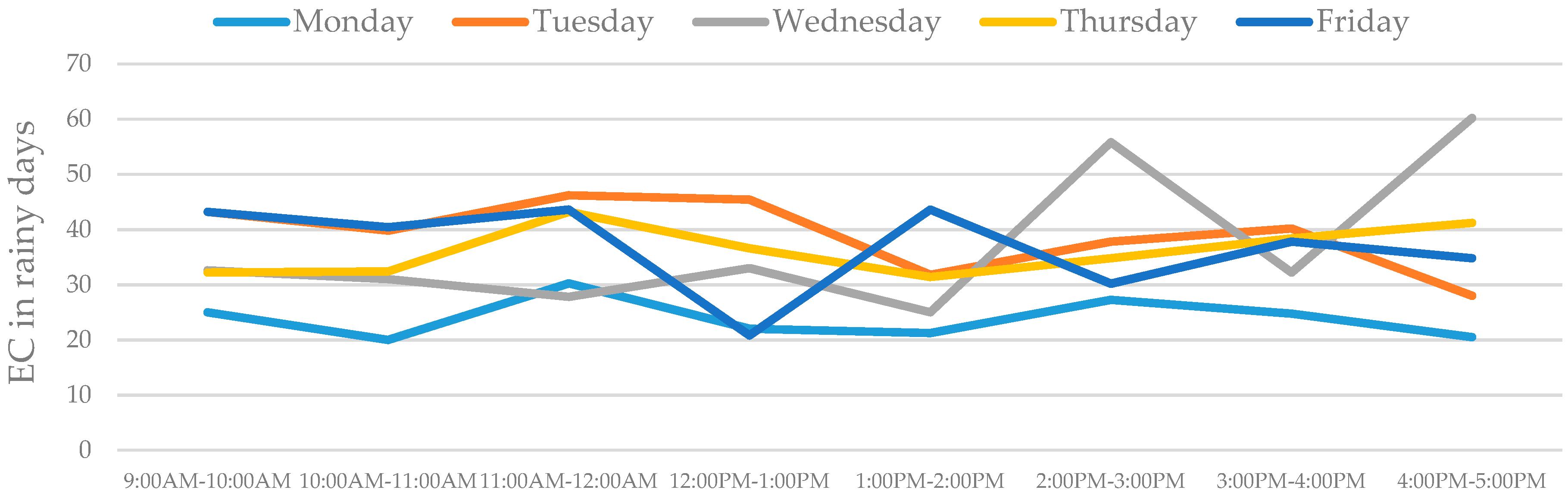
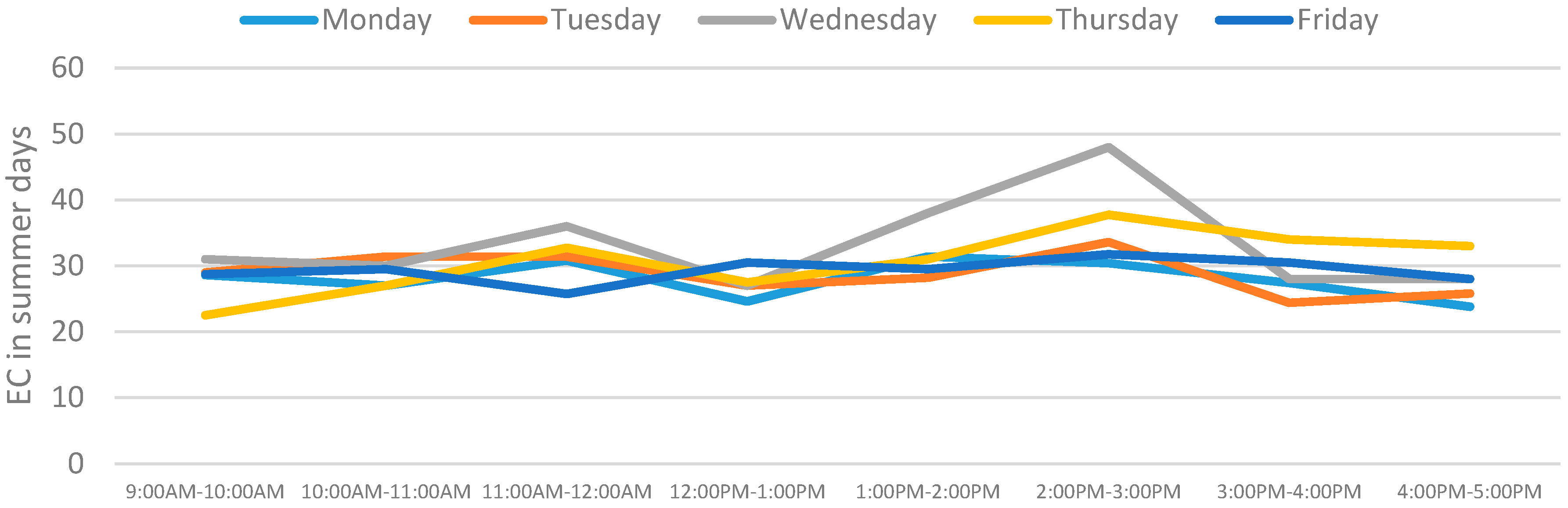
Figure 1, Figure 2 and Figure 3 represent the variation of average energy consumption for all Mondays, Tuesdays, Wednesdays, Thursdays, and Fridays in summer, rainy, and winter seasons, respectively. From the data, it can be observed that there is a significant variation in energy consumption from 9:00 a.m. to 5:00 p.m., and it is different on different days of the week.

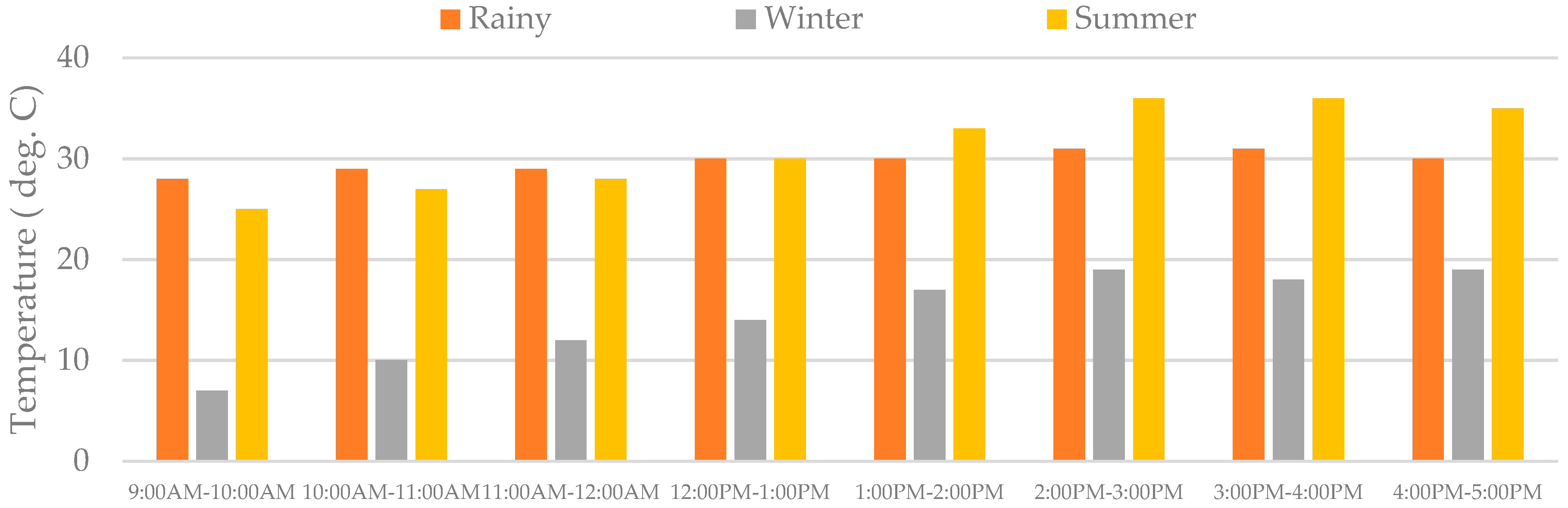
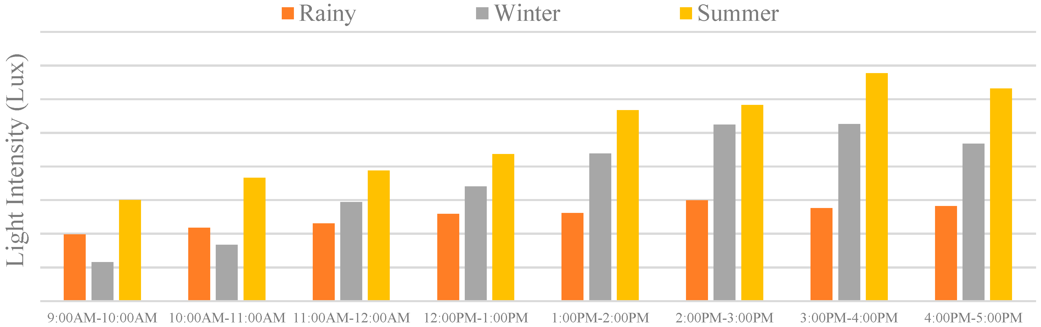
In addition to the above analysis, the monthly variation in energy consumption is shown in

Table 3. The average value of energy consumption (EC) in different seasons on an hourly basis.

Parameters and Time	Average EC in Rainy Season			Average EC in Winter Season			Average EC in Summer Season
	EC_FnT (kWh)	EC_AC (kWh)	EC_Total (kWh)	EC_FnT (kWh)	EC_AC (kWh)	EC_Total (kWh)	EC_FnT (kWh)	EC_AC (kWh)	EC_Total (kWh)
9:00–10:00 a.m.	40	7	47	10	0	10	10	4	14
10:00–11:00 a.m.	40	0	40	10	0	10	10	3	13
11:00 a.m.–12:00 p.m.	50	0	50	10	0	10	20	4	24
12:00–1:00 p.m.	30	0	30	0	0	0	20	4	24
1:00–2:00 p.m.	0	6	6	10	0	10	20	3	23
2:00–3:00 p.m.	10	4	14	10	0	10	10	5	15
3:00–4:00 p.m.	30	4	34	10	0	10	10	5	15
4:00–5:00 p.m.	0	4	4	0	0	0	10	5	15

. Also, temperature, humidity, and luminous intensity due to sunlight were evaluated in rainy, winter, and summer seasons, as shown in Figure 4, Figure 5 and Figure 6. Here also, these data were taken on an hourly basis, i.e., from 9:00 a.m. to 5:00 p.m. These data give the information of load variation of a complete day, which further helps in load shifting at the time of peak loads.

3.2. Energy Auditing of the Lighting System

In practice, all of the light emitted by the lamp does not reach the work area. Some light is absorbed by the luminaire, walls, floors, roof, etc. The illuminance measured in lumens/m², i.e., lux, indicates how much light, i.e., lumens, is available per square meter of the measurement plane. Target luminous efficacy (lm/watts) of the light source is the ratio of lumens that can be made available at the work plane under the best luminous efficacy of source, room reflectance, mounting height, and the power consumption of the lamp circuit. Over time, the light output from the lamp is reduced, the room surfaces become dull, and luminaries become dirty; hence, the light available on the work plane deviates from the target value. The ratio of the actual luminous efficacy on the work plane and the target luminous efficacy at the work plane is defined as the installed load efficacy ratio (ILER).

Table A1. Coefficient of utilization using the zonal cavity method [37].

RCC%	80				70				50			30			10			0
RW%	70	50	30	0	70	50	30	0	50	30	20	50	30	20	50	30	20	0
RCR:0	1.19	1.19	1.19	1.19	1.16	1.16	1.16	1.00	1.11	1.11	1.11	1.06	1.06	1.06	1.02	1.02	1.02	1.00
1	1.10	1.06	1.02	0.98	1.07	1.03	1.00	0.87	0.99	0.96	0.94	0.95	0.93	0.91	0.92	0.90	0.88	0.86
2	1.01	0.94	0.88	0.83	0.99	0.92	0.86	0.75	0.89	0.84	0.80	0.85	0.81	0.78	0.82	0.79	0.76	0.74
3	0.93	0.84	0.77	0.71	0.91	0.82	0.76	066	0.79	0.74	0.69	0.77	0.72	0.68	0.74	0.70	0.67	0.65
4	0.86	0.75	0.68	0.61	0.84	0.74	0.67	0.58	0.72	0.65	0.60	0.70	0.64	0.59	0.67	0.63	0.59	0.57
5	0.80	0.68	0.60	0.54	0.78	0.67	0.60	0.52	0.65	0.58	0.53	0.63	0.57	0.53	0.62	0.56	0.52	0.50
6	0.74	0.62	0.54	0.48	0.73	0.61	0.54	0.46	0.60	0.53	0.47	0.58	0.52	0.47	0.56	0.51	0.47	0.45
7	0.69	0.57	0.49	0.43	0.68	0.56	0.48	0.42	0.55	0.48	0.43	0.53	0.47	0.42	0.52	0.46	0.42	0.40
8	0.65	0.52	0.44	0.39	0.63	0.52	0.44	0.38	0.50	0.44	0.39	0.49	0.43	0.38	0.48	0.42	0.38	0.36
9	0.61	0.48	0.41	0.35	0.60	0.48	0.40	0.35	0.47	0.40	0.35	0.46	0.39	0.35	0.45	0.39	0.35	0.33
10	0.57	0.45	0.37	0.32	0.56	0.44	0.37	0.32	0.43	0.37	0.32	0.42	0.36	0.32	0.42	0.36	0.32	0.30

(Appendix A) shows the variation in the coefficient of utilization when effective floor cavity reflectance is taken as 20%.

Table 4. Energy efficiency evaluation of the lighting system of D-block in the rainy season.

Room No.	Eav	Lumens	ILE	ILER	Eav task	Eav, non-task	DF
D106	493.56	7355	15.01	0.33	422.50	510.10	0.83
D104	1231.42	130,485	100.37	2.18	1259.57	786.50	1.60
D107	814.10	12,133	93.33	2.03	643.83	537.50	1.20
D108	585.79	8730	67.16	1.46	558.17	383.50	1.46
D109	693.79	10,340	68.93	1.46	629.83	286.50	2.20
D110	693.79	10,340	68.93	1.46	629.83	286.50	2.20
D101	108.10	7332	8.15	0.18	102.55	68.86	1.49
D102	254.02	17,248	21.56	0.47	242.36	189.72	1.28
D116	621.43	120,326	46.28	1.07	781.36	448.25	1.74
D115	805.68	156,002	60.00	1.30	1059.57	613.32	1.73
Research Lab	236.95	7258	18.15	0.39	219.40	194.67	1.13
D201	1511.56	149,848	146.91	32.65	1361.07	247.25	5.50
D202	988.63	98,007	96.09	2.09	1361.29	825.50	1.65
D203	2478.17	125,252	379.55	8.25	2665.57	650.22	4.10
D204	1797.55	90,852	275.31	5.99	2399.93	1433.75	1.67
Cabin (S-Lab)	317.74	4675	23.38	0.51	294.20	261.13	1.13
Structure Lab	224.21	100,611	47.46	1.03	248.18	260.29	0.95
D120	108.43	1310	13.10	0.28	104.10	105.11	0.99
Cabin-1	1093.18	40,619	270.79	5.89	1142.83	2231.20	0.51
D112	611.71	51,450	64.31	1.39	707.36	585.20	1.21
Trans. Lab	291.82	38,871	64.79	1.41	253.36	263.57	0.96
D117	1036.37	35,897	358.97	7.80	959.60	1103.67	0.87
D114	358.99	5322	88.70	1.93	338.50	363.20	0.93
D113	358.99	5321	88.69	1.93	338.50	376.30	0.90
D111	440.86	15,238	126.99	2.76	616.07	604.67	1.02
D123	141.05	1704	17.04	0.37	125.00	142.50	0.88
Cabin-2	788.62	12,279	55.81	1.21	827.67	1766.50	0.47
D103	30.24	365	3.65	0.08	28.33	36.20	0.79
D118	252.07	16,155	16.48	0.36	216.14	236.25	0.91
Stair Room	181.87	2676	6.69	0.15	153.50	107.50	1.43
D119	273.89	3309	11.03	0.24	250.00	169.10	1.48
D121	309.74	4524	11.31	0.25	272.33	223.20	1.22
Corridor 1	620.57	281,189	562.38	12.23	566.43	448.25	1.26
Corridor 2	527.26	60,937	406.25	8.83	522.86	214.25	2.44

,

Table 5. Energy efficiency evaluation of the lighting system of D-block in the winter season.

Room No.	Eav	Lumens	ILE	ILER	Eav task	Eav, non-task	DF
D106	70.88	1056	2.16	0.05	57.50	90.10	0.64
D104	492.96	52,235	40.18	0.87	417.57	592.50	0.71
D107	80.19	1195	9.19	0.19	66.83	96.50	0.69
D108	67.51	1005	7.74	0.17	66.50	50.50	1.32
D109	215.73	3215	21.43	0.47	210.33	168.12	1.25
D110	215.73	3215	21.43	0.47	210.33	168.12	1.25
D101	118.20	8025	8.92	0.19	91.36	137.86	0.66
D102	132.72	9012	11.27	0.24	121.18	125.57	0.97
D116	749.22	145,069	55.79	1.21	688.14	713.25	0.96
D115	518.52	100,399	38.62	0.84	463.64	537.75	0.86
Research Lab	232.47	7121	17.80	0.39	239.40	175.11	1.37
D201	807.66	80,067	78.49	17.44	783.93	621.50	1.26
D202	910.14	90,226	88.46	1.92	790.07	1027.10	0.77
D203	257.70	13,024	39.47	0.86	241.29	229.25	1.05
D204	800.10	40,439	122.54	2.66	734.64	762.50	0.96
Cabin (S-lab)	365.18	5375	26.88	0.58	338.13	325.67	1.04
Structure Lab	958.98	430,335	202.99	4.41	1032.7	660.43	1.56
D120	105.17	1270	12.71	0.28	96.50	100.12	0.97
Cabin-1	96.26	3576	23.84	0.52	98	62.50	1.57
D112	270.06	22,714	28.39	0.62	228.27	284.29	0.80
Trans. Lab	737.52	98,241	163.74	3.56	587	833.57	0.70
D117	602.78	20,878	208.79	4.54	506.40	644.33	0.79
D114	83.70	1240	20.68	0.45	67.50	87.50	0.77
D113	81.95	1214	20.24	0.44	68.25	83.50	0.82
D111	220.86	7634	63.62	1.38	197.67	181.12	1.09
D123	116.10	1402	14.03	0.31	103.67	119.21	0.87
Cabin-2	71.82	1118	5.08	0.11	59.50	87.50	0.68
D103	166.73	2014	20.15	0.44	138	203.50	0.68
D118	177.84	11,397	11.63	0.25	158.29	187.22	0.85
Stair Room	1004.4	14,779	36.95	0.80	928.67	934.21	0.99
D119	162.81	1967	4.92	0.11	146.33	164.10	0.89
D121	131.35	1918	4.79	0.10	120.83	112.11	1.11
Corridor 1	527.31	238,933	477.87	10.39	355.57	314.75	1.13
Corridor 2	83.70	9673	64.49	1.40	72.50	74.25	0.98

and

Table 6. Energy efficiency evaluation of the lighting system of D-block in the summer season.

Room No.	Eav	Lumens	ILE	ILER	Eav, task	Eav, non-task	DF
D106	868.19	12,939	26.41	0.57	764.67	921.50	0.82
D104	1601.4	169,692	130.53	2.84	1273.21	1735.11	0.73
D107	1616.1	24,085	185.28	4.02	1562.33	1724.50	0.91
D108	224.42	3344	25.73	0.56	216.67	326.12	0.66
D109	475.85	7091	47.28	1.03	508.33	654.50	0.78
D110	475.85	7091	47.28	1.03	508.33	654.50	0.78
D101	1139.18	77,343	85.94	1.87	1245.73	1630.57	0.76
D102	618.84	42,021	52.53	1.14	653.64	555.86	1.18
D116	2723.33	527,311	202.81	4.41	2314.64	2639.21	0.88
D115	1840.32	356,337	137.05	2.98	2110.07	2286.20	0.92
Research Lab	1055.10	32,322	80.81	1.76	977	928.67	1.05
D201	1469.66	145,694	142.84	31.74	964.64	1100.10	0.88
D202	1383.69	137,172	134.48	2.92	847	654.75	1.29
D203	1017.36	51,419	155.82	3.38	885.21	610.75	1.45
D204	1127.52	56,987	172.69	3.75	1530.64	1261.25	1.21
Cabin (S-lab)	317.74	376	1.88	0.04	281.88	61.11	4.61
Structure Lab	1419.55	637,013	300.47	6.53	1350.09	1412.14	0.96
D120	830.30	10,033	100.33	2.18	739.67	676.50	1.09
Cabin-1	400.25	14,872	99.15	2.16	349.67	383.12	0.91
D112	1251.72	105,280	131.60	2.86	1074.64	1091.14	0.98
Trans. Lab	6978.7	929,609	1549.30	33.68	3600	5730.29	0.63
D117	1378.5	47,748	477.48	10.38	1276.4	659.67	1.93
D114	510.41	7567	126.12	2.74	416.25	518.25	0.80
D113	472.82	7008	116.81	2.54	371	537.25	0.69
D111	1234.8	42,683	355.69	7.73	1209.27	1208.10	1.00
D123	207.14	2503	25.03	0.54	203	153.50	1.32
Cabin-2	304.34	4738	21.54	0.47	293.33	353.50	0.83
D103	308.88	3732	37.32	0.81	263.33	172.50	1.53
D118	1187.3	76,096	77.65	1.69	1047.57	811.25	1.29
Stair Room	1235.5	18,180	45.45	0.99	1034	772.50	1.34
D119	989.71	11,959	29.89	0.65	889.33	944.50	0.94
D121	1070.49	15,638	39.09	0.85	970	809.50	1.19
Corridor 1	1423.66	645,082	1290.17	28.05	1199.71	86.25	1.40
Corridor 2	893.60	103,277	688.52	14.97	1304.64	382.50	3.41

show the readings of monthly data, which include the average light intensity and its value in task and non-task areas, lumens, ILE and ILER, and the diversity factor for each room of the sample building in rainy, winter, and summer seasons respectively.

From the results shown in Table 4, Table 5 and Table 6, it can be observed that the value of average illuminance is different in different seasons for the same room. It further tends to vary the ILE, ILER, and DF. A lower value of ILER indicates that the luminous efficacy of the installed luminaires is poor, whereas a low value of DF is the indication of uniform distribution of light intensity in the specified area irrespective of the task and non-task areas.

Table 7. Room index and cavity ratio, IMP, and the number of light sources.

Room No.	RI	RCR	IMPtask	IMPnon-task	NL
D106	0.70	0.47	5.6	2.4	5
D104	1.89	0.18	14.4	3.6	32
D107	0.70	0.47	5.6	2.4	5
D108	0.70	0.47	5.6	2.4	5
D109	0.70	0.47	5.6	2.4	5
D110	0.70	0.47	5.6	2.4	5
D101	1.48	0.23	10.8	7.2	20
D102	1.48	0.19	10.8	7.2	20
D116	1.92	0.19	13.5	4.5	58
D115	1.92	0.41	13.5	4.5	58
Research Lab	0.82	0.20	4.8	3.2	9
D201	1.73	0.20	13.5	4.5	30
D202	1.73	0.28	13.5	4.5	30
D203	1.20	0.28	13.5	4.5	15
D204	1.20	0.73	13.5	4.5	15
Cabin (S-lab)	0.51	0.73	4.8	3.2	5
Structure Lab	1.59	0.25	10.8	7.2	136
D120	0.41	0.93	5.6	2.4	4
Cabin-1	0.66	0.58	5.6	2.4	12
D112	1.68	0.20	10.8	7.2	25
Trans. Lab	1.41	0.26	10.8	7.2	40
D117	0.61	0.63	5.2	2.8	11
D114	0.41	0.94	4	4	5
D113	0.41	0.94	4	4	5
D111	1.05	0.32	15.3	2.7	11
D123	0.41	0.93	5.6	2.4	4
Cabin-2	0.71	0.46	5.6	2.4	5
D103	0.41	0.93	5.6	2.4	4
D118	1.39	0.24	14.4	3.6	19
Stair Room	0.51	0.73	5.6	2.4	5
D119	0.41	0.93	5.6	2.4	4
D121	0.67	0.51	5.6	2.4	5
Corridor 1	1.28	0.26	13.5	4.5	10
Corridor 2	1.20	0.31	13.5	4.5	3

shows the various parameters of room index (RI) and room cavity ratio (RCR), as well as IMPs for task and non-task areas, which were obtained based upon the size of the room. Based upon the data available in Table 4, Table 5 and Table 6 the number of luminaires (N_L) was calculated with a poor value of average light intensity so that the minimum illuminance could be maintained even under the worst conditions.

3.3. Energy Auditing of Ventilation System

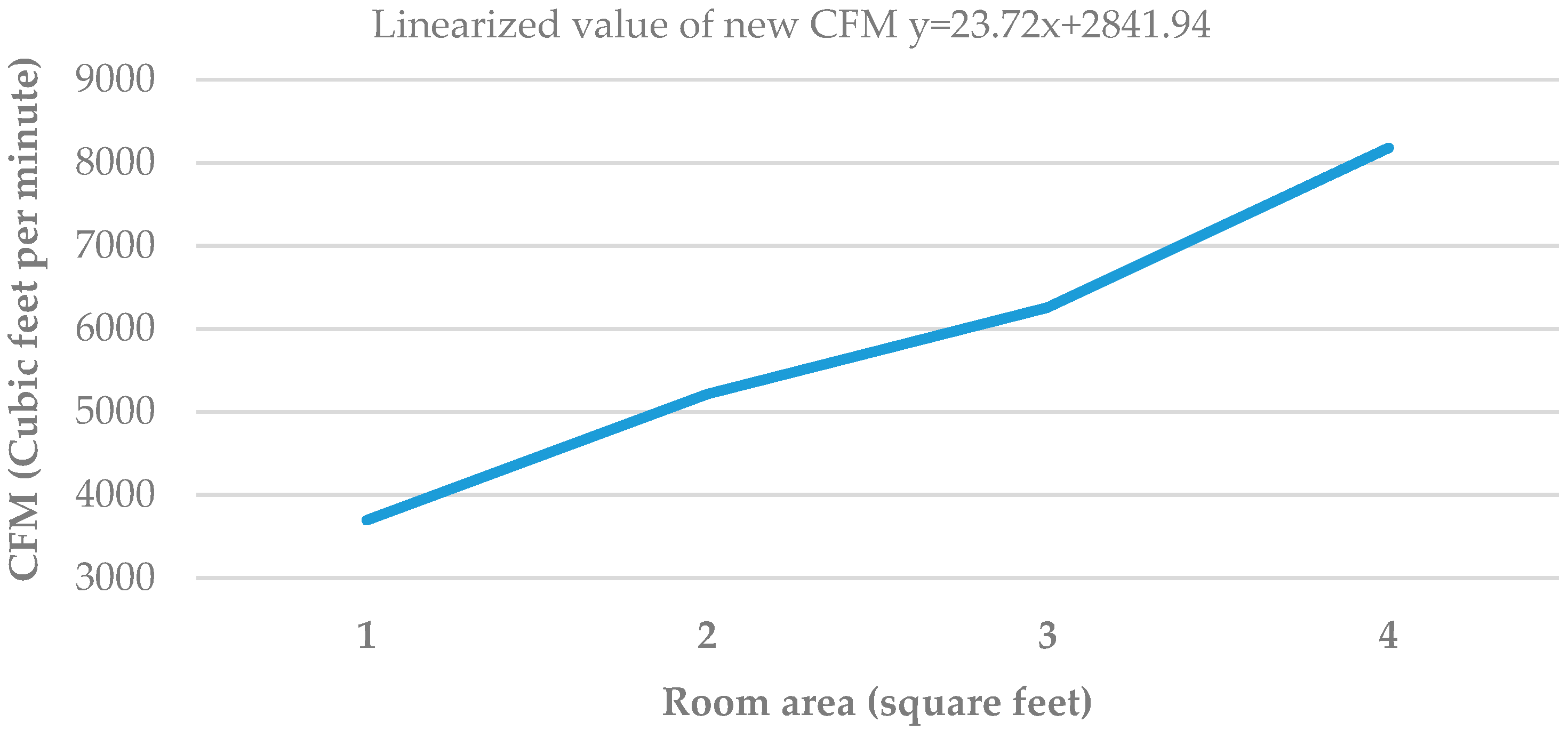
Linearization of CFM for Fan Requirement

Table 8. Mathematical calculations for the analysis of fans.

S. No.	Room Area (x)	CFM Recommended	Average CFM (y)	x × y	(x2)	$\mathbf{Linearized} \mathbf{Value} \mathbf{of} \mathbf{New} \mathbf{CFM} \widehat{\mathit{y}} = 23.72\mathit{x} + 2841.94$
1	36	3000–4500	3750	135,000	1296	3695.86
2	100	4000–5500	4750	475,000	10,000	5213.94
3	144	6200–7500	6850	986,400	20,736	6257.62
4	225	7000–9000	8000	1,800,000	50,625	8178.94
Sum	505	-	23,350	3,396,400	82,657	-

shows the recommended level of cubic feet per minute (CFM) of air circulation in a specified area. These data were available for the limited size of the rooms, whereas, in the analysis, the room size was a little big and, therefore, a linear aggression function was derived using Equations (20)–(22). These data give information about the number of fans that should be installed as per the recommendation in a specified area. The linearized function is derived as

$$\widehat{y}=mx+b$$

(20)

where m represents the slope of the line, and b represents the y-intercept (y-value for which x is 0).

$$m=\frac{n{{\displaystyle \sum }}^{}xy-\left({{\displaystyle \sum }}^{}x\right)\left(y\right)}{n{{\displaystyle \sum }}^{}(x^2)-n{({{\displaystyle \sum }}^{}x)}^2}.$$

(21)

$$b=\frac{{{\displaystyle \sum }}^{}y}{n}-m\frac{{{\displaystyle \sum }}^{}x}{n}.$$

(22)

In Equation (20), $\widehat{y}$ is the predicted value of y. The linear regression line is the representation of Equation (20) in which m and b are obtained using Equations (21) and (22), and, from the calculation, their values were found to be 23.72 and 2841.94, respectively. Figure 7 shows the graph between the area of a room (in square feet) and the CFM (cubic feet/min).

Table 9. Detailed information and data analysis of fans.

Room No.	Area		Volume		Fan Size (37 to 48 inches)
	ft2	m2	ft3	M3	CFM	Fan
D106	160.34	14.89	1349.51	38.23	6645.19	1.58
D104	1140	105.91	10,069.62	285.21	29,882.74	7.11
D107	160.34	14.89	1349.51	38.23	6645.19	1.58
D108	160.34	14.89	1349.51	38.23	6645.19	1.58
D109	160.34	14.89	1349.57	38.23	6645.19	1.58
D110	160.34	14.89	1349.57	38.23	6645.19	1.58
D101	730.43	67.86	6634.49	187.91	20,167.72	4.80
D102	730.53	67.87	6635.37	187.94	20,170.03	4.80
D116	2083.13	193.53	24,649.62	698.17	52,253.67	12.44
D115	2083.13	193.53	24,649.62	698.17	52,253.67	12.44
Research Lab	329.56	30.62	2966.04	84.01	10,659.10	2.54
D201	1066.53	99.08	10,043.51	284.47	28,140.03	6.70
D202	1066.53	99.08	10,043.51	284.47	28,140.03	6.70
D203	543.76	50.52	5120.56	145.03	15,739.85	3.75
D204	543.76	50.52	5120.56	145.03	15,739.85	3.75
Cabin (S-lab)	158.31	14.71	1965.76	55.68	6597.09	2
Structure Lab	4827.75	448.51	77,646.15	2199.24	117,356.20	27.94
D120	130	12.077	1798.29	50.93	5925.54	1.41
Cabin-1	399.75	37.14	5529.74	156.62	12,324.01	2.93
D112	904.88	84.06	8068.41	228.53	24,305.58	5.79
Trans. Lab	1433.08	133.14	18,510.54	524.29	36,834.63	8.77
D117	372.65	34.62	5310.19	150.41	11,681.08	2.78
D114	159.49	14.82	2299.48	65.13	6625.23	1.58
D113	159.47	14.82	2299.11	65.12	6624.62	1.58
D111	371.87	34.55	3408.77	96.55	11,662.67	2.78
D123	130	12.08	1798.29	50.93	5925.54	1.41
Cabin-2	167.51	15.56	1409.96	39.94	6815.37	1.62
D103	130	12.08	1797.90	50.92	5925.54	0.68
D118	689.49	64.06	6435.10	182.27	19,196.87	4.57
Stair Room	158.31	14.71	1965.76	55.68	6597.09	1.57
D119	130	12.08	1798.29	50.93	5925.54	1.41
D121	157.17	14.60	1480.05	41.92	6569.95	1.56

shows the room area and volume for the calculation of CFM required in a specified area, which further helps in the calculation of the number of fans. Here, it can be observed that the number of fans which should be installed in each room was different, which was obtained using linear regression. As a result, two rooms having the same area would also have the same number of fans according to this criterion.

3.4. Energy Auditing of the Air Conditioning System

Table 10. Detailed information about the AC system.

Room No.	Recommended BTU/kW in the Different Room [27]		AC Size in Tons Using Different Methods Based on
			Area			Volume
	BTU Recommended	kW	BTU [28]	Criterion 1 [29]	Criterion 2 [29]	Criterion 3 [29]
D106	6000	1.76	4008.49	0.33	1.27	1.35
D104	17,700	5.19	28,500.00	2.38	3.38	10.07
D101	15,000	4.40	18,260.73	1.52	2.70	6.63
D102	15,000	4.40	18,263.17	1.52	2.70	6.64
Research Lab	7250	2.12	8239.00	0.69	1.82	2.97
D201	17,700	5.19	26,663.24	2.22	3.26	10.04
D202	17,700	5.19	26,663.24	2.22	3.27	10.04
D203	10,500	3.08	13,593.92	1.13	2.33	5.12
D204	10,500	3.08	13,593.92	1.13	2.33	5.12
Cabin (S-lab)	6000	1.76	3957.79	0.33	1.26	1.97
D112	15,000	4.40	22,621.88	1.89	3.01	8.07
Cabin-2	6000	1.76	4187.84	0.35	1.29	1.41
D118	12,500	3.66	17,237.49	1.44	2.63	6.44
D119	5000	1.47	3250.00	0.27	1.14	1.79

shows the auditing details of the AC installation. Here, the rooms equipped with ACs were taken into consideration, whereas the other rooms in which ACs are not installed, were ignored.

For AC recommendations, four different criteria were studied as shown in Table 10. From the analysis, it can be observed that the number or size of ACs was different in each specified area. In the second column of Table 10, the BTU recommendation is shown, which was decided based upon the room size. The equivalent representation of the BTU was also converted into kW of its rating for comparison with other criteria. 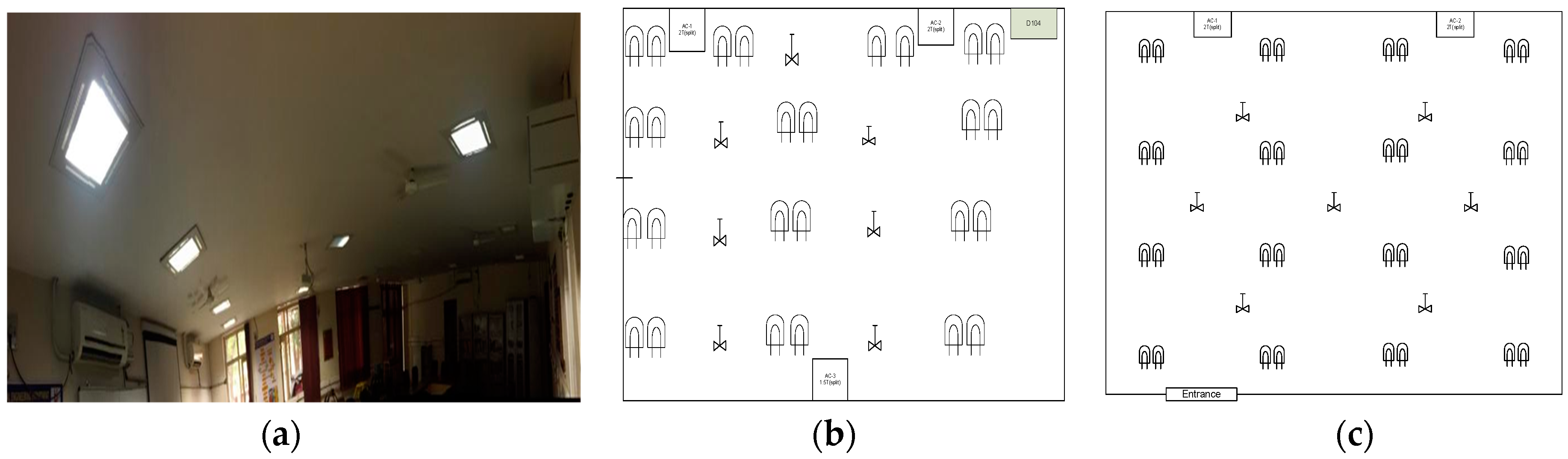Figure 8 shows the physical layout of the power components in a sample room in the commercial building. Before auditing, the power components were placed at random, whereas, after auditing, they were placed uniformly such that the ILER, DF, CFM, and BTU requirements could be maximized in the task area.

4. Energy Efficiency with DSM

DSM is a cost-effective means to reduce peak load demand by reshaping the load profile [10]. However, in commercial and residential buildings, load shifting is rare; rather, it needs to be managed according to the requirement. This allows operating the number of power components based on the framework designed for their operating schedule. The operating schedule of various components may vary with application and their recommendation for specific purposes. In this scenario, operating schedules applicable under some circumstances, at the same time, may be different from other systems of the same size. Therefore, the implementation of DSM schemes should have the flexibility to meet the objective of power-saving and, hence, to improve energy efficiency without affecting the comfort level [12].

The objective function for DSM was formulated for energy-saving to minimize the cost of the customer electricity bill. Therefore, the DSM problem for energy-saving is described in Equation (23).

$$\{\begin{array}{c}Minimize f_x\\ f_x ={\displaystyle {\displaystyle \sum }_{r=1}^{NR}}{\displaystyle {\displaystyle \sum }_{t=1}^8}{P}_{rt}\times T_{rt}\times E{P}_{rt}\end{array}$$

(23)

In the proposed work, the load demand (P_rt) was calculated for each room; therefore, r varied from one to NR, i.e., the number of rooms in a sample building, and energy efficiency was evaluated for $T_{rt}$, i.e., the duration in a day where t varies from 1–8. Conversely, $E{P}_{rt}$ is the energy price at the time t, which in this case was the same for all loads; however, in practice, it may be different in the case of DR-based DSM approaches. The objective function was subject to the following constraints:

• Energy consumption: The new energy consumption (EC) should be less than the existing consumption, which is represented in Equation (24).

  $${{\displaystyle \sum }}^{}E{C}_{new, rt}\le {{\displaystyle \sum }}^{}E{C}_{old, rt.}$$

  (24)
• Illuminance level: The light intensity of the light source is different, and it is also affected by the power rating. Therefore, the illuminance level should be maintained between the minimum and the maximum level, which is represented in Equation (25).

  E_avg,min < E_avg < E_avg,max.

  (25)
• Persons involved: The number of persons (N_p) involved in a specified area varies throughout the day. Therefore, the minimum and maximum numbers need to be defined before the DSM implementation, which is represented in Equation (26).

  N_{p, min} < N_p < N_{p, max}.

  (26)
• Temperature and humidity: The number of fans and ACs to be operated can be affected by the surrounding temperature (ST) and the humidity (H). However, the humidity level in both winter and rainy seasons is usually high; however, the operation of fans and ACs can only be affected on rainy days due to high temperatures. Therefore, before imposing the constraint of humidity, the surrounding temperature needs to be considered, which is represented in Equations (27) and (28).

  ST_min < ST < ST_max.

  (27)

  H_min < H < H_max.

  (28)

Equations (24) and (25) represent the technical constraints where energy consumption affects the objective function, whereas Equation (26) represents the social constraint, which mainly depends upon the human being involved in a specified area. However, Equations (27) and (28) represent the environmental constraints, as temperature varies from severe cold to severe heat with different levels of humidity.

4.1. Operating Scenario for DSM

In commercial and residential buildings, power consumption mainly depends upon the number of persons involved, surrounding temperature and humidity, and the luminous intensity due to sunlight [23]. Therefore, the energy data of three months in a year were collected under three different seasonal changes, i.e., January (severe cold), April (moderate), and August (severe heat), as described in Section 3. This was done to show the significant variation in load demand under moderate, comfortable, and severe environmental conditions. The energy data under these three conditions were averaged, and the operating scenario for DSM schemes was developed, as shown in

Table 11. The operating scenario for demand-side management (DSM).

Components/Schedule	1	2	3	4	5	6	7	8	9	10	11	12	13	14
Strength	0	5	10	20	30	40	50	60	70	80	90	100	110	120
Light	0	4	8	12	16	20	24	28	32	36	40	44	48	52
Fan	0	2	3	4	5	6	8	10	11	12	13	14	15	16
AC	0	1	1	1	1	1	2	2	2	3	3	3	4	4

, for the operation of power components before energy auditing and after energy auditing.

The operating scenario, described in Table 11, represents the initial solution for the maximum number of lights, fans, and ACs that can be operated for the predefined strength, i.e., number of persons in a specified area. However, during operation, the above scenario can be adjusted with a minimum step size of $\pm$1 to limit the violation of the constraints.

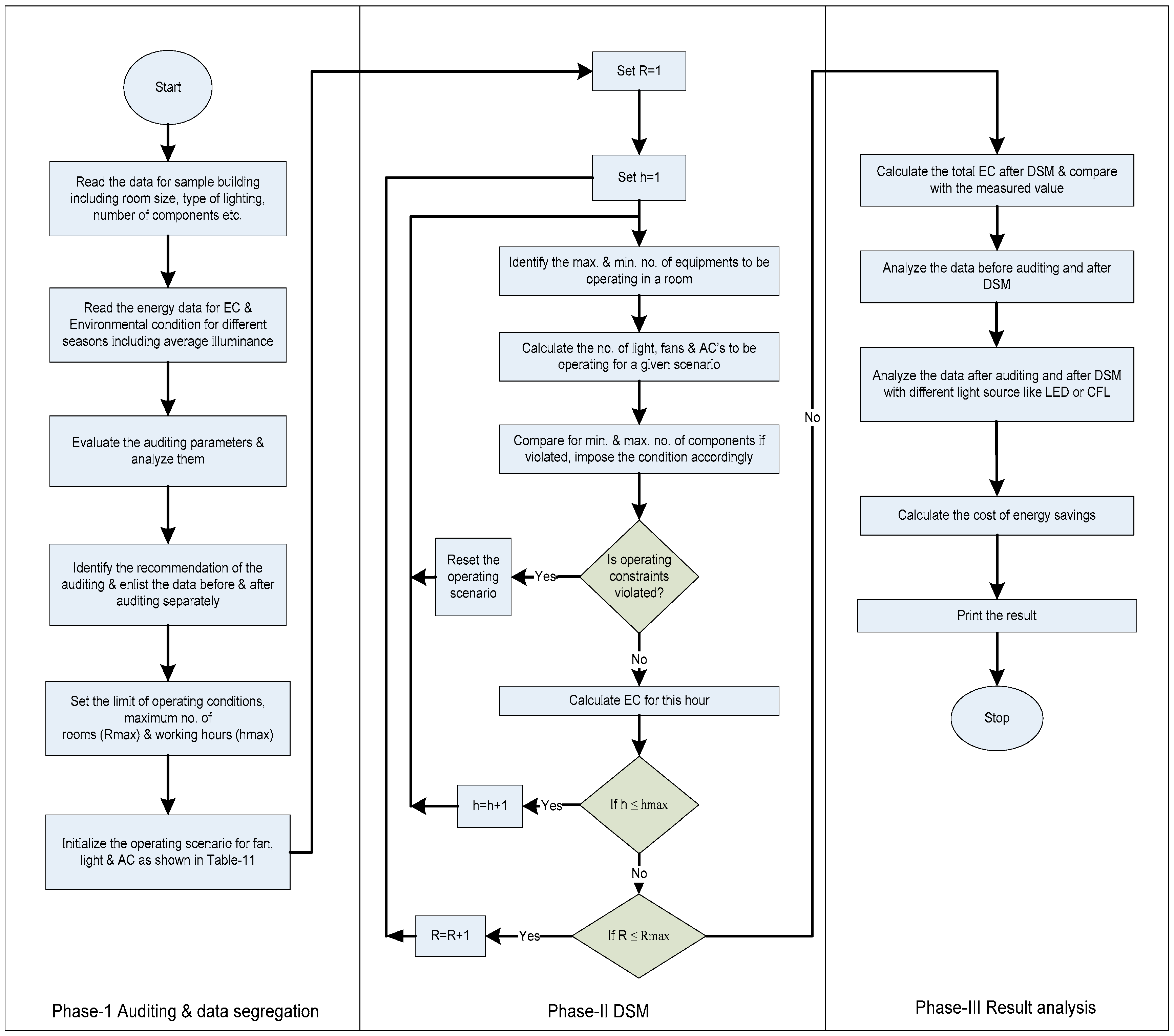
4.2. Proposed DSM-Based Algorithm and its Flowchart

In Section 3, strategic auditing was presented for different seasons, and the results in Table 4, Table 5, Table 6, Table 7, Table 8, Table 9 and Table 10 show that there is significant variation in different auditing parameters. Therefore, auditing before DSM does not only tell us about the immediate scope of energy-saving; rather, it helps to develop a framework of the operating scenario and constraints in the DSM approach. Based upon the findings from strategic auditing and the operating scenario for DSM, an algorithm was developed, and Figure 9 shows the flowchart of the proposed DSM approach.

The steps involved in the proposed DSM-based algorithm are described below.

• Read the actual data before auditing the sample building, including the size of the rooms, number of persons involved in each room, number of power components and their specifications, types of rooms, and the time of operation.
• Read the measurement data for energy consumption and the surrounding environment in different seasons for the analysis.
• Calculate the various auditing parameters using Equations (1)–(19).
• Identify the recommendations of strategic auditing and enlist the number of power components in each room with their power ratings.
• Enlist the above data before auditing and after auditing separately.
• Set the limits for operating constraints, the maximum number of rooms (R_max), and working hours (h_max).
• Initialize the operating scenario for fans, lights, and ACs, as shown in Table 11.
• Initialize the number of rooms and set R = 1.
• Initialize the working hours and set h = 1.
• Define the maximum and the minimum number of components to be operated in a specific room.
• Calculate the number of lights, fans, and ACs to be operating for a given scenario.
• Compare the components in steps 10 and 11; then, impose the conditions as per step 10 for maximum and minimum limits accordingly.
• Check operating constraints; if violated, adjust the operating scenario and repeat steps 9–12; otherwise, go to the next step.
• Calculate the energy consumption due to fans, lights, and ACs, as well as the energy-saving for this hour.
• Check for h ≤ h_max; if yes, set h = h + 1 and repeat steps 10–14; otherwise, go to the next step.
• Check for R ≤ R_max; if yes, set R = R + 1 and repeat steps 9–15; otherwise, go to the next step.
• Calculate cumulative energy-saving in a day and a year using Equation (23) and compare with the measured value.
• Calculate the cost of saving.
• Stop.

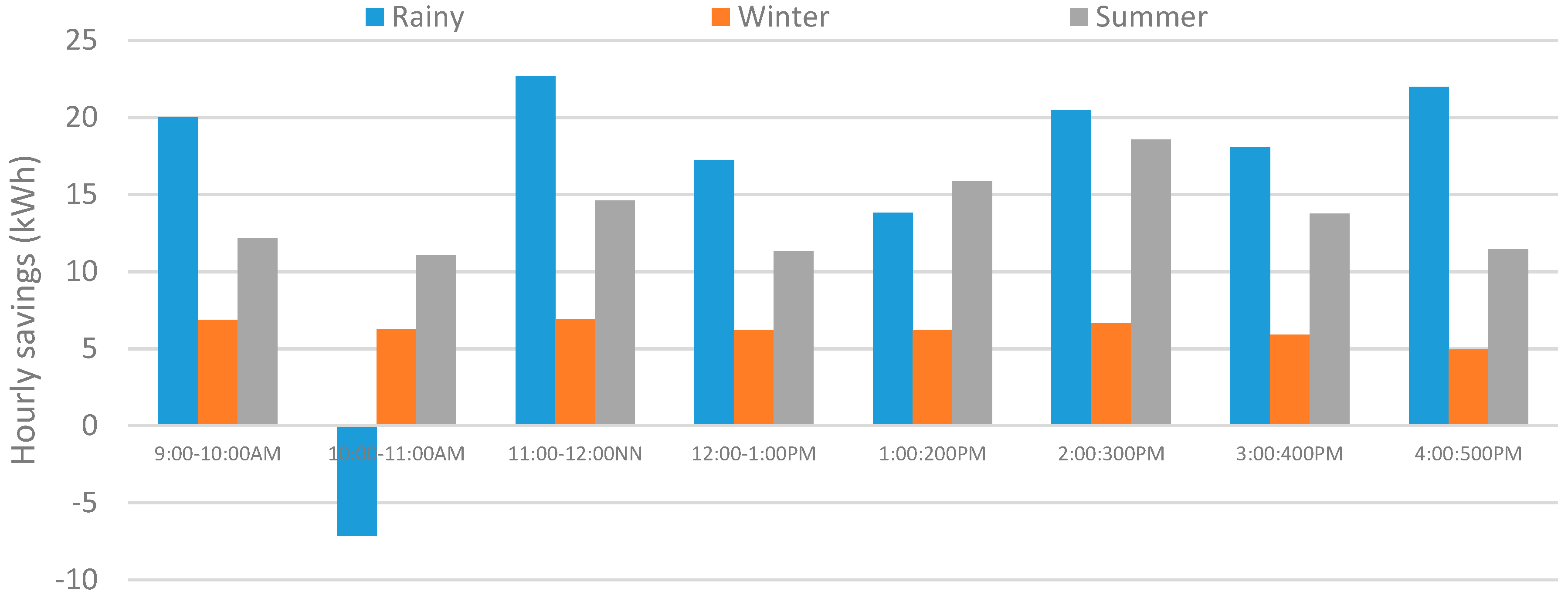
5. Result Analysis for DSM Before Auditing

The energy efficiency was evaluated before and after auditing.

Table 12. DSM before auditing in the rainy season.

Parameter/Time (a.m./p.m.)	9:00–10:00 a.m.	10:00–11:00 a.m.	11:00 a.m.–12:00 p.m.	12:00–1:00 p.m.	1:00–2:00 p.m.	2:00–3:00 p.m.	3:00–4:00 p.m.	4:00–5:00 p.m.
SR	0.4	0.4	0.5	0.4	0.3	0.6	0.3	0.3
Temp (°C)	27.95	29.00	29.75	30.875	30.875	31.17	30.83	29.88
Humidity (%)	79.29	80.67	77.83	71.25	72.08	70.54	72.04	75.38
LI (Lux)	18,378	21,245	22,926	26,550	25,945	26,424	24,033	21,999
ECLT (kWh)	11.85	11.90	12.65	11.55	11.55	11.75	11.75	11.15
ECAT (kWh)	11.40	36.48	11.40	6.84	13.68	13.68	13.68	11.40
ECFT (kWh)	3.84	3.96	3.96	4.92	5.34	5.46	5.28	3.90
ECTT (kWh)	27.09	52.34	28.01	23.31	30.57	30.89	30.71	26.45
ECWDSM (kWh)	35.67	33.25	38.54	31.96	31.00	37.58	35.08	37.63
Savings (kWh)	8.58	−19.09	10.53	8.65	0.43	6.69	4.37	11.18

,

Table 13. DSM before auditing in the winter season.

Parameter/Time (a.m./p.m.)	9:00–10:00 a.m.	10:00–11:00 a.m.	11:00 a.m.–12:00 p.m.	12:00–1:00 p.m.	1:00–2:00 p.m.	2:00–3:00 p.m.	3:00–4:00 p.m.	4:00–5:00 p.m.
SR	0.4	0.3	0.2	0.1	0.0	0.2	0.3	0.0
Temp (°C)	9.58	11.50	13.75	15.25	17.21	18.42	18.42	18.46
Humidity (%)	85.21	77.54	71.25	66.88	61.08	58.04	57.54	58.38
LI (Lux)	1160	16,717	29,437	34,026	43,801	52,450	52,602	46,745
ECLT (kWh)	15.93	15.80	14.90	12.55	12.50	11.95	11.15	11.55
ECAT (kWh)	0	0	0	0	0	0	0	0
ECFT (kWh)	0	0	0	0	0	0	0	0
ECTT (kWh)	15.93	15.80	14.90	12.55	12.50	11.95	11.15	11.55
ECWDSM (kWh)	10.83	10.42	10.83	9.58	9.58	9.17	8.75	7.92
Savings (kWh)	−5.09	−5.38	−4.07	−2.97	−2.92	−2.78	−2.40	−3.63

and

Table 14. DSM before auditing in the summer season.

Parameter/Time (a.m./p.m.)	9:00–10:00 a.m.	10:00–11:00 a.m.	11:00 a.m.–12:00 p.m.	12:00–1:00 p.m.	1:00–2:00 p.m.	2:00–3:00 p.m.	3:00–4:00 p.m.	4:00–5:00 p.m.
SR	0.2	0.3	0.4	0.1	0.1	0.2	0.3	0.0
Temp (°C)	29.78	31.96	33.35	34.65	36.26	37.39	37.78	37.22
Humidity (%)	47.04	43.00	37.30	33.13	28.39	26.91	25.22	24.96
LI (Lux)	31,926	36,961	43,475	5477	67,048	73,032	74,209	70,848
ECLT (kWh)	12.20	12.60	12.50	11.75	0	0	0	0
ECAT (kWh)	13.68	13.68	11.40	13.68	13.68	11.40	13.68	11.40
ECFT (kWh)	3.84	5.34	5.10	5.46	5.28	5.28	5.28	5.34
ECTT (kWh)	29.72	31.62	29.00	30.89	18.96	16.68	18.96	16.74
ECWDSM (kWh)	27.91	28.32	29.32	28.32	29.77	32.55	27.55	25.50
Savings (kWh)	−1.81	−3.30	0.32	−2.57	10.81	15.87	8.59	8.76

show the results for the DSM scheme before auditing for three different seasons in a year. The various parameters like strength ratio (SR), temperature in °C, relative humidity, luminous intensity (LI), energy consumption of light (ECLT), energy consumption of ACs (ECAT), energy consumption of fans (ECFT), total energy consumption (ECTT) which is the sum of ECLT, ECAT and ECFT, energy consumption with DSM (ECWDSM) and the savings as the difference of ECTT and ECWDSM.

The cumulative energy-saving, shown in the last row of Table 12, Table 13 and Table 14, in rainy and summer seasons was found to be 31.34 and 36.67 kWh, respectively, whereas, in the winter, it was −29.24 kWh. This issue indicates that, with DSM, the energy consumption reduced in rainy and summer seasons, whereas it increased in the winter season. This is because, in the winter season, the weather conditions are very cold, and the maximum light source requires operation to maintain the recommended level of illuminance. Also, at the same time there is no scope of energy-saving due to fans and ACs because they remain OFF in the winter season.

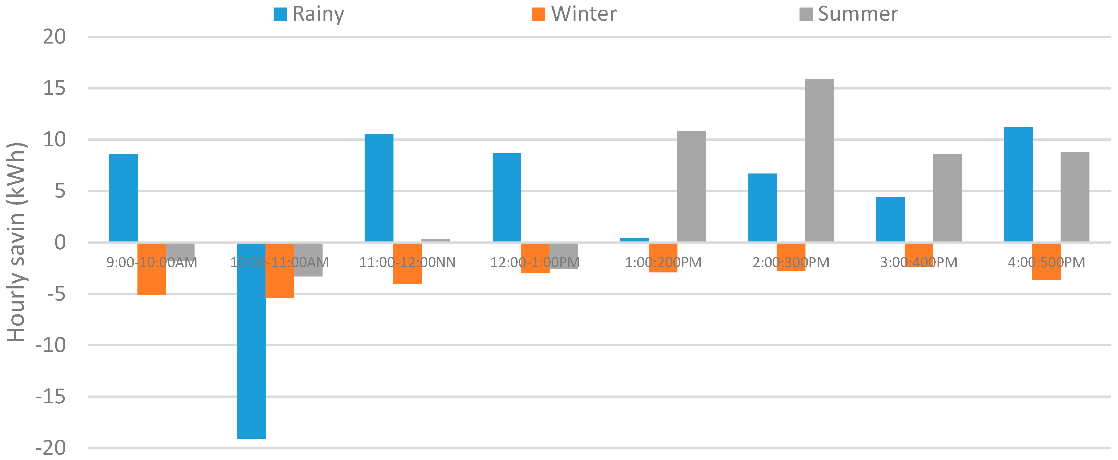
Figure 10 represents the variation of hourly energy-saving in different seasons, as shown in the last row of Table 12, Table 13 and Table 14. Here, it can be noted that the energy consumption reduced from 9:00 a.m. to 10:00 a.m. in the rainy season, whereas it increased in the summer and winter seasons, even after DSM. Furthermore, the energy-saving (in blue color) in different hours in the rainy season was found to be different. Also, from 10:00 a.m. to 11:00 a.m., the energy-saving was found to be negative, which means that consumption is higher even after DSM for this duration. Similarly, in summer, the energy-saving, shown in gray color, varied differently throughout the day and, the energy-saving (in orange color) in winter was negative concerning the consumption before DSM. However, the cumulative saving in three different seasons was found to be positive for the proposed DSM approach.

6. Results and Discussion for DSM after Auditing

In this section, the results of DSM after auditing are discussed. In the proposed work, after auditing, the DSM was implemented in two ways: (a) when light sources were LEDs having a power rating of 13 W, and (b) when light sources were CFLs having a power rating of 22 W.

6.1. DSM after Auditing When the Light Source Is LED

Table 15. Results of DSM for energy efficiency after auditing with LED.

Part-A DSM with Auditing in the Rainy Season
Parameter/Time (a.m./p.m.)	9:00–10:00 a.m.	10:00–11:00 a.m.	11:00 a.m.–12:00 p.m.	12:00–1:00 p.m.	1:00–2:00 p.m.	2:00–3:00 p.m.	3:00–4:00 p.m.	4:00–5:00 p.m.
ECLT (kWh)	3.12	2.82	3.23	3.06	3.09	3.00	3.03	2.97
ECAT (kWh)	9.12	34.20	9.12	6.84	9.12	9.12	9.12	9.12
ECFT (kWh)	3.42	3.36	3.54	4.86	4.98	4.98	4.86	3.54
ECTT (kWh)	15.66	40.38	15.89	14.76	17.19	17.10	17.01	15.63
ECWDSM (kWh)	35.67	33.25	38.54	31.96	31	37.58	35.08	37.63
Savings (kWh)	20.00	-7.13	22.65	17.20	13.81	20.48	18.08	21.99
Part-B DSM with Auditing in the Winter Season
ECLT (kWh)	3.96	4.16	3.92	3.38	3.36	3.00	2.84	2.96
ECAT (kWh)	0	0	0	0	0	0	0	0
ECFT (kWh)	0	0	0	0	0	0	0	0
ECTT (kWh)	3.96	4.16	3.92	3.38	3.36	3.00	2.84	2.96
ECWDSM (kWh)	10.83	10.42	10.83	9.58	9.58	9.17	8.75	7.92
Savings (kWh)	6.87	6.26	6.92	6.21	6.23	6.66	5.91	4.96
Part-C DSM with Auditing in Summer Season
ECLT (kWh)	3.14	3.31	3.14	3.06	0	0	0	0
ECAT (kWh)	9.12	9.12	6.84	9.12	9.12	9.12	9.12	9.12
ECFT (kWh)	3.48	4.80	4.74	4.80	4.80	4.86	4.68	4.92
ECTT (kWh)	15.74	17.23	14.72	16.98	13.92	13.98	13.80	14.04
ECWDSM (kWh)	27.91	28.32	29.32	28.32	29.77	32.55	27.55	25.50
Savings (kWh)	12.17	11.09	14.60	11.34	15.85	18.57	13.75	11.46

shows the result of DSM after auditing in rainy, winter, and summer seasons when the light source is LED. The cumulative energy-saving in rainy and summer seasons was found to be 127.09 and 108.83 kWh, respectively, whereas, in the winter season, it was 49.52 kWh. This indicates that, with DSM, the energy consumption reduced significantly in the rainy and summer seasons, whereas, unlike DSM before auditing, the energy consumption also reduced in the winter season.

Figure 11 represents the variation in energy-saving, shown under “savings” of each part of Table 15, for the different seasons in a year. From the results, unlike savings in Table 12, Table 13 and Table 14, it can be observed that the reduction in energy consumption in winter was positive throughout the day except at 10:00–11:00 a.m.; however, it was less compared to rainy and summer seasons, because in winter the weather conditions are very cold, and the maximum light source needs to be operated to maintain the desired level of illuminance. As a result, more light sources are operated, and energy-saving at 10:00–11:00 a.m. becomes negative, as shown in Figure 11.

6.2. DSM after Auditing When the Light Source Is CFL

Table 16. Results of DSM for energy efficiency after auditing with CFL.

Part-A DSM with Auditing in the Rainy Season
Parameter/Time (a.m./p.m.)	9:00–10:00 a.m.	10:00–11:00 a.m.	11:00 a.m.–12:00 p.m.	12:00–1:00 p.m.	1:00–2:00 p.m.	2:00–3:00 p.m.	3:00–4:00 p.m.	4:00–5:00 p.m.
ECLT (kWh)	6.14	5.96	6.29	5.76	6.18	5.92	6.01	5.92
ECAT (kWh)	6.84	34.20	9.12	6.84	9.12	9.12	9.12	9.12
ECFT (kWh)	3.48	3.36	3.48	4.74	4.92	4.86	4.74	3.54
ECTT (kWh)	16.46	43.52	18.89	17.34	20.22	19.89	19.87	18.58
ECWDSM (kWh)	35.67	33.25	38.54	31.96	31.00	37.58	35.08	37.63
Savings (kWh)	19.21	−10.27	19.65	11.41	10.78	17.69	15.22	19.05
Part-B DSM with Auditing in Winter Season
ECLT (kWh)	8.01	7.99	7.59	6.60	6.69	5.94	5.85	6.09
ECAT (kWh)	0	0	0	0	0	0	0	0
ECFT (kWh)	0	0	0	0	0	0	0	0
ECTT (kWh)	8.01	7.99	7.59	6.60	6.69	5.94	5.85	6.09
ECWDSM (kWh)	10.83	10.42	10.83	9.58	9.58	9.17	8.75	7.92
Savings (kWh)	2.83	2.43	3.24	2.98	2.89	3.23	2.89	1.82
Part-C DSM with Auditing in Summer Season
ECLT (kWh)	6.09	6.62	6.34	6.12	0	0	0	0
ECAT (kWh)	9.12	9.12	4.56	9.12	9.12	9.12	9.12	6.84
ECFT (kWh)	3.42	4.74	4.92	4.92	4.86	4.86	4.62	4.98
ECTT (kWh)	18.63	20.48	15.82	20.16	13.98	13.98	13.74	11.82
ECWDSM (kWh)	27.91	28.32	29.32	28.32	29.77	32.55	27.55	25.50
Savings (kWh)	9.28	7.84	13.50	8.16	15.79	18.57	13.81	13.68

shows the result of DSM after auditing in the different seasons when the light source is CFL.

In this case, also, the cumulative energy-saving in rainy and summer seasons was found to be 105.93 and 100.62 kWh, respectively, whereas, in the winter, it was 22.33 kWh. This indicates that, with DSM, the energy consumption reduced significantly in the rainy and summer seasons, whereas, unlike DSM before auditing, the energy consumption also reduced in the winter. However, the overall reduction in energy consumption was less in this case as compared to the previous case when the light source is LED. However, the energy-saving was still negative at 10:00–11:00 a.m. with CFL, as shown in Figure 12.

7. Cost Analysis and Recommendations

Table 17. Room size and components before and after auditing.

S. No.	Room No	Room Size in Feet			Before Auditing			After Auditing
		Length	Breadth	Height	Fan	Light	AC	Fan	Light	AC
1	D106	18.5	8.67	8.42	2	14	2	2	5	1
2	D104	38	30	8.83	7	26	3	7	32	3
3	D107	18.5	8.67	8.42	2	4	0	2	5	0
4	D108	18.5	8.67	8.42	2	4	0	2	5	0
5	D109	18.5	8.67	8.42	2	3	0	2	5	0
6	D110	18.5	8.67	8.42	2	3	0	2	5	0
7	D101	29.92	24.42	9.08	6	18	4	5	20	3
8	D102	29.92	24.42	9.08	6	16	4	5	20	3
9	D116	41.25	50.5	11.83	16	52	0	12	58	0
10	D115	41.25	50.5	11.83	12	52	0	12	58	0
11	Research Lab	35	9.42	9	4	8	2	3	9	2
12	D201	35.75	29.83	9.42	11	40	4	7	30	3
13	D202	35.75	29.83	9.42	11	40	4	7	30	3
14	D203	29.66	18.33	9.42	5	22	2	4	15	2
15	D204	29.66	18.33	9.42	5	23	2	4	15	2
16	Cabin (S-lab)	12.75	12.42	12.42	1	4	1	2	5	1
17	Structure Lab	157	30.75	16.08	36	46	0	28	136	0
18	D120	13	10	13.83	1	2	0	1	4	0
19	Cabin-1	30.75	13	13.83	2	3	0	3	12	0
20	D112	31.75	28.5	8.92	11	16	4	6	25	3
21	Trans. Lab	49.42	29	12.92	15	40	0	9	40	0
22	D117	30.42	12.25	14.25	2	2	0	3	11	0
23	D114	18.58	8.58	14.42	2	4	0	2	5	0
24	D113	18.58	8.58	14.42	2	4	0	2	5	0
25	D111	18.75	19.83	9.17	2	8	0	3	11	0
26	D123	13	10	13.83	1	2	0	1	4	0
27	Cabin-2	19.33	8.67	8.42	2	10	1	2	5	1
28	D103	13	10	13.83	1	2	0	1	4	0
29	D118	30.42	22.67	9.33	4	28	4	5	19	3
30	Stair Room	12.75	12.42	12.42	1	8	0	2	5	0
31	D119	13	10	13.83	1	8	1	1	4	1
32	D121	12.83	12.25	9.42	1	8	0	2	5	0
33	Corridor-1	418.08	11.67	8.83	0	10	0	0	10	0
34	Corridor-2	62.42	19.92	12.58	0	3	0	0	3	0

shows the number of existing and proposed components before and after auditing.

The light sources were calculated when all the components were LED and CFL, as shown in Part A and Part B of

Table 18. Cost of components, savings, and the payback period.

Part A: When the Light Source is LED
Items	Existing Component	Proposed component	Extra Component Required	Labor Cost (Rs)	Accessories Cost (Rs)	Component Cost (Rs/unit)	Total Cost (Rs)	Energy Saving (kWh)	Energy Cost@7/-	Payback Period (Year)
LED	0	610	610	60	50	130	79,410	95.15	133,210	0.60
FAN	178	142	−36	Not applicable, since the numbers of fans and ACs are greater than the recommendations
AC1	39	17	−22
AC2	39	32	−7
Part B: When the Light Source is CFL
CFL	107	610	503	60	50	75	37,835	76.29	106,806	0.35
FAN	178	142	−36	Not applicable, since the numbers of fans and ACs are greater than the recommendations
AC1	39	17	−22
AC2	39	32	−7

, respectively. In Part A, there were no existing LEDs, and all the light sources needed to be replaced; therefore, the difference was equal to the proposed components.

On the other hand, in the proposed auditing, the numbers of fans and ACs were found to be greater than required. In the analysis, it was believed that the cost of the extra components could not be recovered and, therefore, their labor cost, accessories cost, and component cost were not applicable as shown in Table 18 in parts A and B. Furthermore, average energy-saving per day was taken, and the cost of energy-saving was calculated at the rate of 7 Rs per kWh for 200 days in a year. Furthermore, from the results shown in Table 18, it can be observed that the simple payback period of the proposed approach was seven months (approximately) when the light source is LED, whereas it was only four months when the light source is CFL.

8. Conclusions

This paper presented the energy efficiency evaluation of a commercial building with strategic energy auditing and demand-side management (DSM) under different environmental conditions. The environmental conditions were divided into three seasons in a year. For energy efficiency evaluation, a strategic energy auditing was performed to identify various parameters such as lumens per watt, illuminance in work and non-working areas, and load efficacy, thereby leading to the development of operating strategies for power components. Here, the DSM was implemented before and after strategic auditing, and the comparison of the results was also presented. From the results, it was observed that, in the commercial building, the scope of energy-saving in different seasons varied with operating constraints including temperature, humidity, number of persons, and the technical standards. The scope of energy-saving before auditing and after auditing was also found to be different. The variation in energy-saving is not only seasonal; rather, it may also vary with the time of operation and the state of the economy throughout the day. This requires conducting regular auditing of the energy-intensive building and constraining the implementation of the recommendations. Results also showed that the total number of components required reduced in the proposed approach, which reduces energy consumption and, hence, improves energy efficiency without affecting the desired level of comfort. However, in the proposed approach, the system voltage profile was considered as fixed, whereas, in practice, the operation of various power components may change with the change in system voltage profile, which can also affect energy efficiency. Therefore, a comprehensive analysis of energy efficiency with voltage variation in different seasons needs to be evaluated in the future.

References

1. Chiu, W.Y.; Sun, H.; Poor, V.H. Energy Imbalance Management Using a Robust Pricing Scheme. IEEE Trans. Smart Grid 2013, 4, 896–904. [Google Scholar] [CrossRef]
2. Nikolovski, S.; Baghaee, H.R.; Mlakić, D. ANFIS-based Peak Power Shaving/Curtailment in Microgrids including PV Units and BESSs. Energies 2019, 11, 2953. [Google Scholar] [CrossRef]
3. Chiu, W.Y.; Sun, H.; Poor, V.H. Demand-side energy storage system management in smart grid. In Proceedings of the IEEE Third International Conference on Smart Grid Communications (SmartGridComm), Tainan, Taiwan, 5–8 November 2012; pp. 73–78, ISBN 978-1-4673-0910-3. [Google Scholar] [CrossRef]
4. Lund, P.D.; Lindgren, J.; Mikkola, J.; Salpakari, J. Review of energy system flexibility measures to enable high levels of variable renewable electricity. Renew. Sustain. Energy Rev. 2015, 45, 785–807. [Google Scholar] [CrossRef]
5. Public Utility Regulatory Policy Act (PURPA). UCSUSA. UCSUSA. Retrieved 3 December 2016. Available online: https://www.ucsusa.org/resources/public-utility-regulatory-policy-act (accessed on 15 November 2019).
6. Balijepalli, V.S.K.M.; Pradhan, V.; Khaparde, S.A.; Shereef, R.M. Review of demand response under smart grid paradigm. In Proceedings of the IEEE ISGT2011 Conference, Kollam, Kerala, India, 1–3 December 2011; pp. 236–243, ISBN 978-1-4673-0315-6. [Google Scholar] [CrossRef]
7. Ali, I.; Thomas, M.S.; Kumar, P. Energy efficient reconfiguration for practical load combination in distribution system. IET Gener. Transm. Distrib. 2015, 9, 1051–1060. [Google Scholar] [CrossRef]
8. Kumar, P.; Ali, I.; Thomas, M.S. Energy efficiency analysis of reconfigured distribution system for practical loads. Elsevier J. Perspect. Sci. 2016, 8, 498–501. [Google Scholar] [CrossRef]
9. Kumar, P.; Ali, I.; Thomas, M.S.; Singh, S. Imposing voltage security and network radiality for reconfiguration of distribution systems using efficient heuristic and meta-heuristic approach. IET Gener. Transm. Distrib. 2017, 11, 2457–2467. [Google Scholar] [CrossRef]
10. Logenthiran, T.; Srinivasan, D.; Shun, T.Z. Demand side management in smart grid using heuristic optimization. IEEE Trans. Smart Grid 2012, 3, 1244–1252. [Google Scholar] [CrossRef]
11. Kumar, P.; Singh, S.; Ali, I.; Ustun, T.S. Handbook of Research on Power and Energy System Optimization; IGI Global: Hershey, PA, USA, 2018; pp. 453–477. [Google Scholar]
12. Costanzo, G.T.; Zhiu, G.; Anjos, M.F.; Savard, G. A system architecture for autonomous demand side load management in smart buildings. IEEE Trans. Smart Grid 2012, 3, 2157–2165. [Google Scholar] [CrossRef]
13. Agnetis, A.; Pascale, G.D.; Detti, P.; Vicino, A. Load scheduling for household energy consumption optimization. IEEE Trans. Smart Grid 2013, 4, 2364–2373. [Google Scholar] [CrossRef]
14. Palensky, P.; Dietrich, D. Demand side management: Demand response, intelligent energy systems, and smart load. IEEE Trans. Ind. Inform. 2011, 7, 381–388. [Google Scholar] [CrossRef]
15. Kuzlu, M. Score-based intelligent home energy management (HEM) algorithm for demand response applications and impact of HEM operation on customer comfort. IET Gener. Transm. Distrib. 2017, 9, 627–635. [Google Scholar] [CrossRef]
16. Mondal, A.; Misra, S.; Obaidat, M.S. Distributed home energy management system with storage in smart grid using game theory. IEEE Syst. J. 2015, 11, 1857–1866. [Google Scholar] [CrossRef]
17. Tsagarakis, G.; Thomson, R.C.; Collin, A.J.; Harrison, G.P.; Kiprakis, A.E.; McLaughlin, S. Assessment of the cost and environmental impact of residential demand-side management. IEEE Trans. Ind. Appl. 2016, 52, 2486–2495. [Google Scholar] [CrossRef]
18. Marcello, F.; Pilloni, V.; Giusto, D. Sensor-Based Early Activity Recognition Inside Buildings to Support Energy and Comfort Management Systems. Energies 2019, 12, 2631. [Google Scholar] [CrossRef]
19. Singh, M.; Jha, R.C. Object-Oriented Usability Indices for Multi-Objective Demand Side Management Using Teaching-Learning Based Optimizatio. Energies 2019, 12, 370. [Google Scholar] [CrossRef]
20. Hao, H.; Corbin, C.D.; Kalsi, K.; Pratt, R.G. Transactive control of commercial buildings for demand response. IEEE Trans. Power Syst. 2016, 32, 774–783. [Google Scholar] [CrossRef]
21. Castillo-Cagigal, M.; Matallanas, E.; Caamano-Martin, E.; Martin, A.G. Swarm Grid: Demand–Side Management with distributed energy based on multifrequency agent coordination. Energies 2018, 11, 2476. [Google Scholar] [CrossRef]
22. Facchini, A.; Rottondi, C.; Verticale, G. Evaluating the effects of social interactions on a distributed demand side management system for domestic appliances. In Energy Efficiency; Springer: Dordrecht, The Netherlands, 2017; Volume 10, pp. 1175–1188. [Google Scholar]
23. Pedrasa, M.A.A.; Spooner, T.D.; MacGill, I.F. Coordinated scheduling of residential distributed energy resources to optimize smart home energy services. IEEE Trans. Smart Grid 2010, 1, 134–143. [Google Scholar] [CrossRef]
24. Bahrami, S.; Wong, V.W.; Huang, J. Data center demand response in deregulated electricity markets. IEEE Trans. Smart Grid 2018, 10, 2820–2832. [Google Scholar] [CrossRef]
25. Deng, R.; Yang, Z.; Chow, M.Y.; Chen, J. A Survey on Demand Response in Smart Grids: Mathematical Models and Approaches. IEEE Trans. Ind. Inf. 2015, 11, 570–582. [Google Scholar] [CrossRef]
26. Smith, R.; Meng, K.; Dong, Z.Y.; Simpson, R. Demand response: A strategy to address residential air-conditioning peak load in Australia. J. Mod. Power Syst. Clean Energy 2013, 1, 223–230. [Google Scholar] [CrossRef]
27. Yang, H.; Zhang, J.; Qiu, J.; Zhang, S.; Lai, M.; Dong, Z.Y. A practical pricing approach to smart grid demand response based on load classification. IEEE Trans. Smart Grid 2016, 9, 179–190. [Google Scholar] [CrossRef]
28. Piette, M.A.; Ghatikar, G.; Kiliccote, S.; Watson, D.; Koch, E.; Hennage, D. Design and operation of an open, interoperable automated demand response infrastructure for commercial buildings. J. Comput. Inf. Sci. Eng. 2009, 9, 021004. [Google Scholar] [CrossRef]
29. Pan, J.; Jain, R.; Paul, S.; Vu, T.; Saifullah, A.; Sha, M. An internet of things framework for smart energy in buildings: Designs, prototype, and experiment. IEEE Internet Things J. 2015, 2, 527–537. [Google Scholar] [CrossRef]
30. Kumar, P.; Singh, S. Reconfiguration of radial distribution system with static load models for loss minimization. In Proceedings of the International Conference on Power Electronics, Drives and Energy Systems (PEDES), IEEE, Mumbai, India, 16–19 December 2014; pp. 1–5. [Google Scholar]
31. Kumar, P.; Singh, S. Comprehensive stability analysis of radial distribution system with load growth. In Proceedings of the 6th India International Conference on Power Electronics (IICPE), IEEE, Kurukshetra, India, 8–10 December 2014; pp. 1–6. [Google Scholar]
32. Hannan, M.A.; Faisal, M.; Ker, P.J.; Mun, L.H.; Parvin, K.; Mahlia, T.M.I.; Blaabjerg, F. A review of internet of energy based building energy management systems: Issues and recommendations. IEEE Access 2018. [Google Scholar] [CrossRef]
33. Eguaras, M.; Vidaurre, M.; Martín-Gómez, C. Simulation and evaluation of Building Information Modeling in a real pilot site. Appl. Energy 2014, 114, 475–484. [Google Scholar] [CrossRef] [Green Version]
34. Available online: https://www.nrcan.gc.ca/sites/oee.nrcan.gc.ca/files/pdf/publications/infosource/pub/roomaircond/pdf/AC_e_Worksheet1_04.pdf (accessed on 14 October 2019).
35. Available online: https://www.totalhomesupply.com/air-conditioner-btu-calculator/ (accessed on 14 October 2019).
36. Available online: https://www.blueleavesdesign.co.in/post/2016/04/21/how-to-calculate-the-perfect-ac-size (accessed on 14 October 2019).
37. Available online: http://www.visual-3d.com/tools/photometricViewer/default.aspx?id=70758 (accessed on 14 October 2019).
38. Available online: https://nredcap.in/PDFs/BEE_manuals/BEE_CODE_LIGHTING.pdf (accessed on 14 October 2019).
Figure 1. Average energy consumption (EC) on weekdays in the rainy season.
Energies 12 04539 g001
Figure 2. Average EC on weekdays in the winter season.
Energies 12 04539 g002
Figure 3. Average EC on weekdays in the summer season.
Energies 12 04539 g003
Figure 4. Variation in temperature in different seasons.
Energies 12 04539 g004
Figure 5. Variation in humidity in different seasons.
Energies 12 04539 g005
Figure 6. Variation in light intensity in different seasons.
Energies 12 04539 g006
Figure 7. Cubic feet per minute (CFM) regression curve.
Energies 12 04539 g007
Figure 8. Sample room (D104): (a) actual image; (b) layout before auditing; (c) layout after auditing.
Energies 12 04539 g008
Figure 9. The flowchart of the proposed demand-side management (DSM) algorithm.
Energies 12 04539 g009
Figure 10. Savings in different seasons before auditing.
Energies 12 04539 g010
Figure 11. Hourly energy-saving after DSM with LED.
Energies 12 04539 g011
Figure 12. Hourly energy-saving after DSM with CFL.
Energies 12 04539 g012