A General Approach in Optimization of Heat Exchangers by Bio-Inspired Artificial Intelligence Methods

Abstract

The paper introduces the artificial intelligence (AI) approach as a general method for the design and optimization study of heat exchangers. Genetic Algorithms (GA) and Artificial Neural Networks (ANN) are applied in the paper. An AGENN model, combining Genetic Algorithms with Artificial Neural Networks, was developed and validated against the desired data on a large falling film evaporator. A broad range of operating conditions and geometric configurations are considered in the study. Four kinds of tubes are deliberated, including plain and enhanced tubes. Different tube pass arrangements, i.e., top-to-bottom, bottom-to-top, and side-by-side, are discussed. Finally, the effects of liquid refrigerant mass flow rate, as well as the number of flooded tubes on the performance of the evaporator, are analyzed. The total heat transfer rate of the evaporator, predicted by the model, is in good agreement with the desired data; the maximum error is lower than ±3%. The highest heat transfer rate of the evaporator is 1140.01 kW and corresponds to Turbo EHP tubes, and bottom-to-top tubes pass arrangements, which guarantee the best thermal energy conversion. The presented approach can be referred to as a complementary technique in heat exchanger design procedures, besides the common rating and sizing tasks. It is an effective and alternative method for the existing approaches, considering the complexity of analytical and numerical techniques as well as the high costs of experiments.

1. Introduction

Heat exchangers are devices where the conversion of thermal energy between two or more fluids at different temperatures takes place. According to Lienhard et al., heat exchangers can be classified using the following main criteria: recuperators/regenerators, transfer processes (direct or indirect contact), the geometry of construction (plates, tubes, extended surfaces), heat transfer mechanisms (single or two-phase), and flow arrangements (parallel, counter or cross flows) [1,2,3,4,5,6]. A broad spectrum of different heat exchanger configurations in various applications, as well as their design and operational criteria, can be found in the literature. Recuperators allow recovering (recuperate) some of the heat from one stream by another, through a separating wall or the interface between the streams. In regenerators (storage-type heat exchangers), the thermal energy of the hot fluid is stored in a flow passage (matrix) occupied first by the flowing hot fluid and then extracted by the cold fluid during its flow through the same passage at the later time.

In direct-contact-type heat exchangers, heat is transferred through the interface between hot and cold fluids, whereas in indirect-contact-type ones (transmural heat exchangers) the streams are two immiscible liquids with a wall between them [2].

Construction features of the direct-transfer-type heat exchangers are the base of their classification, according to the geometry of construction criterion. Considerable flexibility in heat exchangers design can be observed for tubular ones where tube diameter, the number of tubes, the tube length, the pitch of the tubes, and the tube arrangement can be easily modified. Tubular heat exchangers can be classified into double-pipe, shell-and-tube and spiral-tube-type heat exchangers as heat transfer coefficients in a spiral tube are higher than those in a straight one. Plate heat exchangers are built of thin plates (plain, wavy, or corrugated) forming flow channels and can be categorized into: gasketed plate (consists of a series of thin plates with corrugation or wavy surfaces that separate the fluids), spiral plate (formed by rolling two long, parallel plates into a spiral), and lamella (Ramen) type of heat exchanger (a set of parallel, thin plate channels or lamellae (flat tubes or rectangular channels) placed longitudinally in a shell) [2].

Extended surface heat exchangers contain fins or appendages on primary heat transfer surfaces to increase the heat transfer area (usually on the gas side).

According to the heat transfer mechanisms criterion, there can be distinguished: 1. single-phase convection on both sides, 2. single-phase convection on one side and two-phase convection on other side, 3. two-phase convection on both sides.

Finally, according to the flow arrangements criterion, the following fluid-flow path through the heat exchanger can exist: parallel flow, counter-flow, and cross-flow. For a given flow and temperature, a counter-flow heat exchanger requires a minimum area, a parallel-flow heat exchanger requires maximum area, and a cross-flow heat exchanger needs an area in between [2].

The design procedure of a heat exchanger is a complex and rather challenging venture. This is especially topical in the case of adsorption cooling technology, considered as an essential method for the efficient consumption of low-grade thermal energy [7,8,9,10]. Since sorption units are merely thermodynamic systems, a good design of heat exchangers used in adsorption chillers is crucial for improving their performance [11,12].

The whole construction process of a heat exchanger requires structural and economic considerations preceded by the thermal analysis with sizing (design problem) and rating (performance analysis) calculations, as rating and sizing are the common tasks in heat exchanger design [13]. The sizing (design) problem constitutes in the determination of the surface area and heat exchanger dimensions, including the selection of an appropriate heat exchanger type and size [2,3]. The inputs in sizing task are usually: inlet and outlet temperatures, flow rates, surface geometries, and pressure drops limitations as well as thermophysical properties of streams and materials [1].

On the other hand, the rating problem (performance analysis or simulation problem) is used for a specific heat exchanger which already exists or for the heat exchanger configuration, selected via approximate sizing. This approach requires the performance calculations of the heat exchanger. It concentrates on the prediction of the total heat transfer rate, fluid outlet temperatures of a heat exchanger for specific fluid mass flow rates, inlet temperatures, pressure drops, heat transfer areas, and the flow passage dimensions. The inputs in this approach are usually: the dimensions and surface geometry of the heat exchanger, fluid mass flow rates, inlet temperatures, and pressure drop limitations [2].

The total heat transfer rate Q through a heat exchanger is the quality of primary interest during the heat transfer analysis [2,3,4,5]. Two critical relationships constitute the entire thermal design procedure [3], i.e., enthalpy rate Equations (1) for each fluid j:

$$\mathrm{Q}={\dot{\mathrm{m}}}_{\mathrm{j}}{\mathsf{\Delta }\mathrm{h}}_{\mathrm{j}}$$

(1)

or:

$$\mathrm{Q}={\dot{\mathrm{m}}}_{\mathrm{j}}{\mathrm{h}}_{\mathrm{fs}}$$

when a phase-change process occurs (condensers, evaporators, boilers), and heat transfer rate Equation (2):

$$\mathrm{Q}={\mathrm{UA}\mathsf{\Delta }\mathrm{T}}_{\mathrm{m}}$$

(2)

where ${\dot{\mathrm{m}}}_{\mathrm{j}}$ is the mass flow rate of a stream j, ${\mathsf{\Delta }\mathrm{h}}_{\mathrm{j}}$ is the enthalpy change for an open nonadiabatic system with a single bulk flow stream j entering and leaving the system under isobaric conditions, kJ/kg, ${\mathrm{h}}_{\mathrm{fs}}$ is enthalpy of vaporization of the fluid, kJ/kg, U is the overall heat transfer coefficient, W/m² K, A is the heat transfer area, m², and ${\mathsf{\Delta }\mathrm{T}}_{\mathrm{m}}$ is the true (or effective) mean temperature difference, K.

The overall heat transfer coefficient U can be expressed as follows [2,4]:

$$\frac{1}{\mathrm{UA}}=\frac{1}{{\mathrm{A}}_{\mathrm{inn}}{\mathsf{\alpha }}_{\mathrm{inn}}}+\frac{{\mathrm{R}}_{\mathrm{foinn}}}{{\mathrm{A}}_{\mathrm{inn}}}+{\mathrm{R}}_{\mathrm{wall}}+\frac{{\mathrm{R}}_{\mathrm{foot}}}{{\mathrm{A}}_{\mathrm{ot}}}+\frac{1}{{\mathrm{A}}_{\mathrm{ot}}{\mathsf{\alpha }}_{\mathrm{ot}}}$$

(3)

$\Delta {\mathrm{T}}_{\mathrm{m}}=\Delta {\mathrm{T}}_{\mathrm{lm},\mathrm{CF}}=\Delta {\mathrm{T}}_{\mathrm{lm},\mathrm{PF}}=\Delta {\mathrm{T}}_{\mathrm{lm}}$, for counter-flow ($\Delta {\mathrm{T}}_{\mathrm{lm},\mathrm{CF}})$ and parallel-flow ($\Delta {\mathrm{T}}_{\mathrm{lm},\mathrm{PF}})$ heat exchangers, $\Delta {\mathrm{T}}_{\mathrm{m}}={\mathrm{F}}_{\mathrm{corr}}\Delta {\mathrm{T}}_{\mathrm{lm},\mathrm{CF}}$ for any other flow arrangements [3,4], ${\mathsf{\Delta }\mathrm{T}}_{\mathrm{lm}}$—is the log mean temperature difference (LMDT), $\Delta {\mathrm{T}}_{\mathrm{lm}}=\frac{\Delta {\mathrm{T}}_{\mathrm{I}}-\Delta {\mathrm{T}}_{\mathrm{II}}}{\ln \left(\Delta {\mathrm{T}}_{\mathrm{I}}/\Delta {\mathrm{T}}_{\mathrm{II}}\right)}$, $\Delta {\mathrm{T}}_{\mathrm{I}}$, $\Delta {\mathrm{T}}_{\mathrm{II}}$—temperature differences between two fluids at each end of a counter-flow or parallel-flow heat exchanger, A_inn, A_ot—inner and outer surface of the wall, m², α_inn, α_ot—convection heat transfer coefficients.for the inner outer surface of the wall, W/m² K, R_foinn, R_foot are the fouling factors for the inner and outer surface of the wall m²·K/W, R_wall is the resistance of the wall, m² K/W, ${\mathrm{F}}_{\mathrm{corr}}=\mathrm{f}\left(\mathrm{P},\mathrm{R}\right)$ is the log-mean temperature difference correction factor (or exchanger configuration correction factor). The correction factor ${\mathrm{F}}_{\mathrm{corr}}$ is a measure of the deviation of ΔT_lm from the log mean temperature difference for counter-flow arrangement $\Delta {\mathrm{T}}_{\mathrm{lm},\mathrm{CF}}$ [1,2,3,4]. The ${\mathrm{F}}_{\mathrm{corr}}$ depends on the geometry and the inlet and outlet temperatures is expressed by effectiveness P, the heat capacity rate ratio R, and the flow arrangements. It can be determined from charts prepared by Bowman et al. [14].

During the sizing problem, one should determine A or UA of a heat exchanger to satisfy the required terminal values of some variables, whereas during the rating problem, one should determine the terminal values of the variables for the existing heat exchanger, its physical heat transfer area A or overall conductance UA [3].

If the rating provides acceptable thermal performance with pressure drop below the maximum limits, the configuration of the heat exchanger may be considered as a solution to the problem. If not, the configuration’s modification should be carried out, and a new design ought to be selected for the next rating procedure [2].

When multiple configurations are possible, usually, the cost of the heat exchanger is a further criterion of the selection as well as service conditions or maintenance requirements. For sizing tasks, the heat balance and LMTD (log-mean temperature difference) method are mostly applied to calculate the fluid outlet temperatures when mass flow rates and inlet temperatures are known [2]. The LMTD method can also be used for rating problems. However, since it is a tedious approach, it can be simplified by using the ε-NTU method (effectiveness-number of transfer units) [1,15].

Taking the above into account, the design of a heat exchanger is a complex procedure, mostly with rather qualitative judgments, trade-offs, and compromises than quantitative analytical evaluation [2,3]. Despite the fact that rating and sizing are common tasks in a heat exchanger design procedure, modeling provides some additional information and data, allowing to improve a specific solution [16,17,18,19,20,21,22,23,24].

Lots of papers deal with modeling of adsorption chillers, including heat exchangers, as their good design in such devices as sorption units, which are merely thermodynamic systems, is crucial for improving their performance [11,12]. For example, a state-of-the-art overview of adsorption cooling systems modeling techniques can be found in [25]. The authors classified the modeling techniques of adsorption chillers into three groups: heat and mass transfer models, lumped parameters models, and thermodynamic models [26]. They underlined that a lot of research work is necessary to improve heat and mass transfer performance of adsorption chillers and more advanced, both simulation and optimization models, ought to be developed to allow the optimal design of the coolers [25]. A thermodynamic model of a three-bed adsorption chiller of a cooling capacity of 90 kW can be found in [27]. The thermal and structural analysis of high-temperature fin-and-tube heat exchanger was carried out in [28].

Falling film evaporators are heat exchangers commonly used in adsorption chillers, as this kind of evaporator provides the most efficient heat transfer conditions [29,30,31,32,33]. Because of the complexity of two-phase flow in the falling film, different factors affect their heat transfer performance, including designing factors (e.g., configuration of enhanced surfaces, tube pass arrangements) and operating factors (e.g., falling film flow rate) [34]. An interesting survey of heat transfer correlations applicable for falling film evaporators can be found in [35]. The effects of tube diameter, saturation temperature, heat flux, and film flow rates on the falling film heat transfer of R134a outside a single horizontal smooth tube are given in [36]. The authors determined heat transfer correlations for falling film evaporation on a horizontal tube. A threshold Reynolds number was introduced to define full wetting and partial dry out regimes [36]. A semi-analytical model of heat transfer coefficient during falling film evaporation on a smooth tube array was developed in [37]. Interesting models of falling film evaporators are described by Yang and Wang in [38]. A falling film factor was used to compare the pool boiling performance for non-dry out and partial dry out [39]. A distributed parameter model of a falling film evaporator was developed in [40]. The authors managed to reduce the computational time by limiting the number of grids. A mathematical model of heat transfer in a horizontal falling film evaporator was also developed in [41]. Both evaporation and condensation of falling films on the inside and the outside of a horizontal tube were discussed in the study. The pipe circumference was divided into two areas: a zone of laminar flow and an impingement area [41].

A broad review of computational fluid dynamics (CFD) simulations of boiling and condensation processes are given in [42]. Using a CFD approach, various falling film patterns of a horizontal tube bundle with different flow rates were observed [43].

The one-dimensional (1D) and two-dimensional (2D) CFD models were employed to simulate heat and mass transfer during laminar air flows inside vertical plate channels with falling water film in a variety of geometric and boundary conditions [44]. Interesting CFD investigations of heat exchangers were shown in [45,46]. Meshing methods, allowing to improve the accuracy of the CFD models, can be found in [47]. CFD simulations of the working fluid flow distribution in individual tubes of a fin-and-tube heat exchanger were performed in [48]. Innovative modification of the sorbent layer structure, improving the heat transfer characteristics in the heat exchanger boundary layer was proposed in [49]. The use of CFD methods with conjugate heat transfer analysis, to determine the crucial input parameters in a heat exchanger of an adsorption chiller was discussed in [50].

A dimensionless correlation for the local heat transfer coefficient during saturated boiling in bundles of plain and enhanced tubes was developed in [51]. The authors considered a vast amount of operational data, including tubes of different materials, 12 fluids, and inline and staggered arrangements, as well as a variety of pitch to diameter ratios, reduced pressures, mass flux, heat flux, and vapor quality. A mean absolute error of 15.2% was achieved, using a total of 2173 data points from 51 various data sets and 28 works [51].

The above-described modeling methods belong to the so-called programmed computing approach. These techniques are usually featured by complex, time consuming, and laborious algorithms. The approach sometimes demands to use additional assumptions, employing various correlations or even experimental data [52,53]. These drawbacks are key shortcomings of the programmed computing techniques, and the development of an alternative approach is an urgent challenge.

Methods that can help to overcome them are technics based on artificial intelligence (AI) approach, including, e.g., Genetic Algorithms and Neural Networks (GA and ANN, respectively) [54,55]. There are some papers dealing with these bio-inspired modeling methods. A Neural Network was used to calculate and estimate heat transfer in an air-cooled heat exchanger with butterfly inserts [56] and to predict the average heat transfer from the arrays of horizontal isothermal cylinders [57]. A direct adaptive fuzzy controller was used to study the central air conditioning evaporator in [58]. Neural Networks and Genetic Algorithms were applied to optimize a three-bed adsorption chiller in [59]. The inlet part of a microchannel ceramic heat exchanger was optimized using a surrogate model coupled with a Genetic Algorithm in [60]. Damavandi et al. performed a Pareto based multi-objective optimization of a wavy fin-and-elliptical tube heat exchangers. Computational fluid dynamics, GMDH (Group Method of Data Handling) type Artificial Neural Networks, and Non-Dominated Sorting Genetic Algorithm, NSGA-II type Genetic Algorithm were employed in the study. Four geometric parameters were chosen as design variables to optimize heat transfer and pressure drop in wavy fin-and-elliptical tube heat exchangers [61]. A Genetic Algorithm was used to carry out exergy—economic analysis of an integrated system for the simultaneous production of electricity and fresh water [62]. Thermal modeling and optimal design of compact heat exchangers are presented in [15]. A plate-fin heat exchanger was considered in the study using a Genetic Algorithm. Yin et al. proposed a multi-objective optimization models between heat transfer rates and design parameters [63]. Heat recovery exchangers on rotary kilns were taken into account in the study. Recovery systems on rotary kilns were optimized in [64]. The NSGA type, i.e., the Genetic Algorithm combined with the Artificial Neural Network, was used to optimize the of flat-tube multilouvered fin compact heat exchangers with delta-winglet vortex generators in [65]. Two distinct geometries and Reynolds numbers were considered in work. Pareto solutions for minimization of the heat-transfer area and pumping power to solve a shell-and-tube heat exchanger multiobjective optimization problem can be found in [66]. The authors used Predator-Prey, Multiobjective Particle Swarm Optimization, and Non-Dominated Sorting Genetic Algorithm II Evolutionary Algorithms. Sustainability optimization of shell and tube heat exchanger, using the brute force approach, Monte Carlo, and Genetic Algorithm optimization techniques, were carried out in [67]. Three design variables were taken into account. The shell and tube heat exchanger was also discussed in [68]. Polynomial Neural Network approach was applied to detect significant geometric parameters influencing the performance of shell and tube heat exchanger. Neural Networks were used to evaluate heat transfer analysis in a shell and tube heat exchanger [69]. Exergetic plant efficiency, energetic cycle efficiency, electric power, fouling factor, and cost were considered during the study. Numerical analysis and optimization of a shell and tube heat exchanger with segmental and helical baffles using Neural Networks and Genetic Algorithms were performed in [70]. The authors carried out parametric studies of baffle cut and staged angle for the shell and tube heat exchanger with segmental baffles. The performance and optimization of a miniaturized concentric-tube heat exchanger using Artificial Neural Networks and Genetic Algorithms can be found in [71].

The above literature review reveals that since the AI models employ the non-iterative methods, they are considered to be the tools that sometimes have the ability to overcome the shortcomings of the laborious programmed computing approach and expensive, time-consuming experimental procedures. Moreover, since they are able to reproduce the process from training samples, a detailed knowledge of the considered object is not indispensable.

The paper introduces a comprehensive approach to heat exchangers design procedures using AI techniques, i.e., Artificial Neural Networks and Genetic Algorithms. The application of the method was illustrated using a large falling-film evaporator, as one the most promising evaporators in renewable, adsorption desalination-cooling systems. The introduced method constitutes a complementary approach, comparing to the commonly used, rating, and sizing tasks of heat exchangers.

The approach is not only limited to the discussed case, but is also devoted to general applications and has the potential to be treated as a universal approach, extending the existing techniques to more general problems.

As the method allows us to derive critical parameters related to both design and operating conditions, from training samples and have the ability to generalize the acquired knowledge, it can be applied for all kinds of heat exchangers.

To the best of our knowledge, there are no reports on such a general approach. Since the existing in the literature, AI-based models are usually focused on a selected aspect of heat exchangers operation or their parts, the problem was not considered as comprehensively and completely as it is in this study.

The presentation of the object of investigation and the methods used in the study are shown in the next section.

2. Material and Methods

The discussed method allows deriving critical parameters related to both design and operating conditions, from training samples. Since the approach is based on Artificial Neural Networks and belongs to the so-called soft computing methods, it can generalize the acquired knowledge and may be applied for any heat exchanger [72]. Therefore, the technique can be deemed as a universal methodology in design considerations and optimization procedures.

The application of the proposed approach covers two main steps: (1) selection and preparation of the input and output data sets and (2) defining and adjusting the ANN components (e.g., weights, activation functions, biases, numbers of heading layers, and neurons in each of them).

The use of this method is illustrated on a large falling-film evaporator, as one the most promising evaporators in renewable, adsorption desalination-cooling systems.

2.1. An Object of Investigation

The considered evaporator (Figure 1) is designated for large compression refrigeration systems [38]. It is a two-tube pass evaporator on the side of chilled water. The HFC-134a was used as a refrigerant in the system, which is assumed to evaporate at 6 °C. The evaporator consists of 236 horizontal heat transfer tubes of 3.97 m long and an outer diameter of 19.05 mm. The peach of tubes in tube bundles is equal to 24.5 mm.

The temperatures of chilled water, so-called ice-water, at the inlet and the outlet, are 12 °C and 7 °C, respectively. The mass flow rate of ice-water is 52.49 kg/s. Four kinds of tubes are considered in the study, i.e., three types of enhanced surface tubes: Turbo B, Turbo BII, Turbo EHP, and the plain tube. The detailed geometric data of each kind of pipes are described in

Table 1. The dimensions of the tubes applied in the large falling film evaporator [38].

Tube Dimensions		Kind of Tube
		Plain	Turbo B	Turbo BII	Turbo EHP
Outside dimen-sions	Dot, mm	19.500	19.500	19.500	19.500
	Dr, mm	-	17.250	17.270	17.800
	Fin	-	40	48	42
Inside dimen-sions	Dinn, mm	17.780	16.050	16.050	16.540
	Drh, mm	-	0.508	0.356	0.406
	F, m2/m	0.0558	0.0770	0.080	0.080

[38].

Moreover, three kinds of tube pass arrangements are taken into account, which are possible in the usual two tube pass on the side of ice-water: the side-by-side (left-to-right or right-to-left), the bottom-to-top, with the tube-side inlet pass at the bottom and the outlet pass at the top and top-to-bottom (Figure 2) [38].

Both geometric and operational data are used to develop and validate the model in the paper.

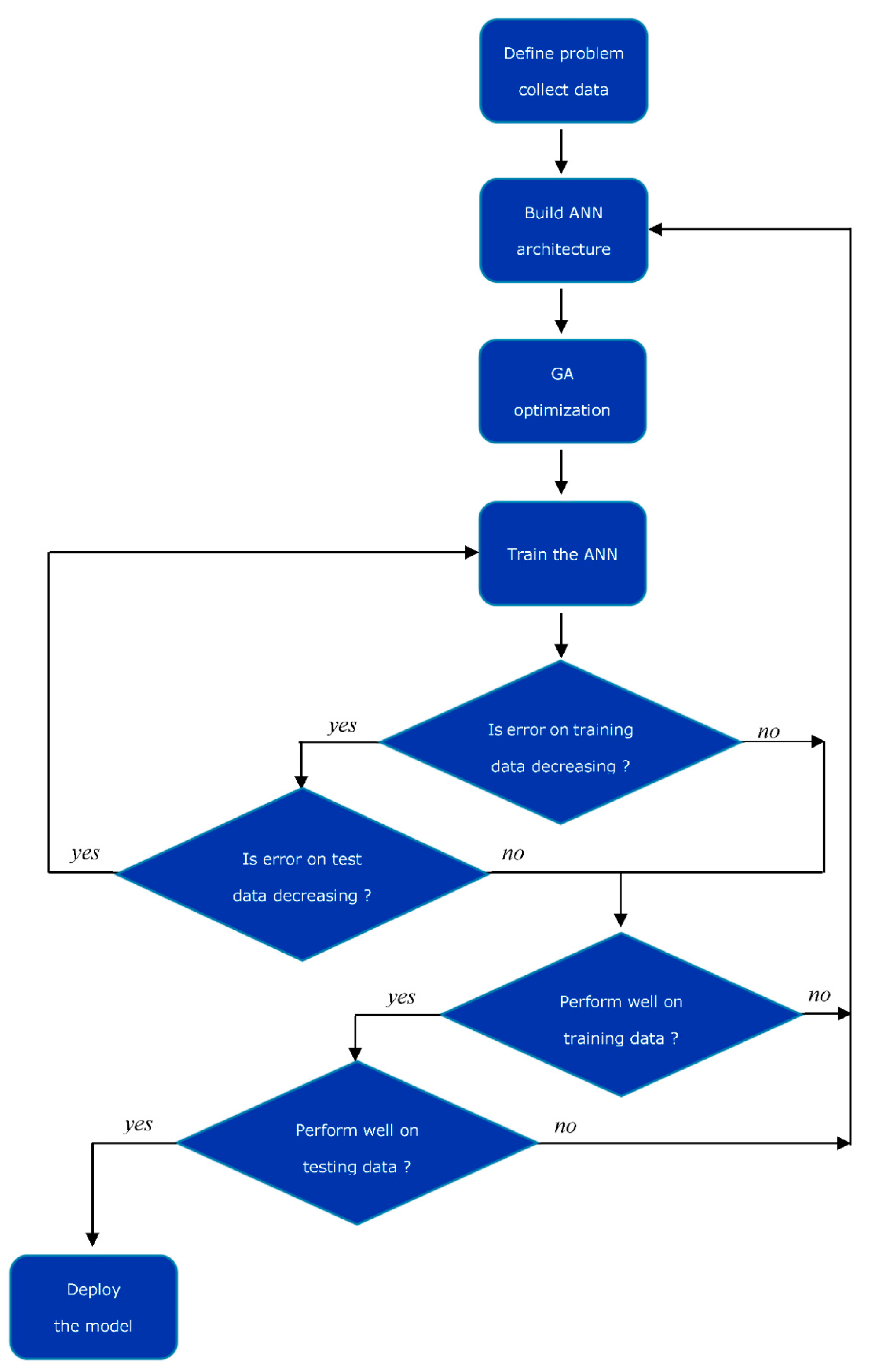
2.2. The Bio-Inspired Optimization Methods

The NeuroNet application by Mic-Apps Limited was used to develop the AGENN model. It is a tool for managing and optimizing artificial Neural Networks via techniques used by Genetic Algorithms [59,73]. These two methods belong to the so-called biologically motivated computing approaches as the biology systems delivered inspiration for the development of such computational systems [74].

The whole model’s development procedure consists of two main steps (Figure 3).

During the first one, the parameters of a beforehand determined Neural Network are selected and optimized via the Genetic Algorithms (GA). In this epoch, the region of a global optimum is located by reproduction, cross-over, and mutations techniques.

In the next stage, the training of the ANN via the backpropagation (BP) method is carried out. In this phase, the ANN’s parameters are refined, allowing to improve the performance and accuracy of the model [75].

A detailed description of the mathematical model behind the software can be found in the subsequent sections as well as in Appendix A.

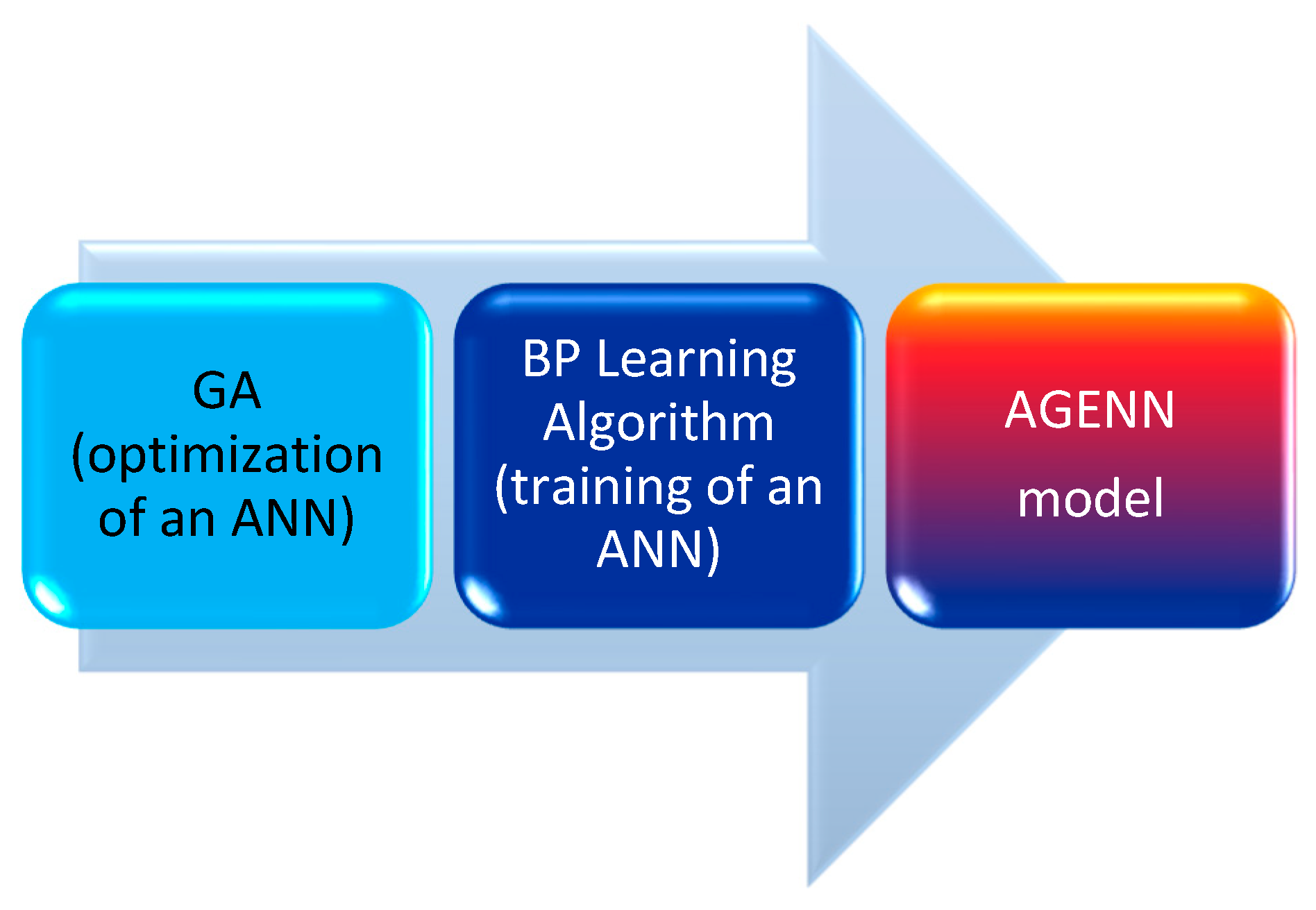
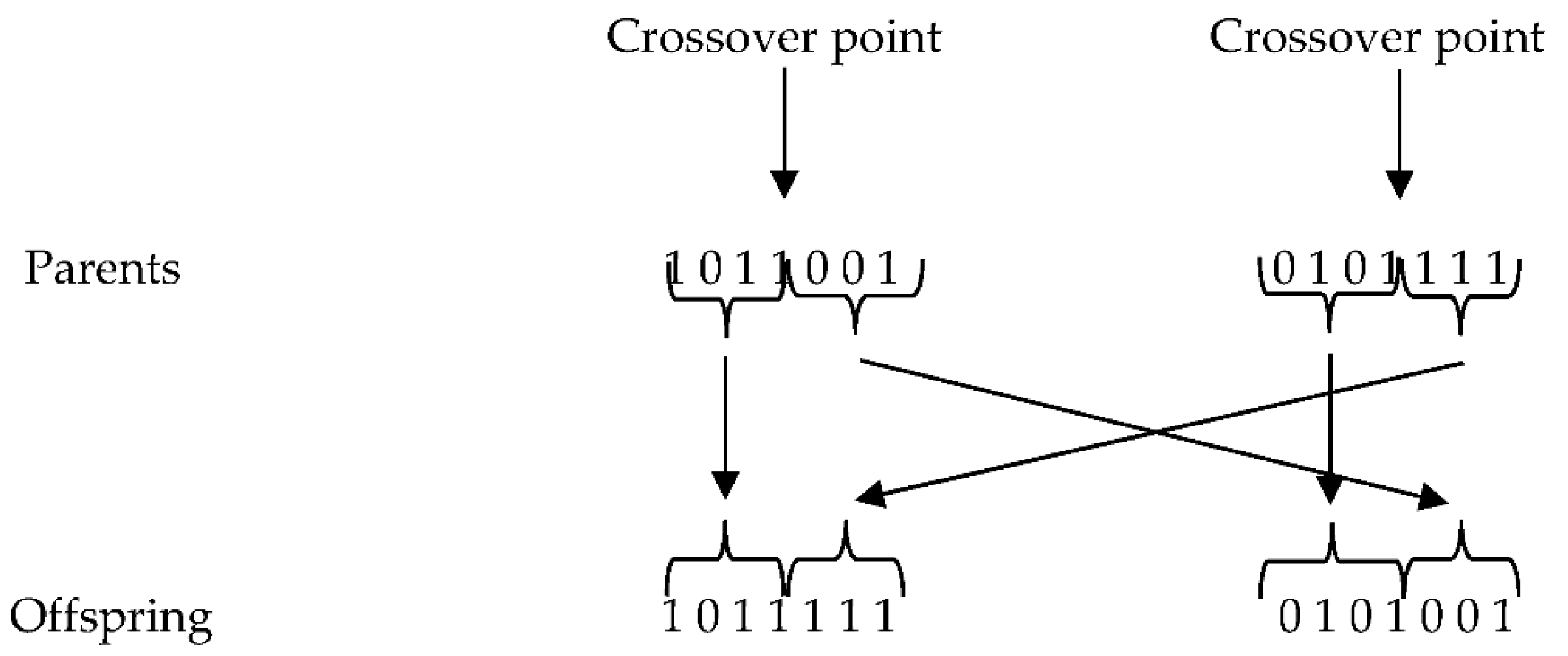
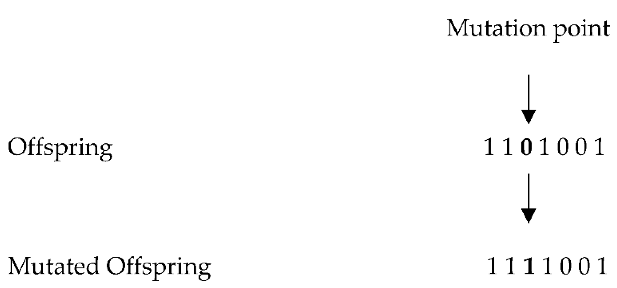
2.2.1. Genetic Algorithms Approach

Numerous parameters of a Genetic Algorithm ought to be previously set and adjusted before we start to develop the model. The most crucial GA model’s factors are: maximum number of iterations (n_iter), maximum storage (n_s), population size (n_pop), reseed fraction (r_f), maximum number of reseed (n_r), screening offset (s_o), screening module (s_m), mutation factor (m_f), a nearest neighbor parameter (K_n), general control factor (GC_f), and the initial and final crowding factors (in_f and fin_f, respectively).

The maximum number of iterations constitutes the number of individuals, which are created before stopping the optimization, while the population size is the total of individuals that make the working set. The maximum storage is the number of individuals who are kept in memory as a reference, for producing new ones or during reseeding a young population. These individuals are also used in the cases when the working population loses its diversity and ought to be refreshed by the introduction of new individuals, to find the global optimum. A factor called reseed fractions states the fraction of the population that is reseeded, while the maximum number of reseeding parameter expresses the maximum amount of times a reseed possible during calculations.

Turning on the screening module helps to avoid calculating individuals who are too similar. An important parameter, called the mutation factor, expresses to what extent an individual is mutated. The other two ones, i.e., GC factor and K nearest neighbor, define how unlikely individuals are crossed together and determines the number of most adjacent specimens that are taken into account before rejection or screening, respectively. To maintain the variety inside a population and help the exploration process, the initial crowding factor has to be close to, or equal 1, while the final one ought to be close to or just equal 0, to eliminate the diversity among individuals.

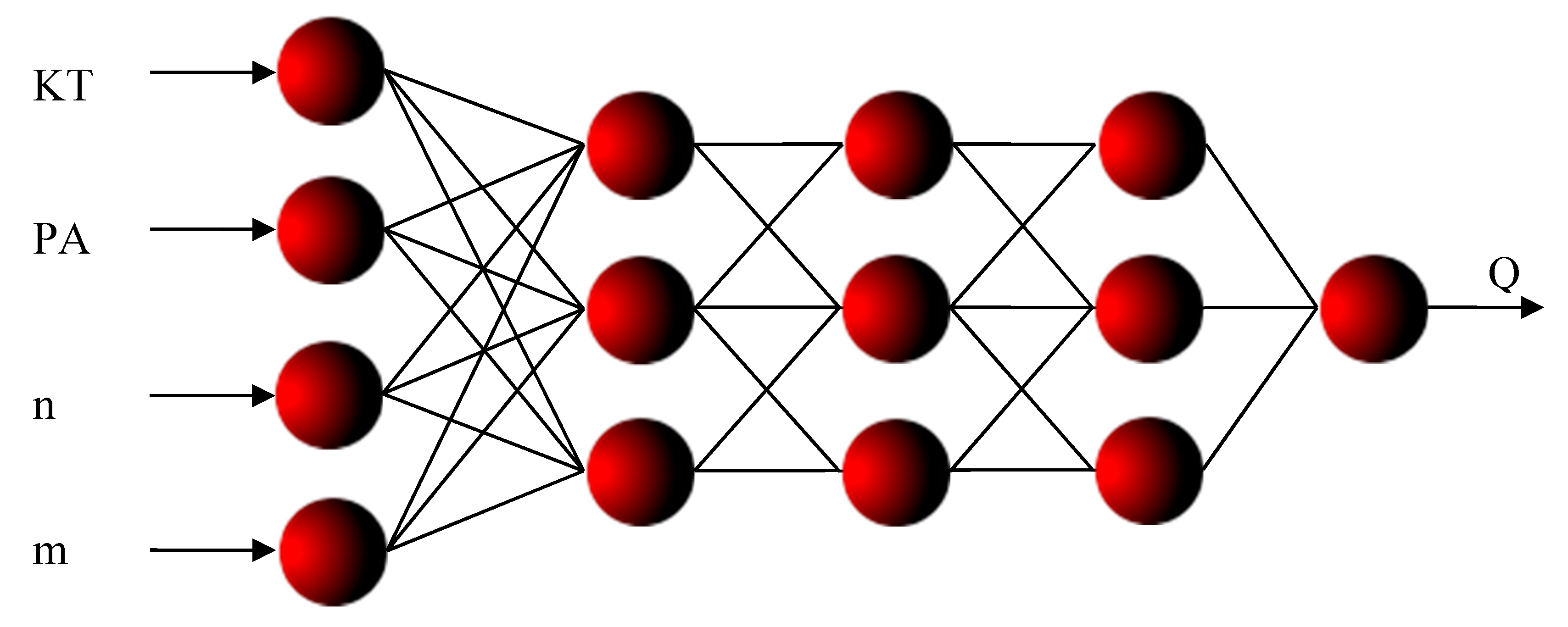
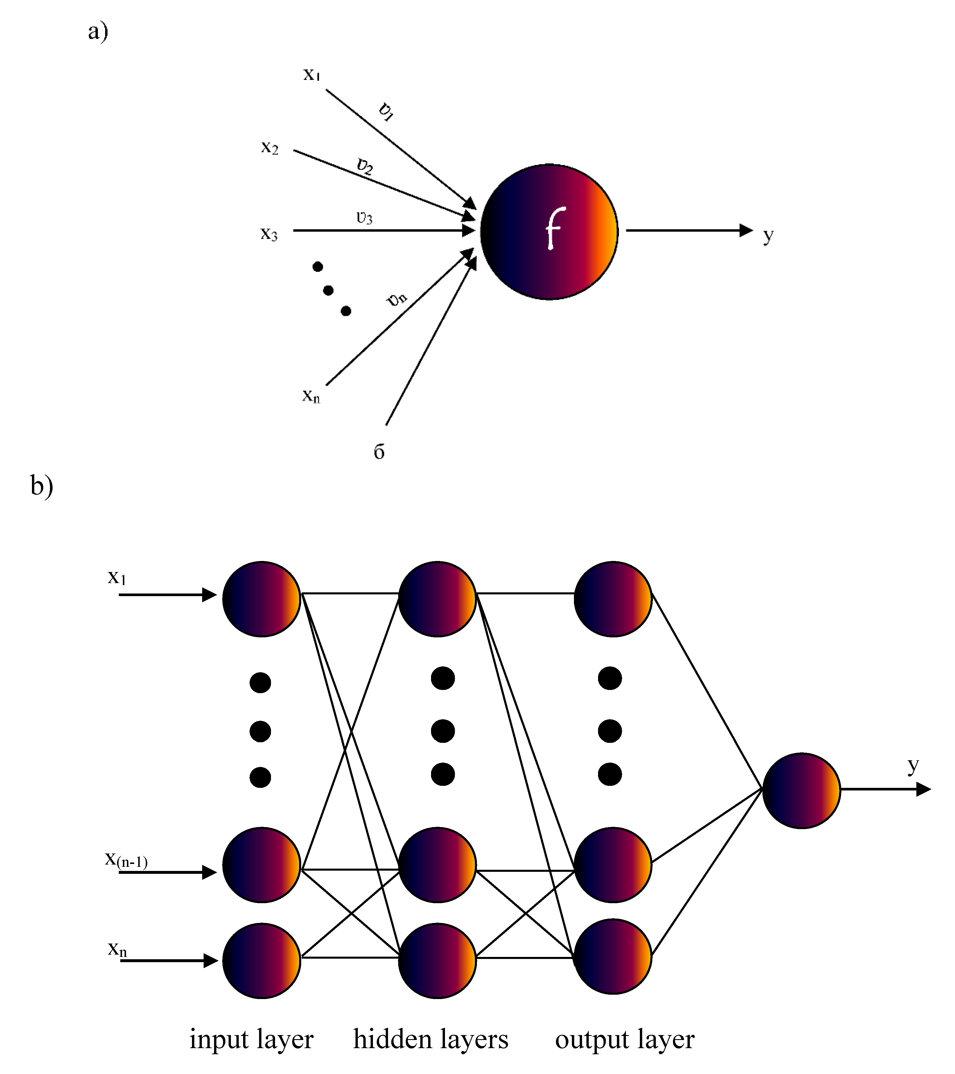
2.2.2. Neurocomputing Approach

The second stage of the model’s performance procedure constitutes using a gradient descent method via the BP scheme (Figure 3). The applied method is based on the ANN’s ability to reproduce an object or a process from training data. Moreover, Artificial Neural Networks are capable of dealing with ill-defined, uncertain, incomplete, and imprecise, redundant, and excess data as well as generalizing the complex interactions between inputs and outputs. Such kinds of data are usually a feature of a complex system. During the BP scheme, simultaneous modification of momentum, as well as the learning rate is conducted, since they are crucial parameters, significantly influencing the learning capability of an ANN model.

The learning rate defines the training rate of a network, while momentum describes the inertia of the learning process. Higher values of learning rates may lead to a lack of convergence and cause an overlook of the optimum. On the other side, for the lower learning rates, the training process may stack in a local optimum, instead of the global one [59]. Momentum allows ignoring insignificant features of the training data set, but higher values permit to obtain the solution faster. Too high ones, however, usually lead to instability of the whole training process.

This approach turned out to be a very effective method, as the formulated AGENN model is capable of making accurate predictions being developed on limited training data. For the purpose of this paper, the data given in [38] were used to derive and validate model parameters. The set of the desired data consists of a total of 88 samples with 18 independent testing results. Therefore, learning examples stand for the data set of 70 input-output data pairs, acquired from the operation of the large falling film evaporator. These results cover different design (geometric configuration) inputs and a wide range of operating conditions, including various kinds of tubes (plain and three kinds of enhanced tubes: Turbo B, Turbo BII and Turbo EHP) different tube pass arrangements (top-to-bottom, side-by-side and bottom-to-top), as well as broad range of liquid refrigerant mass flow rates and number of flooded tubes of the evaporator [38].

Since the developed approach is based on the AI methods using Genetic Algorithms and neurocomputing techniques, detailed heat transfer calculations of a heat exchanger are not necessary to be carried out. That is why the proposed approach can be considered as a complementary method and alternative task in a heat exchanger design procedure, besides the common rating and sizing tasks, which are based on thermal analysis with sizing (design problem) and rating (performance analysis) calculations.

Moreover, the proposed method is flexible in the use and provides novel abilities to optimize the design and performance of heat exchangers. A more detailed description of the approach can be found in the Appendix A.

For the considered case, a proper selection of the inputs allows determining optimum geometric configurations and operating conditions to obtain the required total heat transfer rate of a heat exchanger, e.g., the large evaporator. This is where the neurocomputing approach can sometimes overcome the shortcomings of expensive experimental procedures, as well as the laborious, conventional programmed computing approach, and also stands for the novelty of the paper.

The next section shows the application of the method and the developed model.

3. Results and Discussion

3.1. Application of the Method

As was previously underlined, an ANN operation depends on its topology, including the number of layers and neurons in each layer, where the number of input and output neurons is equal to the number of inputs and outputs, respectively. Therefore, the first phase in the whole model’s performance process, i.e., GA adjusting and optimization, when the main parameters of the ANN’s architecture are being set, is essential. The established GA model’s features are listed in

Table 2. The GA model’s parameters.

Parameter	Value
niter	1500
npop	33
ns	333
rf	1
nr	2
sm	On
so	1
mf	5
GCf	0.25
Kn	2
inf	1
finf	0.1

.

The second stage deals with Neural Network Optimization. The following factors are taken into account: the tag KT expressing the kind of tube (‘1′ for plain tubes, ‘2′ for Turbo B, ‘3′ for Turbo BII and ‘4′ for Turbo EHP tubes), the tag PA, which defines the tube passes arrangement (‘1′ for side-by-side (right to left or left to right), ‘2′ for top-to-bottom (the tube-side inlet pass at the top and the outlet at the bottom), ‘3′ for bottom-to-top), number n of flooded heat transfer tube rows and liquid refrigerant mass flow rate m to the top row of the tube array.

The inputs are listed in

Table 3. The inputs employed for training and testing of the AGENN model.

Input Parameter	Value
Kind of tubes, KT *	1, 2, 3, 4
Tube pass arrangement, PA **	1, 2, 3
Number of flooded heat transfer tube rows, n	1, 2, 3, 4, 5, 6, 7, 8
Liquid refrigerant mass flow rate, m, kg/s	4.5–12

* 1 stands for plain tubes, 2—Turbo B tubes, 3—Turbo BII tubes, 4—Turbo EHP tubes, ** 1 stands for side-by-side tube passes arrangement (right-to-left or left-to-right) tube, 2—Top-to-bottom, 3—Bottom-to-top.

.

An extended heat surface contains fins or appendages on primary heat transfer surfaces, leading to the increase in heat transfer area (usually on the gas side). Therefore, the performance of heat exchangers with enhanced tubes is higher than the one with plain tubes.

The tube pass arrangement defines the decline rates of the temperature difference between the refrigerant and chilled water along the tubes, which are different for different tubes pass arrangements. This decline leads to a decrease in the heat flux from the chilled water to the refrigerant and the reduction in the total heat transfer rate. On the other hand, the small refrigerant mass flow rate takes part in dry areas formation on the external tube surface. If the refrigerant flow rate is insufficient locally on the tube surface and the tube temperature is high enough, the local dry areas appear on the tube surface. This reduction of the effective wetted area by the liquid film on the tube surface deteriorates the overall heat transfer coefficient.

Finally, the number of flooded tube rows defines the number of tubes that should be flooded by the liquid refrigerant to keep the required amount of refrigerant at the bottom of the evaporator. This amount of coolant is necessary to recover the lubricant conveniently and keep the steady operation of the large evaporator.

The total heat transfer rate Q of the large falling film evaporator constitutes the output of the ANN model.

As the number of inputs and outputs define the total input and output neurons, the input and output layers are composed of 4 and 1 neurons, respectively.

The ANN of the developed AGENN model was trained using a supervised, BP training scheme [59].

Different ANN topologies were tested during the study, as the performance and the accuracy of the model depend on its architecture.

The number of hidden layers and neurons in each hidden layer was changing by one, and the performance of the AGEEN model was observed. The approach allows reducing the risk of memorization instead of generalization of the relationships within the considered data set. The optimal Neural Network turned out to be [4-3-3-3-1]. Three hidden layers with three sigmoid neurons in each of them form the developed AGENN model.

The architecture of the developed AGENN model is shown in Figure 4.

The logarithmic sigmoid function was applied as an activated function for all neurons. Such selection was made on the base of initial calculations, as well as prior experience and the fact that this kind of activation function is one of the widely used in the neurocomputing computations. The architecture of the considered [4-3-3-3-1] Artificial Neural Network is described in detail in

Table 4. The features of the AGENN model with [4-3-3-3-1] Artificial Neural Network.

Weights, υi,K,j *
υ0,0,0	−3.810
υ0,0,1	1.305
υ0,0,2	10.634
υ1,0,0	−10.013
υ1,0,1	−0.007
υ1,0,2	0.519
υ2,0,0	−2.125
υ2,0,1	0,859
υ2,0,2	3.013
υ3,0,0	−3.154
υ3,0,1	2.700
υ3,0,2	−9.283
υ0,1,0	−1.911
υ0,1,1	−4.618
υ0,1,2	2.567
υ1,1,0	9.920
υ1,1,1	7.640
υ1,1,2	−10.019
υ2,1,0	−4.603
υ2,1,1	1.021
υ2,1,2	2.377
υ0,2,0	−2.405
υ0,2,1	3.727
υ0,2,2	−8.748
υ1,2,0	−4.121
υ1,2,1	6.328
υ1,2,2	−10.000
υ2,2,0	−7.475
υ2,2,1	−3.965
υ2,2,2	−5.002
υ0,3,0	0.897
υ1,3,0	3.541
υ2,3,0	1.132
Neuron biases, бi,K *
б0,1	10.036
б1,1	2.755
б2,1	−7.759
б0,2	6.695
б1,2	1.904
б2,2	4.489
б0,2	−9.814
б1,2	−4.486
б2,2	6.041
б0,3	2.530

* a weight connecting the neuron i on a layer K with the neuron j on a layer K + 1; neurons and layers in the network in Figure 4 are numbered from top to bottom (i = 0–3), (j = 0–2) and from the left to the right (K = 0–3), respectively.

.

Since the knowledge about the influence of geometric and operational parameters on the total heat transfer rate of the heat exchanger is stored in the structure of the Artificial Neural Network, Table 4 summarizes essential data, including weights, obtained via the ANN’s training process, necessary stage to properly build of the considered AGENN model. So the data from Table 4 contain all the required information about the ANN topology, capable of describing the behavior of the considered heat exchanger, i.e., the large falling film evaporator.

An additional and valuable feature of the AGENN model is the possibility to conduct the advanced design considerations, using the non-integer values of KT and PA. These cases allow taking into account diverse tubes configurations, including shares of different kinds of tubes and tube pass arrangements within the evaporator’s construction. Moreover, the non-integer value of n means partially flooded tube rows. Thus, the presented approach allows considering various geometric and operational scenarios of the heat exchanger. Thus, the developed model is capable of generalizing the knowledge about the object gained during the learning stage, and this comprehensive tool provides unique abilities for design considerations and performance of a heat exchanger.

3.2. Validation of the Model

The AGENN model has been successfully validated against the desired data, both training and the new results, unseen by the network during the training process, since the comparison between desired and predicted data is considered as the most challenging method of validation. The comparison of the predicted Q_p and the desired Q_d total heat transfer rate of the evaporator, for wide range of both: geometric and operating conditions as well as different kinds of tubes, variety of tube pass arrangements, number of flooded heat transfer tube rows, and liquid refrigerant mass flow rates, is presented in Figure 5.

Good performance of the developed AGENN model has been achieved, even for the new testing data set. The predicted results are located within the range of ±3%, compared to the desired data. Such small relative error forms a solid basis for the possibility of using the developed model in practice.

The heat transfer rates of the considered large falling film evaporator, desired and predicted by the AGENN model with [4-3-3-3-1] Artificial Neural Network, are also shown in

Table 5. The selected values of heat transfer rate desired Q_d vs predicted Q_p by the AGENN model.

	Inputs, Outputs, Error	KT	PA	N	m	Qd	Qp	δ
Data		-	-	-	kg/s	kW		%
Data not used for training the ANN		4	2	5	10	1134.9	1137.8147	‒0.26
		4	3	5	5.12	1136.6	1134.3085	0.20
		4	1	3	5.75	1074.4	1076.1096	‒0.16
		4	1	6	5.75	1113.3	1106.7961	0.58
		4	2	4	5.75	1080.9	1089.7294	‒0.82
		4	3	2	5.75	1114.9	1120.3034	‒0.49
		4	3	7	5.75	1139.3	1138.4263	0.08
Data used for trainingthe ANN		1	1	5	5.75	425	433.977	‒2.11
		2	1	5	5.75	1051	1052.118	‒0.11
		3	1	5	5.75	1066	1063.146	0.27
		4	1	5	5.75	1105	1099.907	0.46
		4	2	5	5.75	1090	1099.704	‒0.89
		1	3	5	5.75	426	427.600	‒0.38
		2	3	5	5.75	1080	1063.684	1.51

.

The relative errors for most of the predicted Q are even smaller than 1%. The comparison of the desired and predicted heat transfer rate of the large falling film evaporator is also shown in Figure 6 and Figure 7. The higher errors are observed for lower heat transfer rates and liquid refrigerant mass flow rates. This behavior can be attributed to the difficulties in precisely determining the operational parameters in such conditions. For lower mass flow rates of liquid refrigerant to the top row of the tube array, dry patches in the first and the second tube rows may be generated, or even small maldistribution of liquid refrigerant may occur. Such conditions deteriorate the total heat transfer rate of the evaporator. Additionally, the nonlinear domain, which exists at low mass flow rates, ought to be covered by more training data, which are hardly available, especially for large-scale units. Nevertheless, the maximum error is lower than ±3%. The highest relative error of the prediction generated by the AGENN model is equal to 2.11%. This observation confirms the excellent generalization ability of the developed [4-3-3-3-1] type of ANN, which validates the broad applicability of the proposed approach and the developed AGENN model. The achieved results also confirmed that the developed AGENN model is flexible enough to be applied for different design configurations and a wide range of operational conditions.

Various kinds of tubes (plain and enhanced tubes: Turbo B, Turbo BII, and Turbo EHP), different tube pass arrangements (top-to-bottom, side-by-side, and bottom-to-top) as well as a wide range of liquid refrigerant mass flow rates and numbers of flooded tubes can be analyzed by the tool. Thus, the AGENN model can successfully determine the required design considerations and operating conditions to generate the desired total heat transfer rate of the large evaporator.

The introduced method allows getting quick and accurate results, as an answer to new inputs, via the non-iterative or end-to-end, easy to use, calculating procedure. In the considered case, one only has to enter the inputs: KT, PA, n, and m, to calculate the total heat transfer rate Q of the large-scale evaporator.

Such a developed tool allows also studying the influence of input variables on the evaporator’s total heat transfer rate. To conduct the study, other inputs ought to be fixed, as a dependency can be determined only for the specific case, expressed by geometric and operational conditions.

Such methodology was carried out, and the results are given in the next Section of the paper.

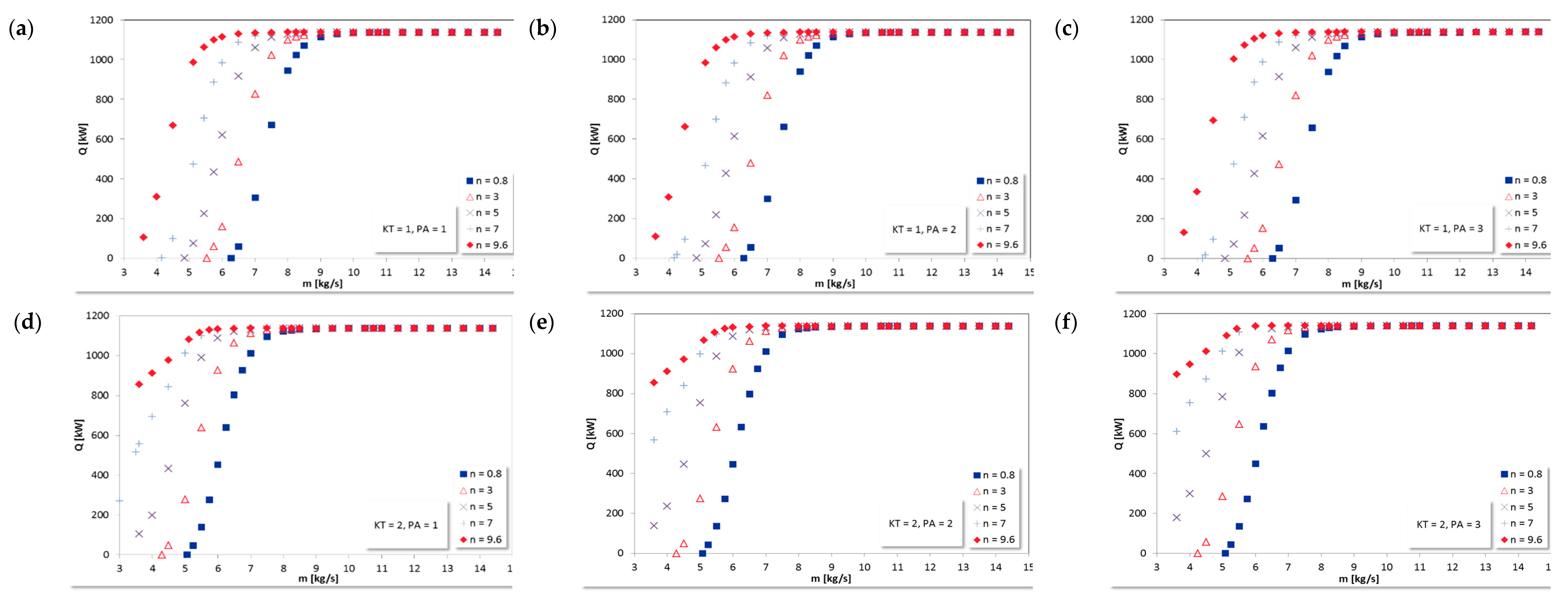
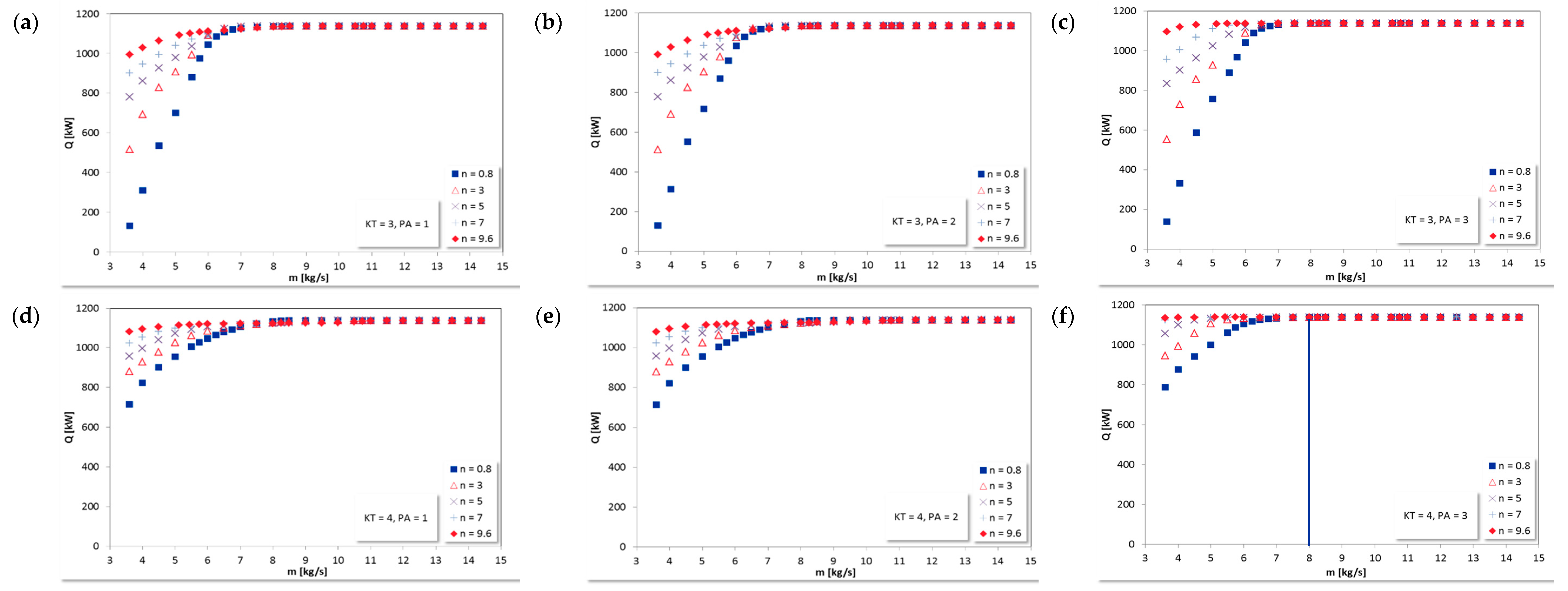
3.3. Effect of the Evaporator Design and Operating Parameters on the Heat Transfer Rate

To evaluate the impact of the inputs, i.e., the evaporator design and operating variables on the total heat transfer rate of the evaporator, the input parameters with values extended by 20% each way were applied to allow making predictions outside of the training zone. The basic structural configurations of the large falling film evaporator take into account four kinds of tubes and three types of pass arrangements, expressed by the integer KT and PA values, respectively.

However, as was mentioned before, in the specific, considered case, the developed AGENN model allows also finding more advanced design solutions of the evaporator. The non-integer values of KT and PA stand for sophisticated cases, corresponding to the mixed shares of different kinds of tubes and types of tube pass arrangements, respectively (

Table 6. The extended ranges of inputs used in the optimization study by AGENN model.

Input Parameter	Value
Kind of tubes, KT *	1–4
Tube pass arrangement, PA **	1–3
Number of flooded heat transfer tube rows, n	0.8–9.6
Liquid refrigerant mass flow rate, m, kg/s	3.6–14.4

* 1 stands for plain tubes, 2—Turbo B, 3—Turbo BII, 4—Turbo EHP, ** 1 stands for side-by-side tube passes arrangement (right to left or left to right) tube, 2—Top-to-bottom, 3—Bottom-to-top.

).

The non-integer n values express partially flooded heat transfer tube rows inside the large evaporator. Thus, the introduced method based on the neurocomputing approach and the developed AGENN model allows taking into account advanced structural configurations and operating scenarios of the heat exchanger.

This feature is an added value of the proposed approach allowing to evaluate nonstandard and complex cases, defined by a set of input data.

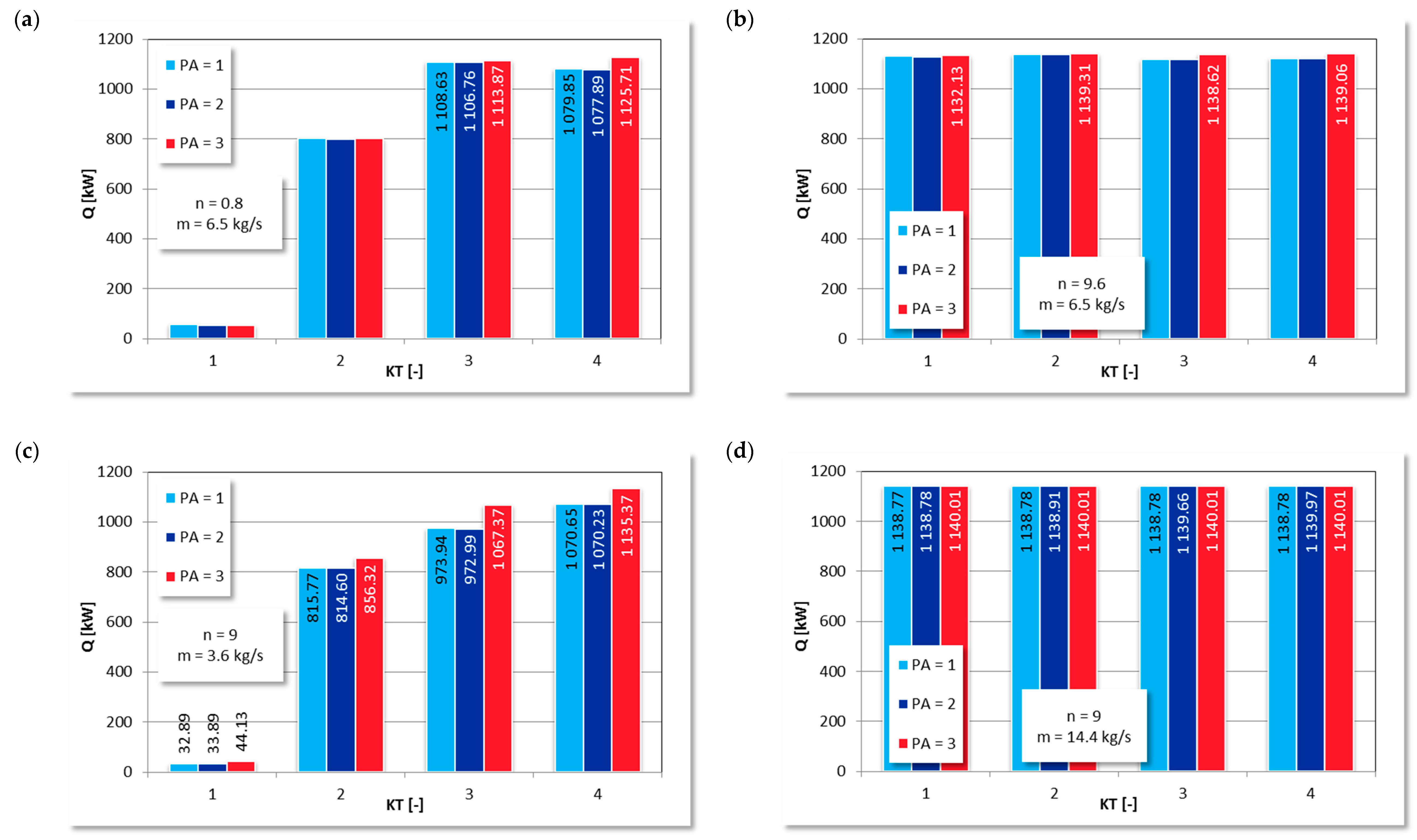
3.3.1. Effect of Kinds of Tubes and Tube Pass Arrangements

The influence of a type of tubes on the total heat transfer rate of the considered large falling film evaporator is given in Figure 8. The study was performed, including the lowest and the highest number of flooded heat transfer tube rows n, as well as liquid refrigerant mass flow rate m, respectively.

For the lowest n = 0.8, the liquid refrigerant mass flow rate should be higher than 6.27 kg/s to allow the reliable operation of the evaporator. Therefore, further considerations were performed for m = 6.5 kg/s (see the top row in Figure 8). On the other hand, for the lowest refrigerant mass flow rate, equal to 3.6 kg/s, the minimum number of fully flooded heat transfer tube rows corresponds to 9. That is why further analysis was performed for n = 9 (see the bottom row in Figure 8).

The obtained results revealed that the tubes with enhanced/augmented heat transfer surfaces (KT > 1) are more efficient and allow to generate higher heat transfer rates as the increase in surface area (e.g., in a finned surface) is one of the main methods to enhance the heat transfer rate. Even though the highest heat transfer rate Q_max = 1140.01 kW can be obtained for all kinds of tubes (Figure 8d), the most effective one seems to be the Turbo-EHP (Figure 8a,c). The lowest heat transfer rate was obtained for plain tubes (KT = 1), whereas the highest one for Turbo-EHP (KT = 4), characterized by a favorable combination of geometric parameters, including the highest, among enhanced tubes of both root and nominal inside diameters; thus, the following dependency can be written:

Q_{KT = 1} < Q_{KT = 2} < Q_{KT = 3} < Q_{KT = 4}

(4)

However, the increase in mass m flow rates of liquid refrigerant to the top row of the tube array and the number of flooded heat transfer tube rows n leads to the reduction in the significance of the kind of tubes KT parameter (Figure 6, Figure 7 and Figure 8). At the highest m = 14.4 kg/s, the evaporator reaches the highest heat transfer rate Q_max = 1140.01 kW (Figure 8d) for all kinds of tubes KT, but only for bottom-to-top tube pass arrangement (PA = 3). The PA significance also lowers with the increase of n and m (Figure 6 and Figure 7). However, for the lowest n = 0.8 (Figure 8a) and m = 3.6 kg/s (Figure 8c) the bottom-to-top tube pass arrangement (PA = 3) allows obtaining higher heat transfers rates.

The influence of tubes pass arrangements PA on Q is associated with the decline rates of the temperature difference between the refrigerant and chilled water along the tubes, which are different for different pass arrangements [39]. This decline leads to a decrease in the heat flux from the chilled water to the refrigerant and the reduction in the total heat transfer rate. For the optimum, bottom-to-top tube pass arrangement, only a few dry patches are created in the rows of falling film tubes, as this is the most effective tube pass arrangement with crossflow and counterflow of both fluids [1,2,4].

Operating parameters should also be taken into account to define the optimum operating strategy of the evaporator.

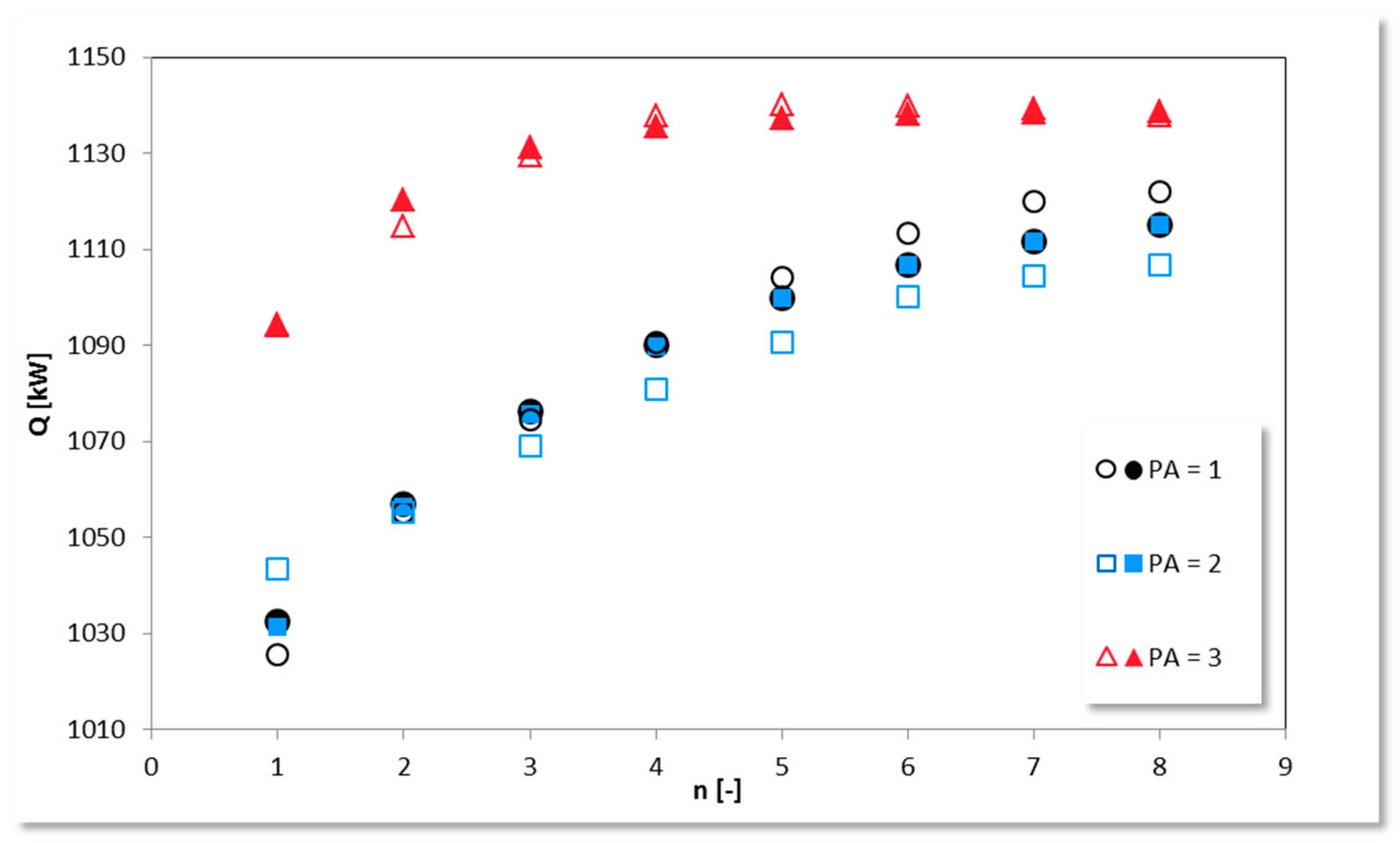
3.3.2. Effect of the Number of Flooded Tube Rows and the Refrigerant Mass Flow Rates

To easily recover lubricant and keep a well overall performance in varied loads, usually, several bottom tubes are flooded in the falling film evaporators. The rest, upper heat transfer tube rows, are wetted by the liquid refrigerant film from the trickling distributor, making so-called falling film tubes [38].

In other words, the number of flooded tube rows defines the number of tubes that should be flooded by the liquid refrigerant to keep the required amount of refrigerant at the bottom of the evaporator. This amount of refrigerant is necessary to recover the lubricant conveniently and keep the steady operation of the large evaporator.

However, for a higher number of flooded heat transfer tube rows, the lower tubes exhibit poor heat transfer performance as the negative influence of the liquid refrigerant column on the evaporation appears. Thus, the optimum n depends on the specific both design and operational conditions, including the refrigerant mass flow rate m [76].

The influence of mass flow rates m and the number n of flooded tube rows on the total heat transfer rate of the evaporator are given in Figure 9 and Figure 10. The increase in mass flow rates m of liquid refrigerant to the top row of the tube array leads to the rise in the heat transfer rate Q of the evaporator. Such behavior can be explained by the fact, that for high enough m, more heat evaporation can be withdrawn from the tubes system with the evaporated steam. In such conditions, the number of local dry areas on the tubes surfaces decreases and the falling film mode between horizontal tubes changes from droplet mode, through the jet mode, where liquid leaves the tube as continuous columns, to the sheet mode [35].

On the other hand, the local dry areas appear on the tubes surfaces for locally insufficient refrigerant liquid flows and high enough tube’s surface temperature, due to the reduction of the active wetted area by the liquid film. Such conditions may occur, especially for the lower tubes (counting from the top tube rows) placed under the refrigerant distributor. Since at dry areas heat transfer happens only via natural convection, the lower liquid mass flow rates lead to the deterioration of the overall external heat transfer performance [77].

The total heat transfer rate of the evaporator increases with m before the flow rate reaches a certain value, and then, it is kept almost constant. These transition values are different for various kinds of tubes KT, tube pass arrangements PA and number n of flooded tubes in the evaporator. Generally, it declines with the increase in input parameters KT, PA, n, and almost disappears for KT = 4, PA = 3, n > 7.

The reported above observations allow selecting the best operational strategy of the evaporator, which is depicted in the next section.

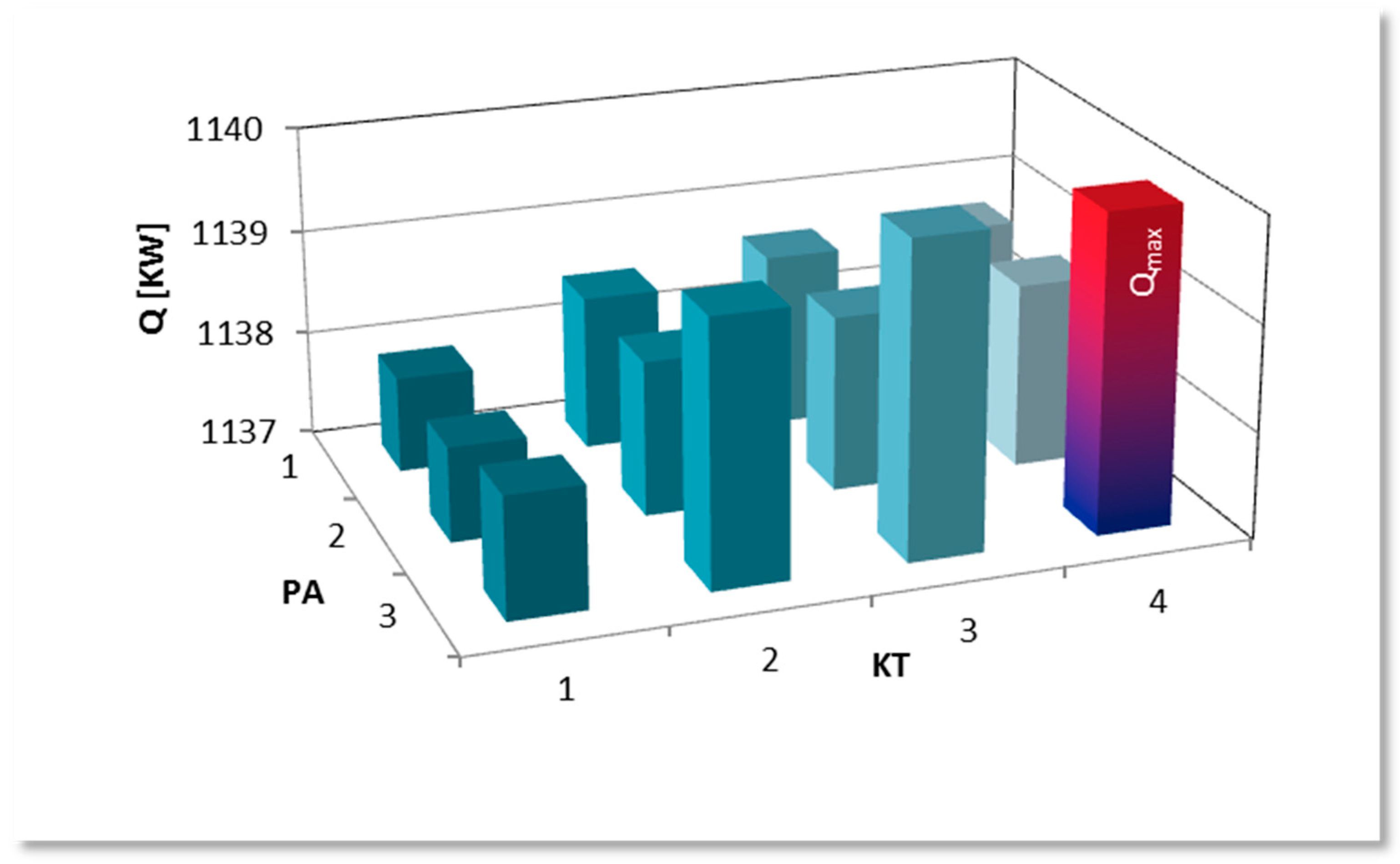
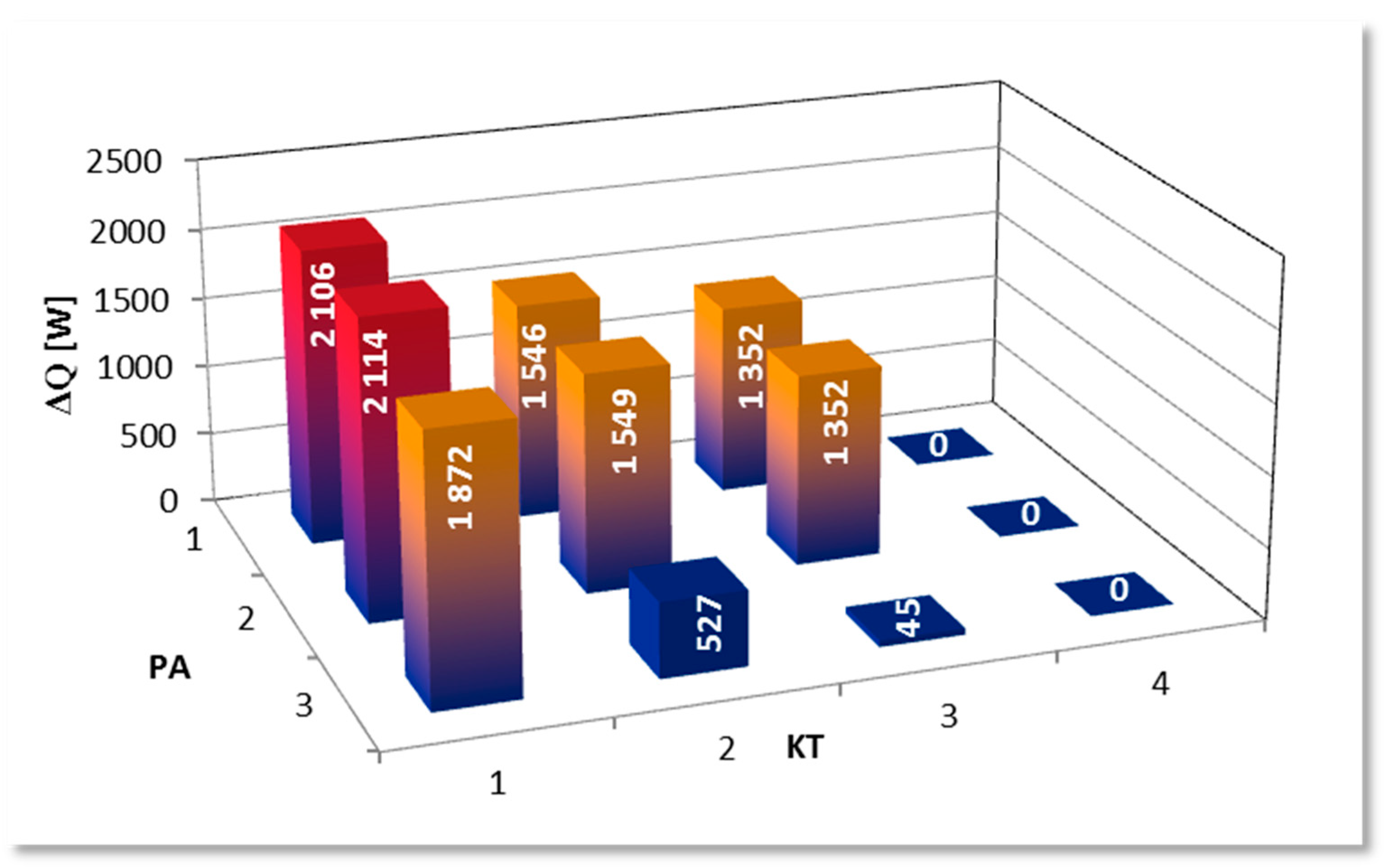
4. The Best Strategy for Heat Transfer Efficiency of the Evaporator

The evaluation carried out in this study showed, that the total heat transfer rate, i.e., the heat transfer efficiency of the evaporator, depends on the kind of tubes (KT), the tube pass arrangement (PA), the number of flooded tube rows (n) and the refrigerant mass flow rate (m). The developed global AGENN model, based on the introduced AI approach, allows to optimize the heat exchanger as the optimal set of input parameters could be determined, taking into account the total heat transfer rate i.e., the output value. In the case of the considered large falling film evaporator, some structural and operational parameters can be selected, defining the optimal design of the evaporator and the best strategy in thermal energy conversion.

As was underlined above, the highest total heat transfer rate is equal to Q_max = 1140.01 kW and can be obtained for all kinds of tubes, but only for bottom-to-top tube pass arrangement (PA = 3) and the selected optimal operational conditions n and m (Figure 8). However, to minimize operational costs and the negative effect of the hydrostatic pressure of the refrigerant, the n and m should be reduced [30,31,32]. The developed AGENN model allows selecting the optimal mass flow rate of the refrigerant, corresponding to the minimum value n = 0.8 of flooded tubes for each kind of tubes KT, allowing to obtain Q_max. The results confirm previous observations that the most effective type of tube is the KT = 4, i.e., the Turbo-EHP, as the lowest refrigerant mass flow rate is demanded, equal to 8 kg/s (Figure 10f).

Thus, the highest total heat transfer rate Q_max can be achieved by the large falling film evaporator for the structural configurations and operating scenarios, described by the following input parameters: KT = 4, PA = 3, n = 0.8 and m = 8 kg/s (Figure 11).

Taking into account the fact that the highest heat transfer efficiency of the evaporator can be achieved for the extended Turbo-EHP kind of tubes (KT = 4), we can determine the increase in the total heat transfer rate ΔQ, relative to that which can be obtained for other kinds of tubes (KT = 1, 2, 3). The results can be seen in Figure 12.

The highest increase in the total heat transfer rate is observed when the Plain tubes (KT = 1) are replaced with the Turbo EHP ones (KT = 4). The results are also confirmed by the effectiveness ε of the falling film evaporator. From all the considered structural and operational sceneries, the highest effectiveness is equal to ε = 0.866, which corresponds to the selected optimum case.

Finally, the cost of the heat exchanger should be a further criterion of the heat exchanger selection in the introduced approach.

It is also worth mentioning that a critical issue turns out to be a reliable operation of liquid refrigerant distributors. Trickling distribution of refrigerants in falling film evaporators are more effective than spraying one and saves the recycle pump. As was underlined above, if the mass flow rate of falling refrigerant is not equal to the evaporated one or if the refrigerant is not evenly distributed onto the first row of the tube bundles, the maldistribution of liquid occurs and dry out areas on local surfaces may be formed, leading to the deterioration of the total heat transfer rate of the evaporator [39].

The developed AGENN model allows optimizing both geometrical and operational indicators of heat exchangers, including large falling film evaporators. The introduced bio-inspired technique may also be treated as a convenient tool for rapid and virtual prototyping environments described by Rix et al. [78] of heat exchangers, as it allows to extend the approach to a more general problem from design considerations to sizing and rating ones. The proposed method can be considered as a complementary task in a heat exchanger design procedure.

5. Conclusions

The paper introduces a comprehensive, innovative bio-inspired approach in heat exchangers optimization, using AI methods. The application of the method was illustrated on a large falling-film evaporator, as one the most promising evaporators in renewable, adsorption desalination-cooling systems.

The AGENN model is developed in the paper using Genetic Algorithms and Neural Networks. The model allows conducting an optimization study of the heat exchanger concerning the total heat transfer rate of the evaporator. Good agreement between predicted and desired data was achieved. A maximum relative error, lower than ±3%, validates the reliability of the model. The highest total heat transfer rate, which can be obtained by the evaporator, is 1140.01 kW and may be achieved for Turbo EHP tubes, bottom-to-top tubes pass arrangements, the minimum number of flooded tube rows and liquid refrigerant mass flow rate 8 kg/s.

The introduced AI approach, which belongs to the soft computing techniques, can be considered as an alternative and complementary method in heat exchangers design procedures, besides the common rating and sizing tasks.

Moreover, as the proposed technique allows us to derive critical parameters related to both design and operating conditions, from training samples and have the ability to generalize the acquired knowledge, it can be applied for all kinds of heat exchangers and refrigerants.

Thus, the method can be considered as a cost-effective and universal methodology that users, including process engineers, energy researchers, or environmental scientists, can apply to develop robustness AI-based models. Finally, the method can be treated as a tool for rapid and virtual prototyping environments and computer applications of heat exchangers.

References

1. Lienhard, J.H. A Heat Transfer Textbook, 4th ed.; Phlogiston Press: Cambridge, MA, USA, 2016; ISBN 978-0-486-31837-0. [Google Scholar]
2. Kakaç, S.; Liu, H.; Pramuanjaroenkij, A. Heat Exchangers: Selection, Rating, and Thermal Design, 3rd ed.; CRC Press: Boca Raton, FL, USA, 2012; ISBN 978-1-4665-5616-4. [Google Scholar]
3. Shah, R.K.; Sekulic, D.P. Fundamentals of Heat Exchanger Design; John Wiley & Sons: Hoboken, NJ, USA, 2003; ISBN 978-0-471-32171-2. [Google Scholar]
4. Cengel, Y.A.; Ghajar Afshin, J. Heat and Mass Transfer. Fundamentals & Application, 5th ed.; McGraw-Hill Education: New York, NY, USA, 2015. [Google Scholar]
5. Cengel, Y.A. Heat transfer. A Practical Approach, 2nd ed.; International Edition; Mc-Graw-Hill: New York, NY, USA, 2003. [Google Scholar]
6. Al-Zareer, M.; Dincer, I.; Rosen, M.A. A novel approach for performance improvement of liquid to vapor based battery cooling systems. Energy Convers. Manag. 2019, 187, 191–204. [Google Scholar] [CrossRef]
7. Choudhury, B.; Saha, B.B.; Chatterjee, P.K.; Sarkar, J.P. An overview of developments in adsorption refrigeration systems towards a sustainable way of cooling. Appl. Energy 2013, 104, 554–567. [Google Scholar] [CrossRef]
8. Kishore, R.A.; Davis, B.; Greathouse, J.; Hannon, A.; Kennedy, D.E.; Millar, A.; Mittel, D.; Nozariasbmarz, A.; Kang, M.G.; Kang, H.B.; et al. Energy scavenging from ultra-low temperature gradients. Energy Environ. Sci. 2019, 12, 1008–1018. [Google Scholar] [CrossRef]
9. Zhang, F.; Liu, J.; Yang, W.; Logan, E.B. A thermally regenerative ammonia-based battery for efficient harvesting of low-grade thermal energy as electrical power. Energy Environ. Sci. 2015, 8, 343–349. [Google Scholar] [CrossRef]
10. Marschewski, J.; Brenner, L.; Ebejer, N.; Ruch, P.; Michel, B.; Poulikakos, D. 3D-printed fluidic networks for high-power-density heat-managing miniaturized redox flow batteries. Energy Environ. Sci. 2017, 10, 780–787. [Google Scholar] [CrossRef]
11. Wang, R.Z.; Xia, Z.Z.; Wang, L.W.; Lu, Z.S.; Li, S.L.; Li, T.X.; Wu, J.Y.; He, S. Heat transfer design in adsorption refrigeration systems for efficient use of low-grade thermal energy. Energy 2011, 36, 5425–5439. [Google Scholar] [CrossRef]
12. Li, X.H.; Hou, X.H.; Zhang, X.; Yuan, Z.X. A review on development of adsorption cooling—Novel beds and advanced cycles. Energy Convers. Manag. 2015, 94, 221–232. [Google Scholar] [CrossRef]
13. Garg, P.; Orosz, M.S. Economic optimization of Organic Rankine cycle with pure fluids and mixtures for waste heat and solar applications using particle swarm optimization method. Energy Convers. Manag. 2018, 165, 649–668. [Google Scholar] [CrossRef]
14. Bowman, R.A.; Mueller, A.C.; Nagle, W.M. Mean temperature difference in design. Trans. ASME 1940, 62, 283–294. [Google Scholar]
15. Sanaye, S.; Hajabdollahi, H. Thermal-economic multi-objective optimization of plate fin heat exchanger using genetic algorithm. Appl. Energy 2010, 87, 1893–1902. [Google Scholar] [CrossRef]
16. de Souza-Santos, M.L. Proposals for power generation based on processes consuming biomass-glycerol slurries. Energy 2017, 120, 959–974. [Google Scholar] [CrossRef]
17. Blaszczuk, A.; Nowak, W.; Krzywanski, J. Effect of bed particle size on heat transfer between fluidized bed of group b particles and vertical rifled tubes. Powder Technol. 2017, 316, 111–122. [Google Scholar] [CrossRef]
18. Błaszczuk, A.; Krzywański, J. A comparison of fuzzy logic and cluster renewal approaches for heat transfer modeling in a 1296 t/h CFB boiler with low level of flue gas recirculation. Arch. Thermodyn. 2017, 38, 91–122. [Google Scholar] [CrossRef]
19. Muskała, W.; Krzywański, J.; Rajczyk, R.; Cecerko, M.; Kierzkowski, B.; Nowak, W.; Gajewski, W. Investigation of erosion in CFB boilers. Rynek Energii 2010, 87, 97–102. [Google Scholar]
20. Muskała, W.; Krzywański, J.; Sekret, R.; Nowak, W. Model research of coal combustion in circulating fluidized bed boilers. Chem. Process Eng. Inz. Chem. I Proces. 2008, 29, 473–492. [Google Scholar]
21. Zylka, A.; Krzywanski, J.; Czakiert, T.; Idziak, K.; Sosnowski, M.; Grabowska, K.; Prauzner, T.; Nowak, W. The 4th Generation of CeSFaMB in numerical simulations for CuO-based oxygen carrier in CLC system. Fuel 2019, 255, 115776. [Google Scholar] [CrossRef]
22. Ceribeli, K.B.; de Souza-Santos, M.L. Effect of dry-solid content level in feeding slurry of municipal solid waste consumed by FSIG/GT power generation process; a theoretical study. Fuel 2019, 254, 115727. [Google Scholar] [CrossRef]
23. Markides, C.N.; Smith, T.C.B. A dynamic model for the efficiency optimization of an oscillatory low grade heat engine. Energy 2011, 36, 6967–6980. [Google Scholar] [CrossRef]
24. Solanki, R.; Mathie, R.; Galindo, A.; Markides, C.N. Modelling of a two-phase thermofluidic oscillator for low-grade heat utilisation: Accounting for irreversible thermal losses. Appl. Energy 2013, 106, 337–354. [Google Scholar] [CrossRef]
25. Sah, R.P.; Choudhury, B.; Das, R.K.; Sur, A. An overview of modelling techniques employed for performance simulation of low–grade heat operated adsorption cooling systems. Renew. Sustain. Energy Rev. 2017, 74, 364–376. [Google Scholar] [CrossRef]
26. Aristov, Y.I.; Glaznev, I.S.; Girnik, I.S. Optimization of adsorption dynamics in adsorptive chillers: Loose grains configuration. Energy 2012, 46, 484–492. [Google Scholar] [CrossRef]
27. Chorowski, M.; Pyrka, P. Modelling and experimental investigation of an adsorption chiller using low-temperature heat from cogeneration. Energy 2015, 92, 221–229. [Google Scholar] [CrossRef]
28. Ocłoń, P.; Łopata, S. Study of the Effect of Fin-and-Tube Heat Exchanger Fouling on its Structural Performance. Heat Transf. Eng. 2018, 39, 1139–1155. [Google Scholar] [CrossRef]
29. Ji, W.-T.; Zhao, E.-T.; Zhao, C.-Y.; Zhang, H.; Tao, W.-Q. Falling film evaporation and nucleate pool boiling heat transfer of R134a on the same enhanced tube. Appl. Therm. Eng. 2019, 147, 113–121. [Google Scholar] [CrossRef]
30. Cheppudira Thimmaiah, P.; Sharafian, A.; Huttema, W.; Osterman, C.; Ismail, A.; Dhillon, A.; Bahrami, M. Performance of finned tubes used in low-pressure capillary-assisted evaporator of adsorption cooling system. Appl. Therm. Eng. 2016, 106, 371–380. [Google Scholar] [CrossRef]
31. Thimmaiah, P.C.; Sharafian, A.; Rouhani, M.; Huttema, W.; Bahrami, M. Evaluation of low-pressure flooded evaporator performance for adsorption chillers. Energy 2017, 122, 144–158. [Google Scholar] [CrossRef]
32. Cheppudira Thimmaiah, P.; Sharafian, A.; Huttema, W.; McCague, C.; Bahrami, M. Effects of capillary-assisted tubes with different fin geometries on the performance of a low-operating pressure evaporator for adsorption cooling system applications. Appl. Energy 2016, 171, 256–265. [Google Scholar] [CrossRef]
33. Shahzad, M.W.; Myat, A.; Chun, W.G.; Ng, K.C. Bubble-assisted film evaporation correlation for saline water at sub-atmospheric pressures in horizontal-tube evaporator. Appl. Therm. Eng. 2013, 50, 670–676. [Google Scholar] [CrossRef]
34. Jin, P.-H.; Zhao, C.-Y.; Ji, W.-T.; Tao, W.-Q. Experimental investigation of R410A and R32 falling film evaporation on horizontal enhanced tubes. Appl. Therm. Eng. 2018, 137, 739–748. [Google Scholar] [CrossRef]
35. Abed, A.M.; Alghoul, M.A.; Yazdi, M.H.; Al-Shamani, A.N.; Sopian, K. The role of enhancement techniques on heat and mass transfer characteristics of shell and tube spray evaporator: A detailed review. Appl. Therm. Eng. 2015, 75, 923–940. [Google Scholar] [CrossRef]
36. Zhao, C.-Y.; Ji, W.-T.; Jin, P.-H.; Tao, W.-Q. Heat transfer correlation of the falling film evaporation on a single horizontal smooth tube. Appl. Therm. Eng. 2016, 103, 177–186. [Google Scholar] [CrossRef]
37. Li, W.; Wu, X.-Y.; Luo, Z.; Yao, S.; Xu, J.-L. Heat transfer characteristics of falling film evaporation on horizontal tube arrays. Int. J. Heat Mass Transf. 2011, 54, 1986–1993. [Google Scholar] [CrossRef]
38. Yang, L.; Wang, W. The heat transfer performance of horizontal tube bundles in large falling film evaporators. Int. J. Refrig. 2011, 34, 303–316. [Google Scholar] [CrossRef]
39. Yang, L.; Song, X.; Xie, Y. Effect of the Dryout in Tube Bundles on the Heat Transfer Performance of Falling Film Evaporators. Procedia Eng. 2017, 205, 2176–2183. [Google Scholar] [CrossRef]
40. Hou, H.; Bi, Q.; Zhang, X. Numerical simulation and performance analysis of horizontal-tube falling-film evaporators in seawater desalination. Int. Commun. Heat Mass Transf. 2012, 39, 46–51. [Google Scholar] [CrossRef]
41. Wunder, F.; Enders, S.; Semiat, R. Numerical simulation of heat transfer in a horizontal falling film evaporator of multiple-effect distillation. Desalination 2017, 401, 206–229. [Google Scholar] [CrossRef]
42. Kharangate, C.R.; Mudawar, I. Review of computational studies on boiling and condensation. Int. J. Heat Mass Transf. 2017, 108, 1164–1196. [Google Scholar] [CrossRef]
43. Chen, J.; Zhang, R.; Niu, R. Numerical simulation of horizontal tube bundle falling film flow pattern transformation. Renew. Energy 2015, 73, 62–68. [Google Scholar] [CrossRef]
44. Ren, C.; Wan, Y. A new approach to the analysis of heat and mass transfer characteristics for laminar air flow inside vertical plate channels with falling water film evaporation. Int. J. Heat Mass Transf. 2016, 103, 1017–1028. [Google Scholar] [CrossRef]
45. Benim, A.C.; Chattopadhyay, H.; Nahavandi, A. Computational analysis of turbulent forced convection in a channel with a triangular prism. Int. J. Therm. Sci. 2011, 50, 1973–1983. [Google Scholar] [CrossRef]
46. Ocłoń, P.; Łopata, S.; Nowak, M.; Benim, A.C. Numerical Study on the Effect of Inner Tube Fouling on the Thermal Performance of High-Temperature Fin-and-Tube Heat Exchanger. Available online: https://www.researchgate.net/publication/268506448_Numerical_study_on_the_effect_of_inner_tube_fouling_on_the_thermal_performance_of_high-temperature_fin-and-tube_heat_exchanger (accessed on 13 February 2019).
47. Sosnowski, M.; Krzywanski, J.; Grabowska, K.; Gnatowska, R. Polyhedral meshing in numerical analysis of conjugate heat transfer. EPJ Web Conf. 2018, 180, 02096. [Google Scholar] [CrossRef]
48. Ocłoń, P.; Łopata, S.; Chłosta, K. Experimental and Numerical Investigation of Flow Distribution within the Heat Exchanger with Elliptical Tubes. Procedia Eng. 2016, 157, 428–435. [Google Scholar] [CrossRef] [Green Version]
49. Grabowska, K.; Sosnowski, M.; Krzywanski, J.; Sztekler, K.; Kalawa, W.; Zylka, A.; Nowak, W. Analysis of heat transfer in a coated bed of an adsorption chiller. MATEC Web Conf. 2018, 240, 01010. [Google Scholar] [CrossRef] [Green Version]
50. Grabowska, K.; Sosnowski, M.; Krzywanski, J.; Sztekler, K.; Kalawa, W.; Zylka, A.; Nowak, W. The Numerical Comparison of Heat Transfer in a Coated and Fixed Bed of an Adsorption Chiller. J. Therm. Sci. 2018, 27, 421–426. [Google Scholar] [CrossRef]
51. Shah, M.M. A correlation for heat transfer during boiling on bundles of horizontal plain and enhanced tubes. Int. J. Refrig. 2017, 78, 47–59. [Google Scholar] [CrossRef]
52. Krzywanski, J.; Wesolowska, M.; Blaszczuk, A.; Majchrzak, A.; Komorowski, M.; Nowak, W. The Non-Iterative Estimation of Bed-to-Wall Heat Transfer Coefficient in a CFBC by Fuzzy Logic Methods. Procedia Eng. 2016, 157, 66–71. [Google Scholar] [CrossRef] [Green Version]
53. Dang, T.; Nguyen, H.; Nguyen, G. Experimental Investigations for Fluid Flow Characteristics of Refrigerant R134a in a Microtubes Evaporator. In Proceedings of the 2018 4th International Conference on Green Technology and Sustainable Development (GTSD), Ho Chi Minh City, Vietnam, 23–24 November 2018; pp. 385–390. [Google Scholar]
54. Halon, T.; Pelinska-Olko, E.; Szyc, M.; Zajaczkowski, B. Predicting Performance of a District Heat Powered Adsorption Chiller by Means of an Artificial Neural Network. Energies 2019, 12, 3328. [Google Scholar] [CrossRef] [Green Version]
55. Kim, J.-H.; Seong, N.-C.; Choi, W. Modeling and Optimizing a Chiller System Using a Machine Learning Algorithm. Energies 2019, 12, 2860. [Google Scholar] [CrossRef] [Green Version]
56. Karami, A.; Rezaei, E.; Rahimi, M.; Zanjani, M. Artificial Neural Modeling of the Heat Transfer in an Air Cooled Heat Exchanger Equipped with Butterfly Inserts. Int. Energy J. 2012, 13, 21–28. [Google Scholar]
57. Amiri, A.; Karami, A.; Yousefi, T.; Zanjani, M. Artificial neural network to predict the natural convection from vertical and inclined arrays of horizontal cylinders. Pol. J. Chem. Technol. 2012, 14, 46–52. [Google Scholar] [CrossRef] [Green Version]
58. Lin, L.; Wang, X. Design for refrigerator evaporator superheat based on direct adaptive fuzzy controller. In Proceedings of the 2016 Chinese Control and Decision Conference (CCDC), Yinchuan, China, 28–30 May 2016; pp. 6297–6300. [Google Scholar]
59. Krzywanski, J.; Grabowska, K.; Herman, F.; Pyrka, P.; Sosnowski, M.; Prauzner, T.; Nowak, W. Optimization of a three-bed adsorption chiller by genetic algorithms and neural networks. Energy Convers. Manag. 2017, 153, 313–322. [Google Scholar] [CrossRef]
60. Shi, H.; Ma, T.; Chu, W.; Wang, Q. Optimization of inlet part of a microchannel ceramic heat exchanger using surrogate model coupled with genetic algorithm. Energy Convers. Manag. 2017, 149, 988–996. [Google Scholar] [CrossRef]
61. Darvish Damavandi, M.; Forouzanmehr, M.; Safikhani, H. Modeling and Pareto based multi-objective optimization of wavy fin-and-elliptical tube heat exchangers using CFD and NSGA-II algorithm. Appl. Therm. Eng. 2017, 111, 325–339. [Google Scholar] [CrossRef]
62. Chitgar, N.; Emadi, M.A.; Chitsaz, A.; Rosen, M.A. Investigation of a novel multigeneration system driven by a SOFC for electricity and fresh water production. Energy Convers. Manag. 2019, 196, 296–310. [Google Scholar] [CrossRef]
63. Yin, Q.; Du, W.-J.; Ji, X.-L.; Cheng, L. Optimization design and economic analyses of heat recovery exchangers on rotary kilns. Appl. Energy 2016, 180, 743–756. [Google Scholar] [CrossRef]
64. Yin, Q.; Du, W.-J.; Cheng, L. Optimization design of heat recovery systems on rotary kilns using genetic algorithms. Appl. Energy 2017, 202, 153–168. [Google Scholar] [CrossRef]
65. Dezan, D.J.; Salviano, L.O.; Yanagihara, J.I. Heat transfer enhancement and optimization of flat-tube multilouvered fin compact heat exchangers with delta-winglet vortex generators. Appl. Therm. Eng. 2016, 101, 576–591. [Google Scholar] [CrossRef]
66. Saldanha, W.H.; Soares, G.L.; Machado-Coelho, T.M.; dos Santos, E.D.; Ekel, P.I. Choosing the best evolutionary algorithm to optimize the multiobjective shell-and-tube heat exchanger design problem using PROMETHEE. Appl. Therm. Eng. 2017, 127, 1049–1061. [Google Scholar] [CrossRef]
67. Cartelle Barros, J.J.; Lara Coira, M.; de la Cruz López, M.P.; del Caño Gochi, A. Sustainability optimisation of shell and tube heat exchanger, using a new integrated methodology. J. Clean. Prod. 2018, 200, 552–567. [Google Scholar] [CrossRef]
68. Roy, U.; Pant, H.K.; Majumder, M. Detection of significant parameters for shell and tube heat exchanger using polynomial neural network approach. Vacuum 2019, 166, 399–404. [Google Scholar] [CrossRef]
69. Roy, U.; Majumder, M. Evaluating heat transfer analysis in heat exchanger using NN with IGWO algorithm. Vacuum 2019, 161, 186–193. [Google Scholar] [CrossRef]
70. Wang, X.; Zheng, N.; Liu, Z.; Liu, W. Numerical analysis and optimization study on shell-side performances of a shell and tube heat exchanger with staggered baffles. Int. J. Heat Mass Transf. 2018, 124, 247–259. [Google Scholar] [CrossRef]
71. Bahiraei, M.; Khosravi, R.; Heshmatian, S. Assessment and optimization of hydrothermal characteristics for a non-Newtonian nanofluid flow within miniaturized concentric-tube heat exchanger considering designer’s viewpoint. Appl. Therm. Eng. 2017, 123, 266–276. [Google Scholar] [CrossRef]
72. Salam, Z.; Ahmed, J.; Merugu, B.S. The application of soft computing methods for MPPT of PV system: A technological and status review. Appl. Energy 2013, 107, 135–148. [Google Scholar] [CrossRef]
73. Krzywanski, J.; Fan, H.; Feng, Y.; Shaikh, A.R.; Fang, M.; Wang, Q. Genetic algorithms and neural networks in optimization of sorbent enhanced H2 production in FB and CFB gasifiers. Energy Convers. Manag. 2018, 171, 1651–1661. [Google Scholar] [CrossRef]
74. Kar, A.K. Bio inspired computing—A review of algorithms and scope of applications. Expert Syst. Appl. 2016, 59, 20–32. [Google Scholar] [CrossRef]
75. Krzywanski, J. Modeling of Energy Systems with Fixed and Moving Porous Media by Artificial Intelligence Methods; University of Warmia and Mazury in Olsztyn: Olsztyn, Poland, 2018; ISBN 978-83-60493-05-2. [Google Scholar]
76. Zhao, C.-Y.; Ji, W.-T.; Jin, P.-H.; Zhong, Y.-J.; Tao, W.-Q. Experimental study of the local and average falling film evaporation coefficients in a horizontal enhanced tube bundle using R134a. Appl. Therm. Eng. 2018, 129, 502–511. [Google Scholar] [CrossRef]
77. Edalatpour, M.; Liu, L.; Jacobi, A.M.; Eid, K.F.; Sommers, A.D. Managing water on heat transfer surfaces: A critical review of techniques to modify surface wettability for applications with condensation or evaporation. Appl. Energy 2018, 222, 967–992. [Google Scholar] [CrossRef]
78. Rix, J.; Haas, S.; Teixeira, J. Virtual Prototyping: Virtual Environments and the Product Design Process; Springer: New York, NY, USA, 2016; ISBN 978-0-387-34904-6. [Google Scholar]
79. Patterson, J.; Gibson, A. Deep Learning: A Practitioner’s Approach; O’Reilly Media, Inc.: Sebastopol, CA, USA, 2017; ISBN 978-1-4919-1423-6. [Google Scholar]
80. Rutkowski, L. Computational Intelligence: Methods and Techniques; Springer Science & Business Media: Boston, NY, USA, 2008; ISBN 978-3-540-76288-1. [Google Scholar]
81. Krzywanski, J.; Grabowska, K.; Sosnowski, M.; Żyłka, A.; Sztekler, K.; Kalawa, W.; Wójcik, T.; Nowak, W. Modeling of a re-heat two-stage adsorption chiller by AI approach. MATEC Web Conf. 2018, 240, 05014. [Google Scholar] [CrossRef]
82. Krzywanski, J.; Grabowska, K.; Sosnowski, M.; Zylka, A.; Sztekler, K.; Kalawa, W.; Wójcik, T.; Nowak, W. An Adaptive Neuro-Fuzzy model of a Re-Heat Two-Stage Adsorption Chiller. Therm. Sci. 2019, 23, 1053–1063. [Google Scholar] [CrossRef] [Green Version]
Figure 1. The schematic diagram of the large falling film evaporator.
Energies 12 04441 g001
Figure 2. The schematic diagram of the tube pass arrangements of the falling film evaporator, (a) side-by-side, (b) bottom-to-top and top-to-bottom.
Energies 12 04441 g002
Figure 3. The model’s development procedure.
Energies 12 04441 g003
Figure 4. The topology of the AGENN model with [4-3-3-3-1] Artificial Neural Network.
Energies 12 04441 g004
Figure 5. Comparison of the total heat transfer rate of the large falling fill evaporator desired and predicted by the AGENN model (red symbols refer to training while the blue ones apply to the new, testing data set).
Energies 12 04441 g005
Figure 6. The dependence of the total heat transfer rate Q desired (blank symbols) and predicted (filled symbols) with the refrigerant mass flow rate, for different tube pass arrangements PA (KT = 4, n = 5).
Energies 12 04441 g006
Figure 7. The dependence of the heat transfer rate Q desired (blank symbols) and predicted (filled symbols) with the number of flooded tube rows (KT = 4, m = 5.75 kg/s).
Energies 12 04441 g007
Figure 8. Effect of kind of tubes KT and tube pass arrangements PA on the heat transfer rate of the evaporator, for the different number of flooded heat transfer tube rows n (the top row) and liquid refrigerant mass flow rate m (the bottom row). (a) n = 0.8, m = 6.5 kg/s, (b) n = 9.6, m = 6.5 kg/s, (c) n = 9, m = 3.6 kg/s, (d) n = 9, m = 14.4 kg/s.
Energies 12 04441 g008
Figure 9. Influence of mass flow rates m and the number n of flooded tube rows on the total heat transfer rate of the evaporator, for plain tubes (KT = 1—the top row) and enhanced tubes Turbo B tubes (KT = 2—the bottom row). (a) KT = 1, PA = 1, (b) KT = 1, PA = 2, (c) KT = 1, PA = 3, (d) KT = 2, PA = 1, (e) KT = 2, PA = 2, (f) KT = 2, PA = 3.
Energies 12 04441 g009
Figure 10. Influence of mass flow rates m and the number n of flooded tube rows on the total heat transfer rate of the evaporator, for enhanced tubes Turbo BII (KT = 3—The top row) and Turbo EHP (KT = 4—The bottom row). (a) KT = 3, PA = 1, (b) KT = 3, PA = 2, (c) KT = 3, PA = 3, (d) KT = 4, PA = 1, (e) KT = 4, PA = 2, (f) KT = 4, PA = 3.
Energies 12 04441 g010
Figure 11. Effect of PA and KT on the total heat transfer rate of the evaporator, (n = 0.8, m = 8 kg/s).
Energies 12 04441 g011
Figure 12. The effect of PA and KT on the increase in the heat transfer efficiency of the evaporator (n = 0.8, m = 8 kg/s).
Energies 12 04441 g012