Voltage Control Method for Active Distribution Networks Based on Regional Power Coordination

Abstract

As loads connected to active distribution network (ADN) grow, ADN’s voltage safety issues are becoming more serious. At present, the solution is mainly to build more distributed generation (DG) or to adjust the reactive power in the whole network, but the former needs a lot of investment while the latter requires a large amount of communication equipment and it takes a long time to calculate the adjustment amount of reactive power and to coordinate reactive power compensation equipment. When the loads are heavy, there will still be drawbacks of insufficient reactive power. Therefore, this paper analyzes the relationship between the active power, reactive power, and the voltage in the ADN. Through the autonomous region (AR) division, a voltage control method based on the active power variation and adjustable power in the AR is proposed. According to the relationship between the amount of active power and the adjustable amount active power, the active power control, the reactive power control, and the coordinated control of active power reactive power control are adopted to adjust the DGs’ output to stabilize the bus voltage. The simulation results show that the proposed method can effectively improve the voltage control capability of ADN and can enable it to operate normally under greater power changes. Through the control method in this paper, the communication requirements are greatly reduced and the calculation time is effectively shortened and is more adaptable.

1. Introduction

At present, global energy crisis and environmental pollution are becoming increasingly serious. As alternatives to traditional energy, renewable energy sources, such as wind power and photovoltaic (PV) generation, have been rapidly developed worldwide. However, the inherent randomness and intermittent nature of renewable energy pose serious challenges to the balance of power systems [1]. With the increasing attention to power supply security and the further introduction of new energy policies, the access to numerous renewable energy sources has undergone drastic changes in distribution networks.

Distributed generation (DG) has the advantages of diverse energy sources, flexible power generation mode, quick benefit from investment, and environmental friendliness. Thus, DG meets the decentralized power demand and improves the economics of distribution networks. DG is a new type of energy comprehensive utilization method which can potentially be developed and become a priority direction for future energy field and power systems [2,3,4]. However, the massive penetration of distributed energy has changed the structure and trend of distribution networks, thereby increasing the uncertainty of power distribution networks, which may cause large fluctuations in the bus voltage. As an important means of energy saving and emission reduction, electric vehicles (EVs) are characterized by flexible energy supply, low energy consumption, and light pollution and, thus, are receiving increasing attention [5,6,7]. The charging demand of EVs is random in time and space, thus changing the relationship between the supply and demand of the system and affecting the power balance of the distribution network. With the large-scale promotion of electric vehicles, the voltage safety of power systems faces even more severe challenges [8,9,10,11]. A Spanish distribution network with 100 buses was tested in Reference [8]; the test results show that the access of electric vehicles will lead to the decrease of bus voltage in the distribution network. Reference [9] evaluates the cumulative distribution function of bus voltage after the access of electric vehicles; it shows the electric vehicles will greatly increase the probability that the voltage of the bus drops under the lower limit. Renewable energy power fluctuations and massive access to EVs have made distribution grid voltage problems even more critical.

Active distribution networks (ADNs) are an effective solution to achieve grid analysis and operation, such as the grid-connected operation of renewable energy, interaction between grid and facilities, and intelligent power distribution [12,13,14]. In recent years, the economic operation of ADNs has received substantial attention [15,16,17,18]; by contrast, voltage issues have been paid minimal attention. Currently, there are four main methods to solve the voltage problem of distribution network. The first is to build more renewable energy generations, and the voltage support relies on the active power output of renewable energy generations [9,19]. However, there will be a large amount of investment to the construction of renewable energy generations; moreover, due to the intermittence and randomness of renewable energy, when it cannot provide enough active power, the voltage issue will still occur.

The second method is to use reactive power reserve for voltage control, which is the most widely used method of power grid voltage control [20,21]. Aiming at the problem of voltage fluctuation caused by photovoltaic fluctuation, in Reference [20], the rapid reactive power regulation ability of photovoltaic itself is used to adjust the voltage fluctuation. Reference [21] adopts a centralized reactive power compensation device to stabilize the voltage and restores the exceeding limit bus to the normal range. However, when photovoltaic reactive power is used for voltage control and the photovoltaic output active power is large, it cannot provide enough reactive power to control the voltage due to the capacity limitation. If the centralized reactive power compensation equipment is used, since the voltage difference of each bus in the distribution network cannot be changed, the voltage of all buses cannot be restored to the normal range when the difference of the bus voltages is large.

The third method is to control the voltage by controlling the load power [10,22]. Reference [10] solves the voltage problem during the peak load period by reducing the charging speed of electric vehicles. However, the load regulation will affect the electricity consumption and daily work and life of users. The fourth is to use transformers. Reference [23] adopts a transformer to increase the voltage margin, but differences still exist between bus voltages in this method. To solve this problem, the use of transformers should be increased; however, the cost of on-load transformers is relatively high, which leads to a sharp rise in the cost of distribution network construction.

With the development of ADN, DG and EV switch frequently and wind power and PV change drastically, thereby increasing the degree of voltage fluctuation of ADN. If the voltage is adjusted with reactive power throughout the ADN range, responding to voltage fluctuations quickly will be difficult and will generate large losses. On the basis of the observability and controllability of ADN, the ADN can be divided into multiple regions. The achievement of an autonomous region (AR) through power coordination and power variation compensation to a great extent is an effective method to solve the problems mentioned above. In Reference [15], through the division of AR, the rapid response of active fluctuations is achieved and the loss is effectively reduced; however, the balance of reactive power and voltage fluctuation of the distribution network are not considered.

This study presents an ADN voltage control method based on AR. Dividing ADN and the coordinating power of the controllable sources and loads (CSAL) results in rapid adjustment when voltage fluctuates. First, the influencing factors of ADN power variation are analyzed and the relationship between bus voltage and power is derived. Second, the ADN voltage control method based on active and reactive power coordination in AR is proposed. Then, the voltage optimization control model based on active and reactive power balance and on active and reactive power coordination is established. Finally, the effectiveness of the proposed method is verified through case studies.

2. Voltage Characteristics of ADN

2.1. Fluctuation Characteristics of Voltage

In traditional distribution networks, power variations mainly come from conventional loads. Although such loads are difficult to control, they have a small degree of variation and can be predicted on the basis of its operating characteristics in previous years. However, ADN has access to numerous loads and DG, including EV, wind turbine, and PV. The active power output of wind turbines and PV is directly related to real-time wind speed and light intensity. When the weather changes, their active power output varies. The EV charging time and location are uncertain; thus, the power of the charging station randomly changes. As the number of DG and EV increase, the degree of power variation in ADN increases rapidly.

Figure 1 shows the structure of the ADN, where the feeder $j$ transmits the active and reactive power as $P_L$ and $Q_L$, respectively. The active and reactive power injected to bus $i$ on feeder $j$ are $P_i$ and $Q_i$, respectively. Ignoring power loss and lateral voltage variation, the voltage of bus 1 is

$$U_1=U_0-\frac{R_{01}{P}_L+X_{01}{Q}_L}{U_0}=U_0-\frac{R_{01}{\displaystyle \sum _{i=1}^4{P}_i}+X_{01}{\displaystyle \sum _{i=1}^4{Q}_i}}{U_0}$$

(1)

where $U_0$ and $U_1$ are the voltages of bus 0 and 1, respectively, and $R_{01}$ and $X_{01}$ are respectively the resistance and reactance of the line between bus 0 and 1.

The variation of active or reactive power in DG or load causes fluctuation in the bus voltage. The larger the line impedance, the more evident the voltage’s fluctuation. If the line transmission power increases, then the bus voltage declines. In ADNs, the active and reactive power output of the gas turbine, energy storage, wind turbine, and PV can be adjusted within a certain range by their respective control methods. Similarly, the power absorbed by the EV can also be adjusted, and if necessary, it can provide feedback to the grid. All these sources and loads are CSAL. At this point, when the sources or the loads are adjusted to reduce line transmission power variation, the degree of fluctuation in the bus voltage can be reduced. The influence of reactive power $Q_L$ and active power $P_L$ on the voltage of bus 1 has the following relationship:

$$P_L=\frac{X_{01}}{R_{01}}{Q}_L=P_{dL}$$

(2)

The influence of reactive power $Q_L$ on the voltage is equal to an active power $P_{dL}$, which is called the voltage equivalent active power (VEAP) of $Q_L$ in this study. When the active power transmitted by feeder $j$ changes $\Delta P_L$, the voltage of bus 1 also changes. If the active power variation is compensated by adjusting $P_i$ and $Q_i$, then the voltage fluctuation of bus 1 can be reduced. If the value of the active power variation and the adjustment amount are equal, then the voltage of bus 1 maintains the original value and the active fluctuation is completely compensated. At this point, the active power adjustment amount $\Delta P_i$ and the reactive power adjustment amount $\Delta Q_i$ of bus $i$ satisfy the following:

$$\Delta {P^{\prime }}_L+{\displaystyle \sum _{i=1}^4\left(\Delta P_i+\Delta Q_i\frac{X_{01}}{R_{01}}\right)}=0$$

(3)

2.2. Inflection Point Characteristics of Bus Voltage

When the controllable sources and loads of the bus are at a certain apparent power, the relationship between the voltage of bus 1 and the power factor of the CSAL is as follows:

$$U_1=U_0-\frac{R_{01}{\displaystyle \sum _{i=1}^4{S}_i{\omega }_i}\pm X_{01}{\displaystyle \sum _{i=1}^4{S}_i\sqrt{1-{\omega }_i^2}}}{U_0}$$

(4)

where $S_i$ and ${\omega }_i$ are respectively the inspecting power and power factor of bus $i$.

Under the condition in which the apparent power of the CSAL connected to bus 1 is constant and in accordance with Equation (4), the relationship between the bus voltage and the power factor of the CSAL is shown in Figure 2. The relationship of other buses is similar to bus 1. Figure 2 shows that, when the sources or loads are in the inductive running state, the voltage of bus 1 reaches the limit value at an inflection point as the power factor; thus, when the line transmission power is at the inflection point, a considerable effect on the changes bus voltage occurs. When the apparent power is positive, an inflection point 1 is reached. To the right of point 1, the voltage increases with the decrease in power factor and is contrary to the left of the point. When the apparent power is negative, an inflection point 2 exists and the bus voltage varies conversely in the capacitive state. In Equation (4), the power factor is derived to obtain the power factor at the inflection point ${\omega }_{G01}$.

$${\omega }_{G01}=\frac{R_{01}}{\sqrt{R_{01}^2+X_{01}^2}}$$

(5)

Under inductive operation, the sum of active and VEAP at the inflection point reaches the limit value $P_{ad.max}$ at which point the bus voltage is the highest or lowest. If the variation amount $\Delta P_L$ of the line transmission active power is less than $P_{ad.max}$, the active power fluctuation can be fully compensated by adjusting the power factor and by keeping the voltage steady. If $\Delta P_L$ is larger than $P_{ad.max}$, the power variation cannot be completely compensated by the power factor adjustment alone; thus, $P_{ad.max}$ is the limit of compensation. $P_{ad.max}$ and the inflection power factor of $S_i^{\prime }$ has the following relationship:

$$P_{ad.\max }=\left({\omega }_{G01}+\frac{X_{01}}{R_{01}}\sqrt{1-{\omega }_{G01}^2}\right){\displaystyle \sum _{i=1}^4{S}_i}$$

(6)

3. Voltage Control Method Based on Regional Power Coordination

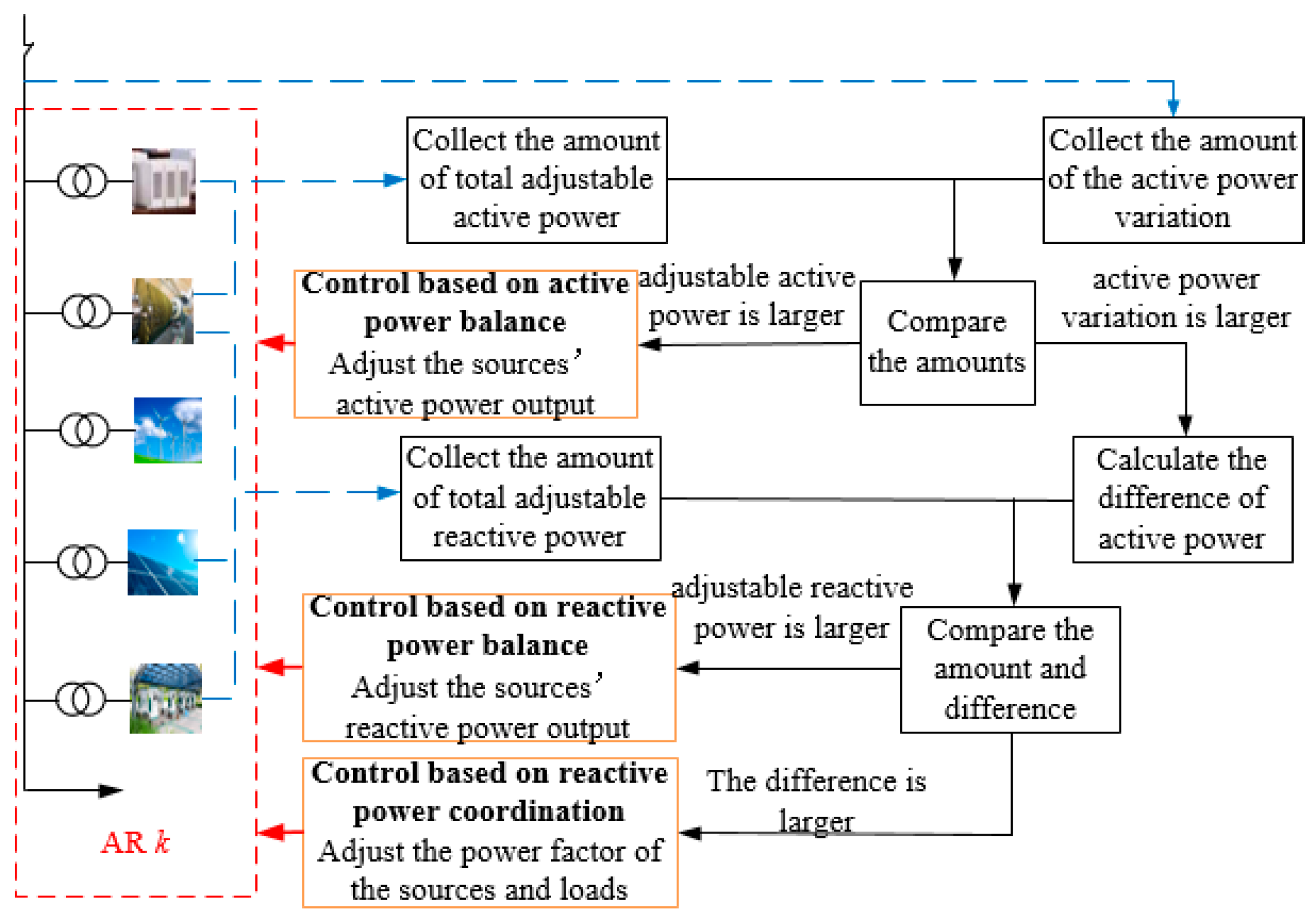
Renewable energy output and EV charging and discharging are random. This characteristic causes large fluctuations on the voltage of ADN, which in turn exceeds the limit of the bus voltage. When the number of sources and loads increase and are adjusted, problems such as real-time response difficulty, large active power loss, and complicated communication system occur. Therefore, dividing the ADN into several ARs containing CSAL is an effective solution. 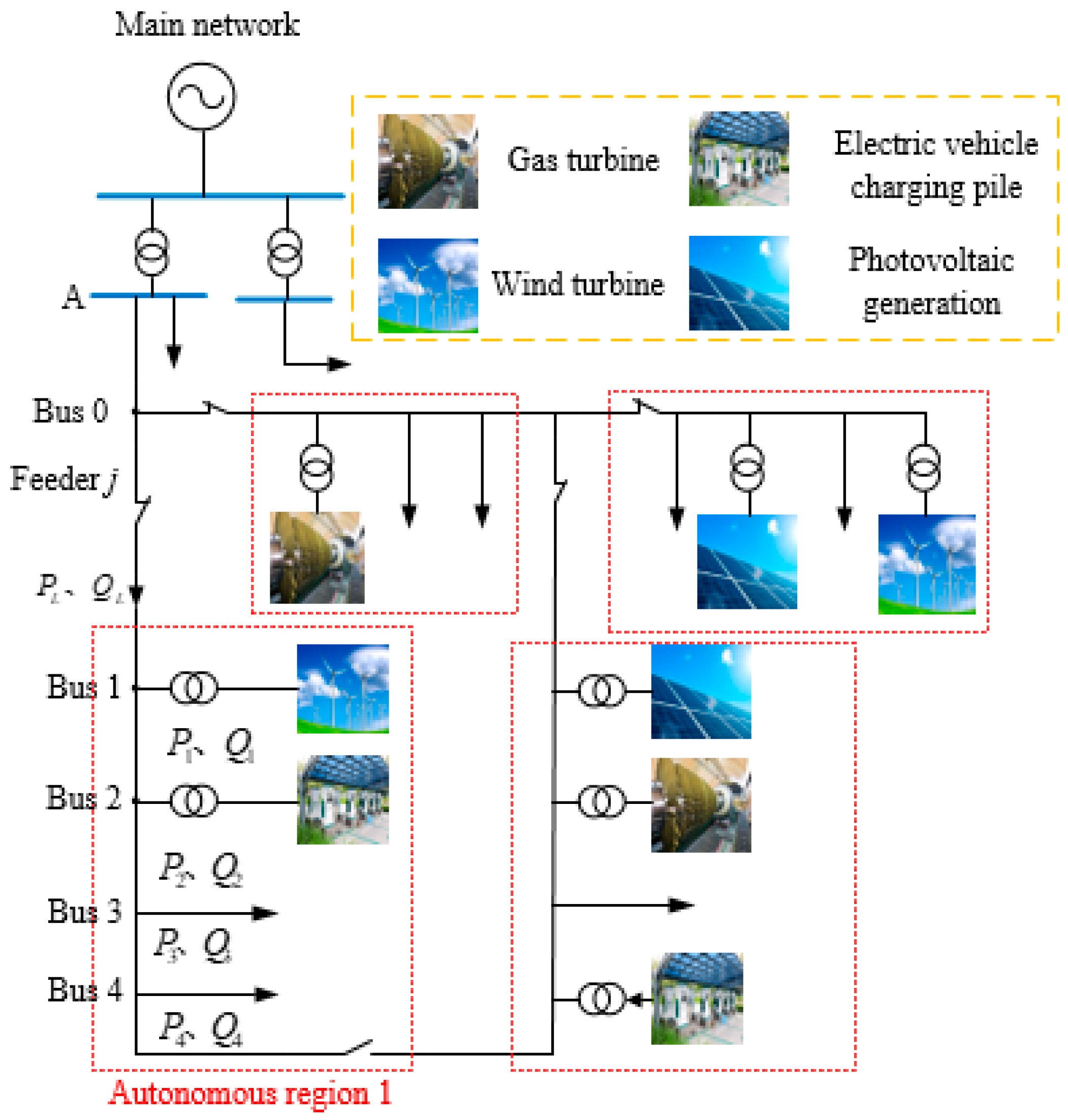The power is independently balanced in each AR to achieve rapid adjustment under power variation [15]. In consideration of the characteristics of ADN, the AR can be divided in accordance with the following principles (Figure 3):

Principle 1: If a controllable source exists between the two circuit breakers on the feeder, this part of ADN can be divided into one AR.

Principle 2: If a controllable source exists between the circuit breakers and the end of the line, this part of ADN can be divided into one AR.

The idea of voltage control through AR is shown in Figure 3. The controllable sources in the AR include active- and reactive-power-adjustable DGs, such as gas and wind turbines, PVs, and energy storages. The controllable loads are mainly EVs. Gas turbines usually do not run as a reactive source; hence, their reactive power output is generally not adjustable. The wind turbines and PVs adopt maximum power tracking control. When the wind speed or sunshine is constant, the output power cannot be increased. However, the active power output can be reduced by abandoning wind or light. When the active output of the wind turbines or PVs is less than their own capacity, the reactive power output can be adjusted and the adjustable reactive capacity is determined by their capacity and active power output. The energy storage output can be adjusted within its limits. The power of the EV is dependent on the capacity of the charging station, and if necessary, the EV can provide feedback to the grid. Therefore, the adjustable active power in any AR $k$ at time $t$ is the sum of the adjustable active power of the gas turbines and energy storages.

$$P_{\mathrm{ak},\mathrm{t}}=P_{\mathrm{agk},\mathrm{t}}+P_{\mathrm{aek},\mathrm{t}}$$

(7)

$$\{\begin{array}{l}{P}_{\mathrm{agk},\mathrm{t}}={\displaystyle \sum _{j_{\mathrm{g}}=1}^{m_{gk}}\left(S_{\mathrm{gk}}^{j_{\mathrm{g}}}-P_{\mathrm{gk},\mathrm{t}}^{j_{\mathrm{g}}}\right)}\\ P_{\mathrm{aek},\mathrm{t}}={\displaystyle \sum _{j_{\mathrm{e}}=1}^{m_{ek}}\left(\sqrt{{\left(S_{\mathrm{ek}}^{j_{\mathrm{e}}}\right)}^2-{\left(Q_{\mathrm{ek},\mathrm{t}}^{j_{\mathrm{e}}}\right)}^2}-P_{\mathrm{ek},\mathrm{t}}^{j_{\mathrm{e}}}\right)}\end{array}$$

(8)

where $P_{ak,t}$, $P_{agk,t}$, and $P_{aek,t}$ are respectively the total adjustable active power, total adjustable active power of gas turbines, and total adjustable active power of energy storages in AR $k$ at time $t$; $S_{gk}^{j_g}$ and $P_{gk,t}^{j_g}$ are respectively the capacity and active power output of the $j_g\mathrm{th}$ gas turbine in AR $k$ at time $t$; and $m_{gk}$ and $m_{ek}$ are respectively the amount of gas turbines and energy storages in AR $k$.

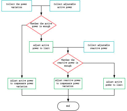
If active power variation occurs in AR $k$ at time $t$ and the active power fluctuation $\Delta P_{k,t}$ is smaller than the adjustable active power in the AR (i.e., $\Delta P_{\mathrm{k},\mathrm{t}}\le P_{\mathrm{ak},\mathrm{t}}$), then the active power in the AR can be adjusted to compensate for the active power variation and the voltage can be controlled. Compared with reactive power adjustment, this method can maximize the economic advantages of distributed generation. At this point, a voltage control method based on active power balance (AP-VC) is adopted to compensate for the active variation in the region by adjusting the active power output of the gas turbines and energy storages. Therefore, the total amount of active and reactive power to be adjusted in region $k$ at time $t+1$ is

$$\{\begin{array}{l}\Delta P_{\mathrm{tk},\mathrm{t}+1}=\Delta P_{\mathrm{k},\mathrm{t}}\\ \Delta Q_{\mathrm{tk},\mathrm{t}+1}=0\end{array}$$

(9)

where $\Delta P_{tk,t+1}$ and $\Delta Q_{tk,t+1}$ are respectively the total active power and reactive power adjustment amount in AR $k$ at time $t$.

If the active power variation amount $\Delta P_{k,t}$ is larger than the adjustable active power in the AR, even if the active power output of the gas turbines and energy storages in the AR are adjusted to their limit, the active power variation cannot be fully compensated. At this point, a difference $P_{ck,t}$ between the active power variation and the adjustable amount remains. The total adjustable reactive power in AR $k$ and its VEAP is

$$\{\begin{array}{l}{Q}_{ak,t}=Q_{awk,t}+Q_{apk,t}+Q_{aek,t}+Q_{avk,t}\\ P_{dak,t}=\frac{X_{1k}}{R_{1k}}{Q}_{ak,t}\end{array}$$

(10)

$$\{\begin{array}{l}{Q}_{\mathrm{awk},\mathrm{t}}={\displaystyle \sum _{j_{\mathrm{w}}=1}^{m_{wk}}\left(\sqrt{{\left(S_{\mathrm{wk}}^{j_{\mathrm{w}}}\right)}^2-{\left(P_{\mathrm{wk},\mathrm{t}}^{j_{\mathrm{w}}}\right)}^2}-Q_{\mathrm{wk},\mathrm{t}}^{j_{\mathrm{w}}}\right)}\\ Q_{\mathrm{apk},\mathrm{t}}={\displaystyle \sum _{j_{\mathrm{p}}=1}^{m_{pk}}\left(\sqrt{{\left(S_{\mathrm{pk}}^{j_{\mathrm{p}}}\right)}^2-{\left(P_{\mathrm{pk},\mathrm{t}}^{j_{\mathrm{p}}}\right)}^2}-Q_{\mathrm{pk},\mathrm{t}}^{j_{\mathrm{p}}}\right)}\\ Q_{\mathrm{aek},\mathrm{t}}={\displaystyle \sum _{j_{\mathrm{e}}=1}^{m_{ek}}\left(\sqrt{{\left(S_{\mathrm{ek}}^{j_{\mathrm{e}}}\right)}^2-{\left(P_{\mathrm{ek},\mathrm{t}}^{j_{\mathrm{e}}}\right)}^2}-Q_{\mathrm{ek},\mathrm{t}}^{j_{\mathrm{e}}}\right)}\\ Q_{\mathrm{avk},\mathrm{t}}={\displaystyle \sum _{j_{\mathrm{v}}=1}^{m_{vk}}\left(\sqrt{{\left(S_{\mathrm{vk}}^{j_{\mathrm{v}}}\right)}^2-{\left(P_{\mathrm{vk},\mathrm{t}}^{j_{\mathrm{v}}}\right)}^2}-Q_{\mathrm{vk},\mathrm{t}}^{j_{\mathrm{v}}}\right)}\end{array}$$

(11)

where $Q_{ak,t}$ and $P_{dak,t}$ are respectively the total amount of adjustable reactive power and VEAP of AR $k$ at time $t$; $R_{1k}$ and $X_{1k}$ are respectively the resistance and reactance of the line connecting the AR $k$ to the former net; $Q_{awk,t}$, $Q_{apk,t}$, $Q_{aek,t}$ and $Q_{avk,t}$ are respectively the total adjustable amount of reactive power through the wind turbines, PVs, energy storages, and EVs in AR $k$ at time $t$; $S_{wk}^{j_w}$, $S_{pk}^{j_g}$, and $S_{vk}^{j_v}$ are the capacity of the $j_w\mathrm{th}$ wind turbines, $j_p\mathrm{th}$ PVs, and $j_v\mathrm{th}$ EVs, respectively, in AR $k$; $P_{wk,t}^{j_w}$, $P_{pk,t}^{j_g}$, and $P_{vk,t}^{j_v}$ are the active power output of the $j_w\mathrm{th}$ wind turbines, $j_p\mathrm{th}$ PVs, and $j_v\mathrm{th}$ EVs, respectively in AR $k$ at time $t$; and $m_{wk}$, $m_{pk}$, and $m_{vk}$ are respectively the amount of wind turbines, PVs, and EVs in AR $k$.

If $P_{ck,t}$ is less than the VEAP of AR $k$ at this point, a voltage control method based on reactive power balance (RP-VC) is adopted. After the gas turbines and energy storages in the AR have been adjusted to the limit, the reactive output of the wind turbines, PVs, energy storages, and EVs is adjusted to compensate for the active power variation in the AR to stabilize the voltage. Therefore, the total amount of active and reactive power to be adjusted in AR $k$ at time $t+1$ is

$$\{\begin{array}{l}\Delta P_{\mathrm{tk},\mathrm{t}+1}=P_{\mathrm{ak},\mathrm{t}}\\ \Delta Q_{\mathrm{tk},\mathrm{t}+1}=\frac{P_{\mathrm{ck},\mathrm{t}}{R}_{1k}}{X_{1k}}\end{array}$$

(12)

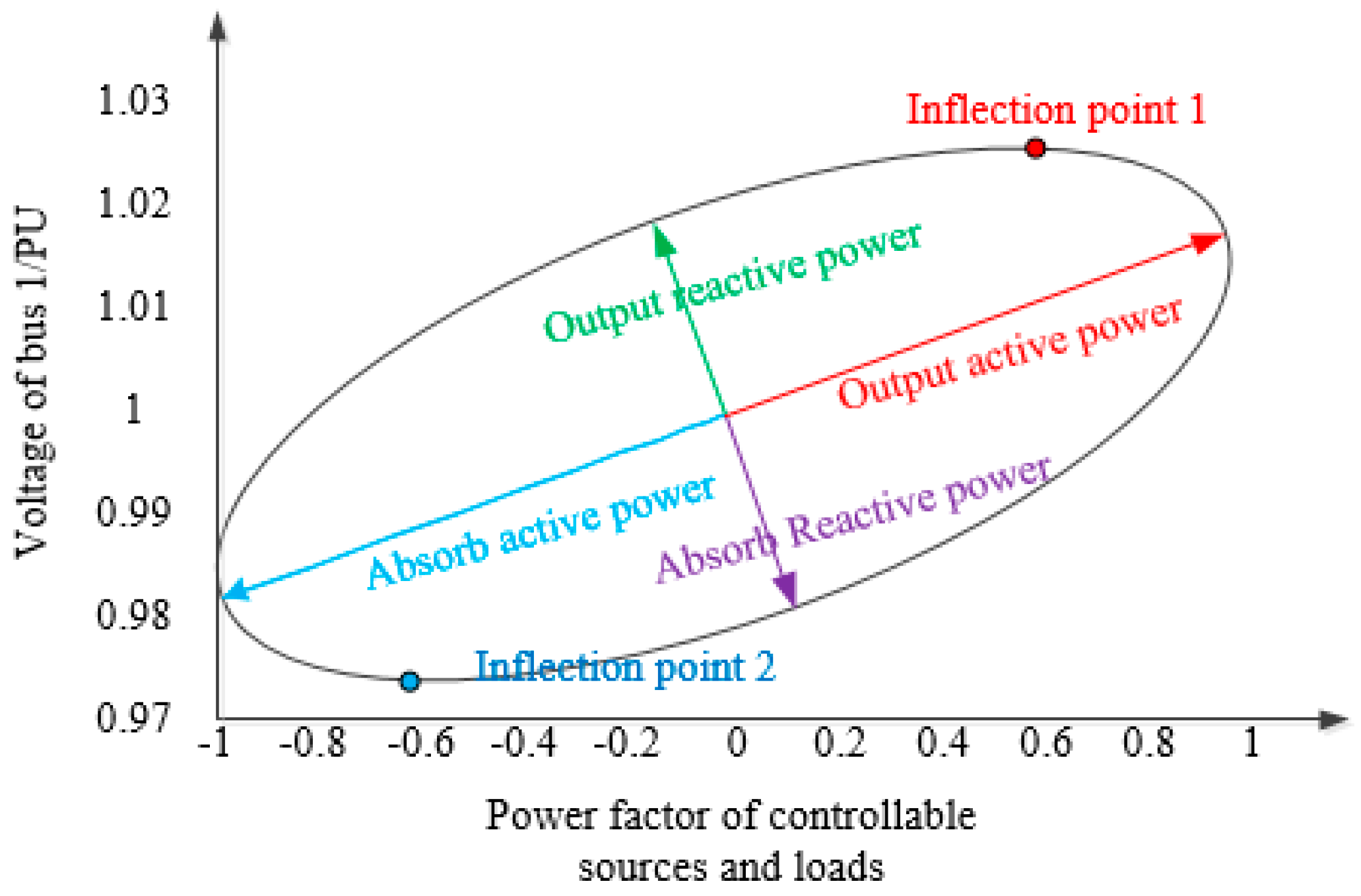
If the active power variation is larger than the sum of the VEAP and adjustable active power of AR $k$, then $\Delta P_{\mathrm{k},\mathrm{t}}>P_{\mathrm{ak},\mathrm{t}}+P_{\mathrm{dak},\mathrm{t}}$. Although the active and reactive power outputs of all controllable sources and loads in the AR have been adjusted to their limit values, the active power variation of the AR cannot be fully compensated. At this point, all controllable sources and loads in the area operates at a rated capacity and the power factor of wind turbines, PVs, energy storages, and EVs must be adjusted to compensate for active power variation. When all the sources and loads in AR $k$ run at the inflection point, the sum of the total active power and EVAP reaches its limit $P_{ak,t}^{\max }$.

$$P_{ak,t}^{\max }=P_{\mathrm{agk},\mathrm{t}}+{\displaystyle \sum _{i=1}^n\Delta P_{ik,t}+}{\displaystyle \sum _{i=1}^n\frac{X_{1k}}{R_{1k}}\Delta Q_{ik,t}}$$

(13)

$$\{\begin{array}{l}\Delta P_{\mathrm{ik},\mathrm{t}}={\omega }_{Gk}{\mathrm{S}}_{ik}-P_{ik,t}\\ \Delta Q_{\mathrm{ik},\mathrm{t}}=\sqrt{1-{\omega }_{Gk}^2}{\mathrm{S}}_{ik}-Q_{ik,t}\end{array}$$

(14)

where $n$ is the sum of $m_{ek}$, $m_{wk}$, $m_{pk}$, and $m_{pk}$; $\Delta P_{ik,t}$ and $\Delta Q_{ik,t}$ are respectively the adjustable active and reactive power amounts of the controllable source or load connected to bus $i$ in AR $k$ at time $t$; ${\omega }_{Gk}$ is the power factor of the inflection point of AR $k$; and $P_{ik,t}$ and $Q_{ik,t}$ are respectively the active and reactive power outputs of the controllable source or load connected to bus $i$ in AR $k$ at time $t$.

If $\Delta P_{k,t}$ is less than the limit, that is, $\Delta P_{\mathrm{k},\mathrm{t}}\le P_{ak,t}^{\max }$, the voltage control method based on active and reactive power coordination (ARP-VC) is adopted. First, the gas turbines and energy storages in the AR are adjusted to the limit. Second, the power factor of the wind turbines, PVs, energy storages, and EVs is adjusted in accordance with the active power deficiency to compensate for the active power variation in the AR and to stabilize the voltage. Finally, the total amount of active and reactive power to be adjusted in region $k$ at time $t+1$ is

$$\Delta P_{\mathrm{tk},\mathrm{t}+1}+\frac{X_{1k}}{R_{1k}}\Delta Q_{\mathrm{tk},\mathrm{t}+1}=\Delta P_{\mathrm{k},\mathrm{t}}$$

(15)

If $\Delta P_{\mathrm{k},\mathrm{t}}>P_{ak,t}^{\max }$, then the active power fluctuation cannot be completely compensated by adjusting the power in the AR. In this case, the voltage should be regulated using a transformer or something similar.

To realize the voltage control method, the information of power change and adjustable active and reactive power in the AR is necessary. Therefore, the power metering infrastructure should be installed on the line between the first bus of each AR and its former bus to get the power change and on the DGs to get the adjustable active and reactive power. The information needs to be transmitted to a central processing unit by the information and communication technology (ICT) to calculate the amount of adjustment of the DG power and then to transmit it back to the DGs to complete the voltage control.

4. Voltage Control Model Based on the Power Coordination of the AR

4.1. Active Power Optimization Model of the AR

When $\Delta P_{\mathrm{k},\mathrm{t}}\le P_{\mathrm{ak},\mathrm{t}}$, the active power adjustment involves the gas turbines and energy storages. The cost should be prioritized at this point because the active power variation is not large. The amount of total active power adjustment is optimally distributed among the gas turbines and energy storages. The objective function is as follows:

$$F_1=\min \left\{{\displaystyle \sum _{j_g=1}^{m_{gk}}\left[a_{j_g}{\left(P_{gk,t}^{j_g}\right)}^2+b_{j_g}{P}_{gk,t}^{j_g}+c_{j_g}\right]+{\displaystyle \sum _{j_e=1}^{m_{ek}}{\alpha }_{j_e}{P}_{ek,t}^{j_e}}}\right\}$$

(16)

$$\Delta P_{\mathrm{k},\mathrm{t}}={\displaystyle \sum _{j_g=1}^{m_{gk}}\Delta P_{gk,t+1}^{j_g}}+{\displaystyle \sum _{e=1}^{m_{ek}}\Delta P_{ek,t+1}^{j_e}}$$

(17)

$$P_{\mathrm{gk},\min }^{j_g}\le P_{gk,t+1}^{j_g}\le P_{\mathrm{gk}.\max }^{j_g}$$

(18)

$$P_{ek,\min }^{j_e}\le P_{ek,t+1}^{j_e}\le P_{ek,max}^{j_e}$$

(19)

$$\{\begin{array}{c}{P}_{gk,t+1}^{j_g}-P_{gk,t}^{j_g}\le U_{\mathrm{k}.\mathrm{t}}{R}_{\mathrm{u},{\mathrm{j}}_g}+\left(1-U_{\mathrm{k}.\mathrm{t}}\right)P_{gk,max}^{j_g}\\ P_{gk,t}^{j_g}-P_{gk,t+1}^{j_g}\le U_{\mathrm{k}.\mathrm{t}+1}{R}_{\mathrm{d},{\mathrm{j}}_g}+\left(1-U_{\mathrm{k}.\mathrm{t}+1}\right)P_{gk,max}^{j_g}\end{array}$$

(20)

where $a_{j_g}, b_{j_g}, c_{j_g}$ are the energy consumption parameter of the $j_g\mathrm{th}$ gas turbine; ${\alpha }_{j_e}$ is the active power output parameter of the $j_e\mathrm{th}$ energy storage; $\Delta P_{gk,t+1}^{j_g}$ and $\Delta P_{ek,t+1}^{j_e}$ are respectively the active power adjustment amount of the $j_g\mathrm{th}$ gas turbine and $j_e\mathrm{th}$ energy storage in AR k at time $t+1$; $P_{gk,max}^{j_g}$ and $P_{gk,min}^{j_g}$ are respectively the maximum and minimum output of the $j_g\mathrm{th}$ gas turbine in AR $k$; $P_{ek,min}^{j_e}$ and $P_{ek,max}^{j_e}$ are respectively the minimum and maximum outputs of the $j_e\mathrm{th}$ energy storage in AR $k$; and $R_{u, j_g}$ and $R_{d, j_g}$ are respectively the ramp up and ramp down rates of the $j_g\mathrm{th}$ gas turbine.

The constraint of Equation (17) ensures that the amount of active power adjustment is equal to the variation. The constraints of Equations (18) and (19) are the limits of the active power output of the gas turbines and energy storages. The constraint of Equation (20) is the change rate limit of the active power output.

4.2. Reactive Power Optimization Model of the AR

When $\Delta P_{k,t}> P_{ak,t}$ and $\Delta P_{ck,t} \le P_{dak,t}$, the active power of the AR fluctuates considerably. Even if the gas turbines and the energy storages reach the limit output, the active fluctuation cannot be compensated. Therefore, the adjustable reactive power in the AR must compensate for the active fluctuation. Given that the reactive power cost is almost negligible, the obvious active power fluctuates will lead to considerable fluctuations in voltage. The voltage control method proposed in this study can maintain the voltage of the first bus in each AR. Thus, targeting the lowest deviation of other bus voltages in each region from the first bus is effective. Then, the total reactive power in the AR is adjusted using wind power, PV, energy storages, and EVs. The objective function is as follows:

$$F_2=\min \left[{\displaystyle \sum _{i=1}^{n_k}{\left(V_{ki}-V_{Nk}\right)}^2}\right]$$

(21)

$${\displaystyle \sum _{j_w=1}^{m_{wk}}\Delta Q_{\mathrm{wk},\mathrm{t}+1}^{j_w}+{\displaystyle \sum _{j_p=1}^{m_{pk}}\Delta Q_{\mathrm{pk},\mathrm{t}+1}^{j_p}+{\displaystyle \sum _{j_e=1}^{m_{ek}}\Delta Q_{\mathrm{ek},\mathrm{t}+1}^{j_e}}}}+{\displaystyle \sum _{j_v=1}^{m_{vk}}\Delta Q_{\mathrm{vk},\mathrm{t}+1}^{j_v}}=\frac{\left(\Delta P_{k,t}-P_{ak,t}\right)R_{1k}}{X_{1k}}$$

(22)

$$P_{gk,t+1}^{j_g}=P_{\mathrm{gk}.\max }^{j_g}$$

(23)

$$\{\begin{array}{l}{\left(Q_{wk,t+1}^{jw}\right)}^2+{\left(P_{wk,t+1}^{jw}\right)}^2\le {\left(S_{wk}^{jw}\right)}^2\\ {\left(Q_{pk,t+1}^{jp}\right)}^2+{\left(P_{pk,t+1}^{jp}\right)}^2\le {\left(S_{pk}^{jp}\right)}^2\\ {\left(Q_{ek,t+1}^{je}\right)}^2+{\left(P_{ek,t+1}^{je}\right)}^2\le {\left(S_{ek}^{je}\right)}^2\\ {\left(Q_{vk,t+1}^{jv}\right)}^2+{\left(P_{vk,t+1}^{jv}\right)}^2\le {\left(S_{vk}^{jv}\right)}^2\end{array}$$

(24)

where $V_{ik}$ and $V_{Nk}$ are the voltages of $i\mathrm{th}$ bus and first bus, respectively, in AR $k$; $n_k$ is the number of buses in AR $k$; and $\Delta Q_{wk,t+1}^{j_w}$, $\Delta Q_{pk,t+1}^{j_p}$, $\Delta Q_{ek,t+1}^{j_e}$, and $\Delta Q_{vk,t+1}^{j_v}$ are the reactive power adjustment amounts of the $j_w\mathrm{th}$ wind turbine, $j_p\mathrm{th}$ PV, $j_e\mathrm{th}$ energy storage, and $j_v\mathrm{th}$ EV, respectively, in AR $k$ at time $t+1$.

The constraints of Equations (22) and (23) reflect the control method based on RP-VC. The constraint of Equation (24) restricts the power output of sources and loads that participated in the adjustment.

4.3. Active and Reactive Power Cooperation Optimization Model of the AR

If $\Delta P_{\mathrm{k},\mathrm{t}}>P_{\mathrm{ak},\mathrm{t}}+P_{\mathrm{dak},\mathrm{t}}$ and $\Delta P_{\mathrm{k},\mathrm{t}}\le P_{ak,t}^{\max }$, then the active power variation in the AR is large and the active and reactive power outputs of all the power supplies in the region cannot be compensated for the active power variation. Thus, the active and reactive power of the CSAL must be coordinated. Given the large variation of active power, the degree of bus voltage deviation is evident. An excessive discarding of wind and light is not conducive to economic operation. A reduction in EV charge quantity also affects the normal power consumption of users. Therefore, the degree of bus voltage deviation and the discard amount of wind, light, and EV charging are optimized at this stage. The objective function is as follows:

$$F_3=\min \left[{\displaystyle \sum _{i=1}^{n_k}{\left(V_{ki}-V_{Nk}\right)}^2}+{\beta }_w{P}_{wk,t+1}+{\beta }_p{P}_{pk,t+1}+{\beta }_v{P}_{vk,t+1}\right]$$

(25)

$${\displaystyle \sum _{i=1}^n\left(\frac{\Delta Q_{ik,t+1}{X}_{1k}}{R_{1k}}+\Delta P_{ik,t+1}\right)}=\Delta P_{k,t}$$

(26)

$$\{\begin{array}{l}{P}_{wk,t+1}^{jw}\le P_{wk,t+1, max}^{jw}\\ P_{pk,t+1}^{jp}\le P_{pk,t+1, max}^{jp}\\ \frac{SO{C}_{k,T_{end}}^{jv}-SO{C}_{k,t+1}^{jv}}{T_{end}-\left(t+1\right)}\le P_{vk,t+1}^{jv}\le P_{vk,t+1, max}^{jv}\end{array}$$

(27)

$$\{\begin{array}{l}{\left(Q_{wk,t+1}^{jw}\right)}^2+{\left(P_{wk,t+1}^{jw}\right)}^2={\left(S_{wk}^{jw}\right)}^2\\ {\left(Q_{pk,t+1}^{jp}\right)}^2+{\left(P_{pk,t+1}^{jp}\right)}^2={\left(S_{pk}^{jp}\right)}^2\\ {\left(Q_{ek,t+1}^{je}\right)}^2+{\left(P_{ek,t+1}^{je}\right)}^2={\left(S_{ek}^{je}\right)}^2\end{array}$$

(28)

$$\{\begin{array}{l}{P}_{wk,t+1}^{jw}\ge S_{wk}^{jw}{\omega }_{Gk}\\ P_{pk,t+1}^{jp}\ge S_{pk}^{jp}{\omega }_{Gk}\end{array}$$

(29)

where $P_{wk,t+1}$, $P_{pk,t+1}$, and $P_{vk,t+1}$ are the loss amounts of the total active power of wind turbines, PVs, and EVs, respectively, in AR $k$ at time $t+1$; ${\beta }_w$, ${\beta }_p$, and ${\beta }_v$ are respectively the unit values of the active power that wind turbine, PV, and EV loses; $P_{wk,t+1,max}^{j_w}$, $P_{pk,t+1,max}^{j_p}$, and $P_{vk,t+1,max}^{j_v}$ are respectively the active power output upper limit of $j_w\mathrm{th}$ wind turbines, $j_p\mathrm{th}$ PVs, and j_vth EVs in AR $k$ at time $t+1$; $SO{C}_{k,T_{end}}^{jv}$ is the charge status of the $j_v\mathrm{th}$ EVs in AR $k$ at time $T_{end}$; $T_{end}$ is the charging end time of the $j_v\mathrm{th}$ EVs in AR $k$, which can be notified in advance by the users to the charging station; and $SO{C}_{k,t+1}^{jv}$ is the charge status of the $j_v\mathrm{th}$ EVs in AR $k$ at time $t+1$.

The constraint of Equation (26) shows the power coordination based on the ARP-VC control method. The constraint of Equation (27) is the active power limit of the wind turbines, PVs, and EVs, and this ensure that the EVs can join the voltage control and has no influence on the users. The constraint of Equation (28) ensures that the wind turbines, PVs, energy storages, and EVs work at rated capacity. The constraint of Equation (29) ensures that the wind turbines and PVs work in a low active power-abandoned status.

4.4. Solver of the Optimization Model

The particle swarm optimization (PSO) algorithm is widely used due to its simplicity, easy implementation, strong global search ability, and fast calculation speed. The PSO is optimized in s-dimensional space and initialized N random particles. All particles have a fitness determined by the objective function. The zth particle contains a position vector $x_z=\left[x_{z1},x_{z2},\cdots ,x_{zs}\right]$ and a speed vector $v_z=\left[v_{z1},v_{z2},\cdots ,v_{zs}\right]$. In each iteration, the ith particle updates itself by two “extreme values”. One is the optimal solution $p{b}_z=\left[p{b}_{z1},p{b}_{z2},\cdots ,p{b}_{zs}\right]$, which is found by the ith particle in the iterative process, and the other is the optimal solution $gb=\left[g{b}_1,g{b}_2,\cdots ,g{b}_s\right]$, which is found by all particles in the iterative process.

$$\{\begin{array}{l}{v}_{ik}^{t+1}=\omega v_{ik}^t+c_{1}ran{d}_1\left(p{b}_{ik}^t-x_{ik}^t\right)+c_{2}ran{d}_2\left(g{b}_k^t-x_{ik}^t\right)\\ x_{ik}^{t+1}=x_{ik}^t+v_{ik}^{t+1}\end{array}$$

(30)

where $v_{zs}^t$ and $x_{zs}^t$ are the s-dimensional speed and value of the zth particle when tth iteration; $p{b}_{zs}^t$ is the best s-dimensional value of the zth particle after $t$ iterations; $g{b}_s^t$ is the best s-dimensional value of all the particles after $t$ iterations; $v_{zs}^{t+1}$ and $x_{zs}^{t+1}$ are the s-dimensional speed and value of the zth particle when $t+1\mathrm{th}$ iteration; $\rho$ is the inertia of speed; $c_1,c_2$ are the study factors; and $ran{d}_1,ran{d}_2$ are random numbers between 0 and 1.

The flow of the PSO is shown in the Figure 4. The position vector of each particle is one of the solutions of the optimization. In this paper, the position vector of the particles is composed by the active power and reactive power of the DGs which participate in the power compensation; the value of each dimension of the particles’ position vector corresponds to the active power or reactive power output of the DG. The particle fitness corresponds to the function value of the three optimization models ($F_1,F_2,F_3$). The smaller the function value is, the better the fitness of the particle is. Before the PSO iterations, at first, set the end condition of the iteration, the amount, the inertia, and the study factor of the particles during the PSO operation. Then, initialize each particle; the initial position of the particle is a random combination of the DGs’ output power. During the iterations, first calculate the fitness of each particle by the objective function. Then, update the population optimal solution and the individual optimal solution. After this, update the velocity vector and the position vector according to Equation (30). Loop this process until the end condition is satisfied; the optimal fitness of all particles and its corresponding output of the DGs are the results of the PSO.

5. Case Study

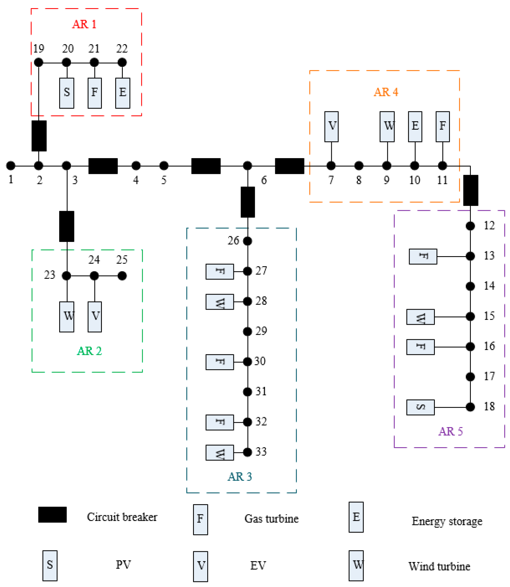
IEEE (Institute of Electrical and Electronics Engineers)-33 study system is a standard distribution network system and its line impedance parameters, load power, and structure are equivalent to the actual distribution network. The IEEE-33 study system has been widely used in the research study of distribution network. Therefore, the system is used to verify the control method proposed in this paper. In this study, DG and EVs are added to the IEEE-33 system to verify the effectiveness of the above methods, as shown in Figure 5. A balanced bus 1 is connected to the main grid. The allowable operating range of the bus voltage is 0.95–1.05 PU. The initial power of system load, voltage of swing bus, etc. are the original values of the system. In the case of increasing power consumption, light intensity and wind speed from 7:00 a.m. to 10:00 a.m. are simulated. In the control of the voltage in the distribution network, the time interval is usually several minutes [11], so this paper chooses to control the power output of the sources every 20 min. The environment to perform the optimization is specifically as follow: The computer processor is Intel core i5, RAM is 8 GB, and MATLAB/MATPOWER perform the optimization used. The time of each optimization is about 2 s.

Table 1. IEEE-33 bus system gas turbine parameters.

Unit	Upper Limit of Active Power (KW)	Lower Limit of Active Power (KW)	a	b	c
13	180	54	200	100	0
16	210	63	150	150	0
27	160	48	75	200	0
30	200	60	200	100	0
32	220	66	150	150	0

is the parameters of the gas turbines. When the gas turbines are put into voltage control, their active power must between the upper limit and the lower limit. The parameters a, b, and c are the generation costs when they generate. The values of a, b, and c are from the cost optimization parameters in MATPOWER.

In accordance with the division principle of the AR, the sample system can be divided into five ARs. The first bus of AR 3 is bus 26, and the first bus of the AR 5 is bus 12. Buses 15, 28, and 33 are connected to wind turbines with capacities of 340, 330, and 340 KVA, respectively. Bus 18 is connected to the PV with a capacity of 320 KVA, and buses 13, 16, 27, 30, and 32 are connected with gas turbines. 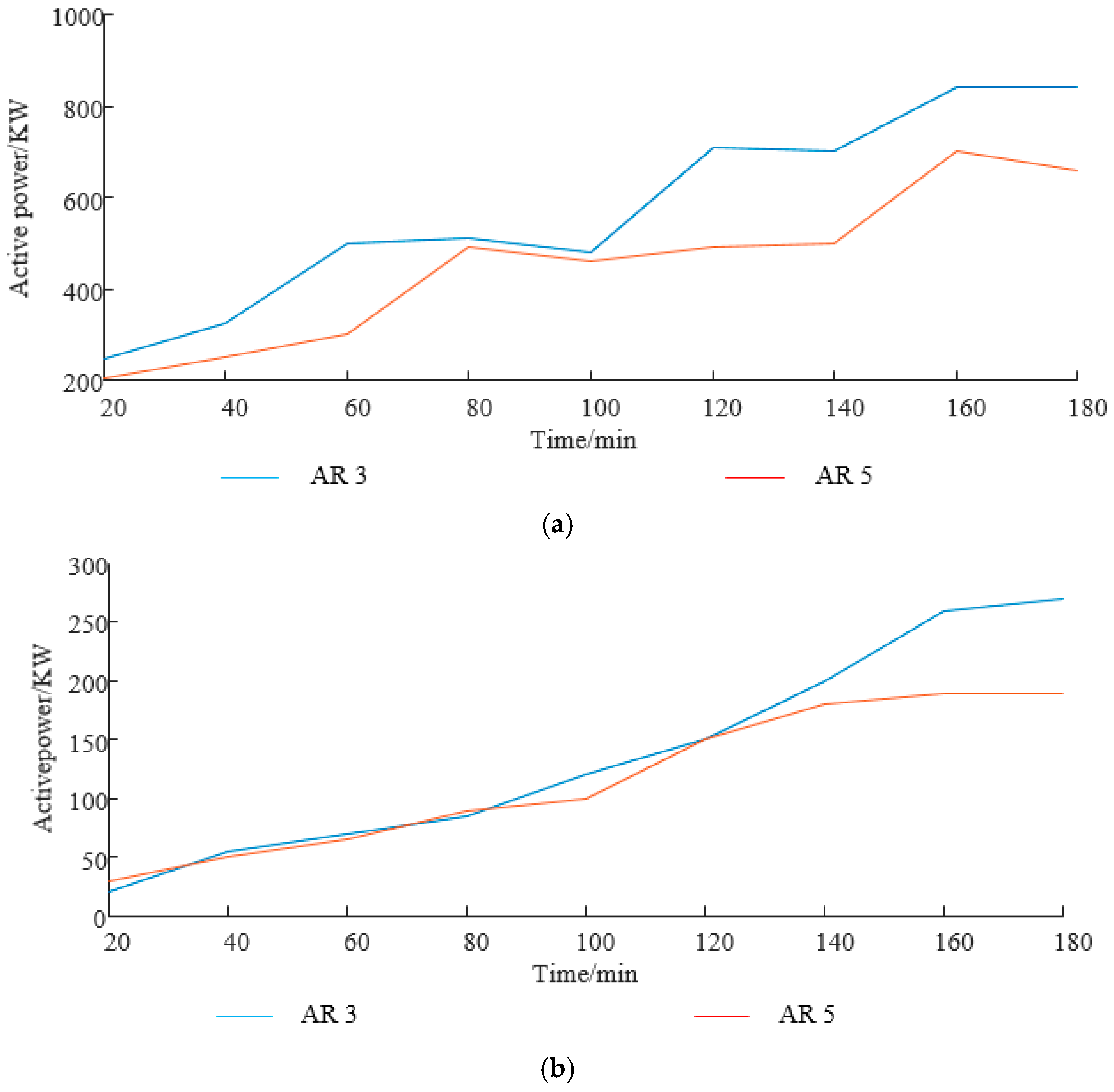The gas turbines’ active power output limits and cost factor are shown in Table 1. All the initial active power outputs of gas turbines are 100 KW, and the reactive power outputs is 0 KVar. The initial active power output of wind turbines and PVs is 200 KW, and the reactive power output is 0 KVar. Assuming that the active power of the loads is connected to buses 12, 14, 17, 26, 29, and 31 in ARs 3 and 5, the wind turbines and PVs connected to buses 15, 18, 28, and 33 change. Among them, the wind turbines of buses 28 and 33 reach the upper limits of 160 and 180 min, respectively. Figure 6 is the total fluctuation amounts of the loads, wind turbines, and PV in ARs 3 and 5 at 20–180 min. The voltage fluctuations of the buses are shown in

Table 2. Bus voltage fluctuations in ARs 3 and 5.

Bus	Time/Min
	0	20	40	60	80	100	120	140	160	180
12	0.9639	0.9476	0.9449	0.9397	0.9268	0.9311	0.9294	0.9319	0.9145	0.9181
13	0.9624	0.9464	0.9435	0.9380	0.9249	0.9298	0.9283	0.9309	0.9128	0.9169
14	0.9618	0.9458	0.9428	0.9373	0.9240	0.9291	0.9277	0.9304	0.9120	0.9162
15	0.9618	0.9461	0.9431	0.9375	0.9243	0.9296	0.9283	0.9311	0.9127	0.9170
16	0.9616	0.9461	0.9430	0.9373	0.9241	0.9296	0.9284	0.9312	0.9126	0.9172
17	0.9610	0.9458	0.9425	0.9368	0.9236	0.9293	0.9283	0.9311	0.9124	0.9173
18	0.9604	0.9453	0.9421	0.9364	0.9232	0.9289	0.9281	0.9309	0.9122	0.9171
26	0.9615	0.9488	0.9464	0.9386	0.9361	0.9399	0.9310	0.9337	0.9248	0.9264
27	0.9607	0.9477	0.9451	0.9373	0.9349	0.9387	0.9299	0.9327	0.9235	0.9252
28	0.9571	0.9425	0.9396	0.9317	0.9294	0.9338	0.9250	0.9281	0.9181	0.9200
29	0.9542	0.9385	0.9353	0.9271	0.9250	0.9296	0.9207	0.9239	0.9133	0.9153
30	0.9533	0.9370	0.9336	0.9255	0.9233	0.9281	0.9192	0.9225	0.9119	0.9140
31	0.9519	0.9344	0.9309	0.9227	0.9206	0.9255	0.9167	0.9202	0.9097	0.9119
32	0.9516	0.9342	0.9307	0.9225	0.9204	0.9254	0.9165	0.9201	0.9096	0.9118
33	0.9516	0.9341	0.9307	0.9225	0.9204	0.9254	0.9167	0.9203	0.9098	0.9121

. Without control, the voltage drops rapidly and falls outside the safe operating voltage range.

According to the control method proposed in this study, the total active power variation is smaller than the adjustable active power capacity in AR 3 at 0–40 min. Therefore, the voltage control method based on active balance is adopted to control the active power output of the gas turbines and thus to suppress the fluctuation of the voltage. The optimization variables are the active power output of gas turbines 27, 30, and 32 during this period. Thereafter, the loads and the output of wind turbines and PVs continue to change; thus, the active power variation is greater than the adjustable active power. After 40 min, avoiding voltage overshoot becomes impossible by only adjusting active power. At 40–160 min, the adjustable reactive power in the ARs is greater than the difference and the voltage fluctuation can be suppressed by reactive power adjustment. At this point, the voltage control method based on reactive power balance is used to control the reactive power output of wind turbines and PVs to compensate for active power variation. The optimization variables are the reactive power output of wind turbines 28 and 33 during this period. At 160–180 min, the active power variation is too large even if the reactive power output of all the wind turbines and PVs are adjusted to their limits; thus, the effect of active power change cannot be fully compensated. At this point, a voltage control method based on active and reactive power coordination is needed. The power factor of the controllable sources in AR 3 is adjusted, and the total active and reactive power output in the AR are coordinated to compensate for the active power variation and to reduce the voltage fluctuation. The optimization variables are the active power and reactive power outputs of wind turbines 28 and 33 during this period. Similarly, for AR 5, the AP-VC and RP-VC methods are adopted at 0–60 and 60–180 min, and the optimization variables are the active power output of gas turbines 13 and 16 and reactive power output of wind turbines 15 and PV 33, respectively.

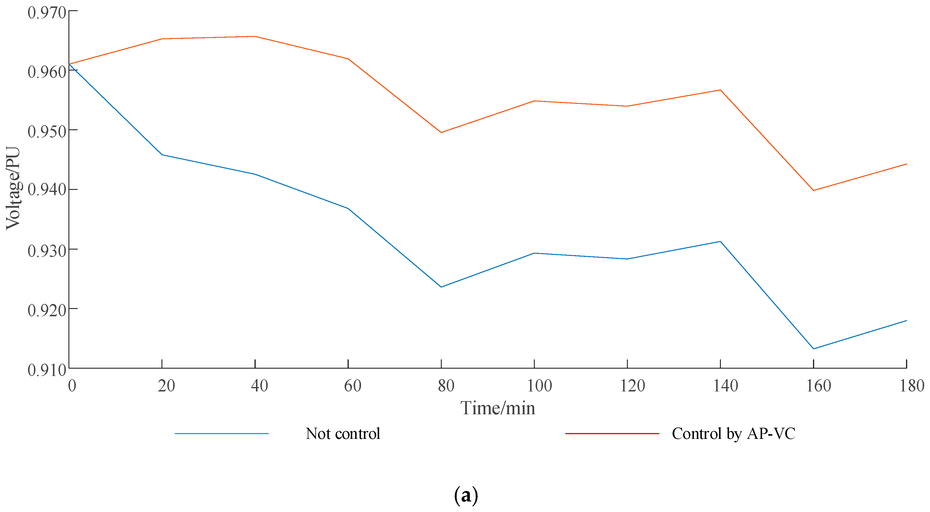
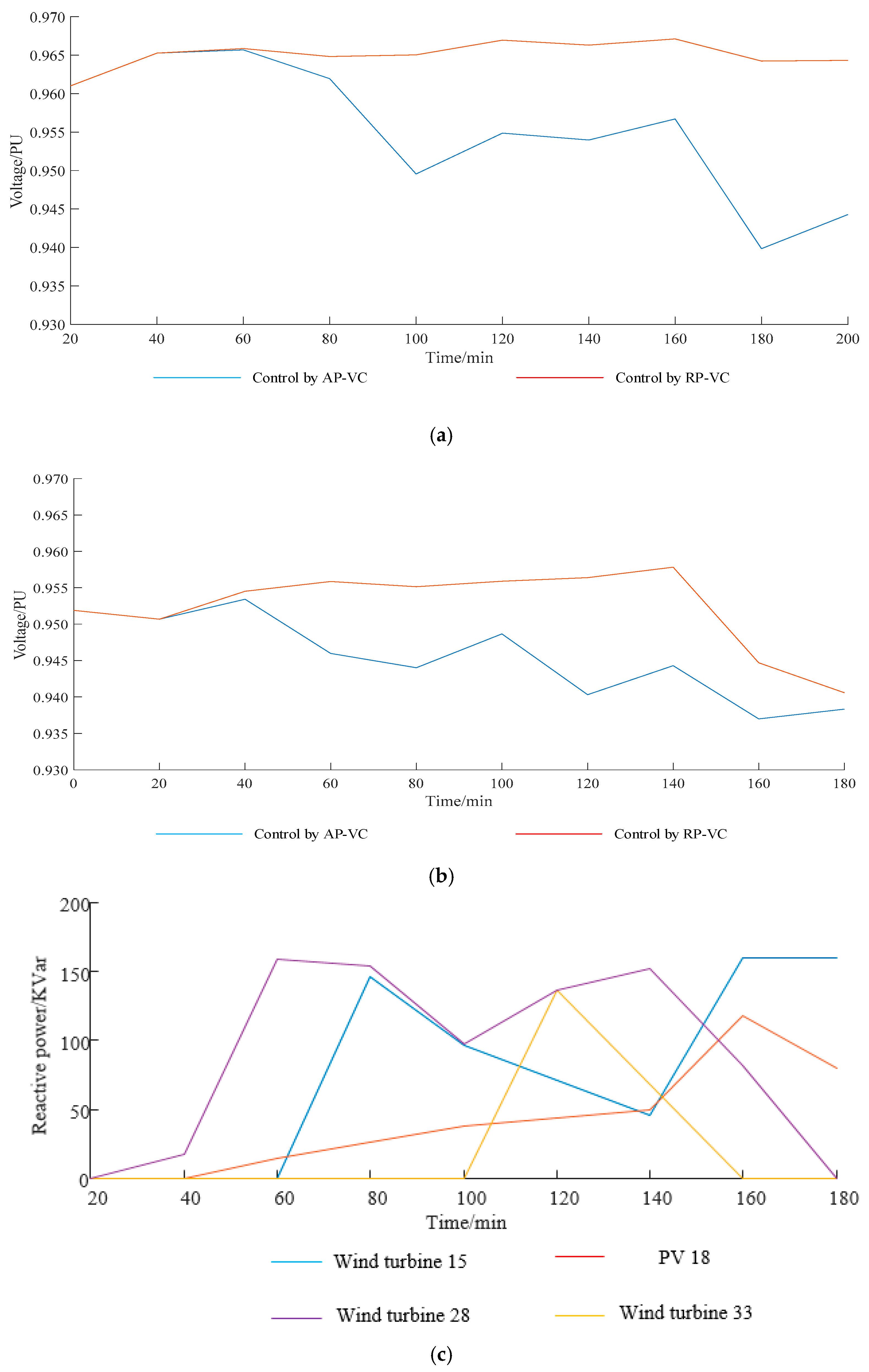
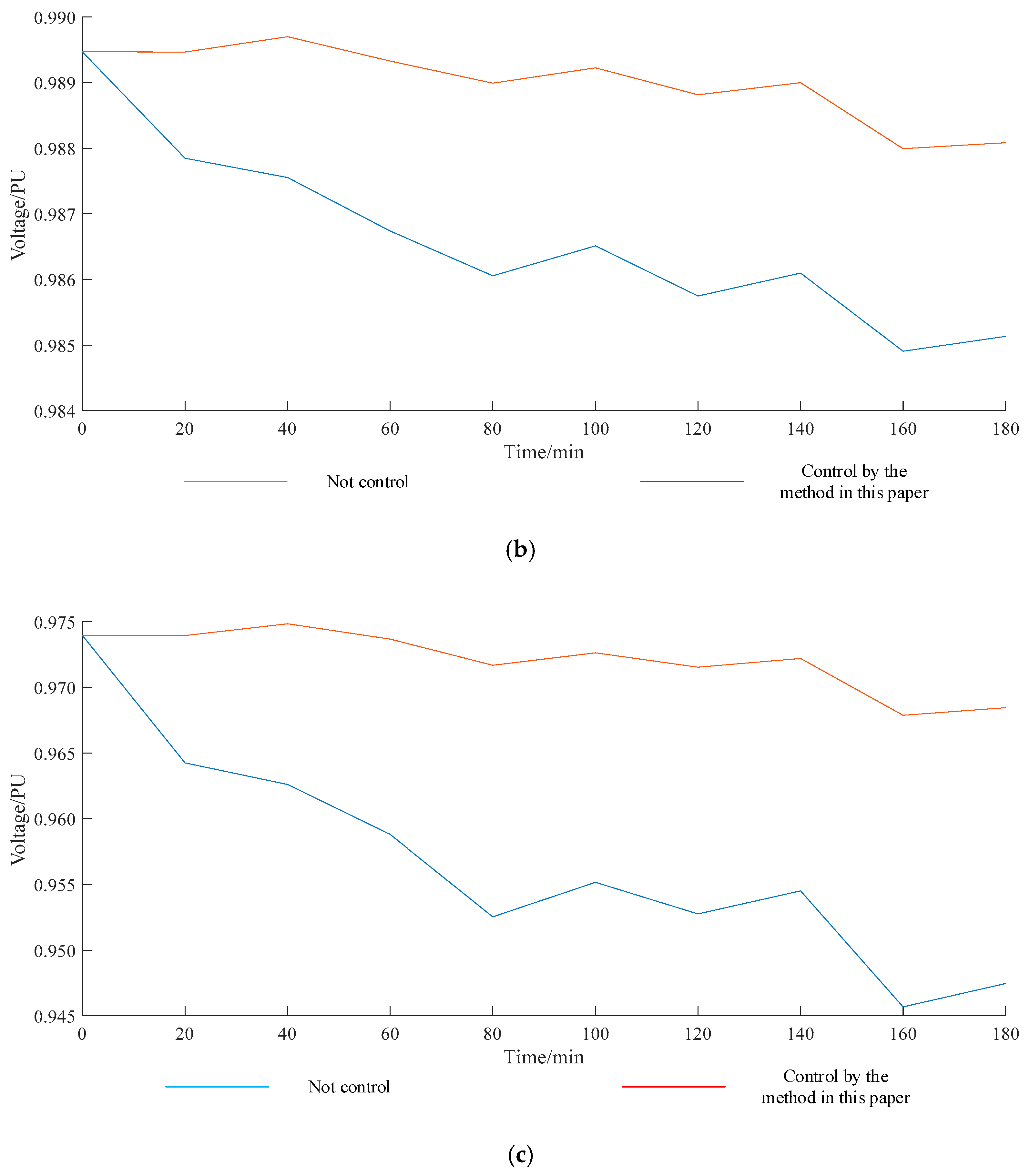
Figure 7a,b show the voltages of buses 17 and 31 when not controlled or under AP-VC control. The two buses are not connected to DG directly and are near the end of the line; hence, active power variation considerably affects the two buses. Under the variation of active power, the blue line is the fluctuation of the bus voltage when not controlled and the red line is the fluctuation of the bus voltage when the active power output is controlled by the AP-VC. Figure 7c shows the corresponding amount of adjustment in the active power output of the gas turbines. The gas turbines of ARs 3 and 5 have active power outputs reaching upper limits of 40 and 60 min, respectively. Compared with an uncontrolled scenario, adjusting the active power output of the gas turbines can remarkably reduce the drop in voltage amplitude. After the active power output of the gas turbines reaches the maximum, the drop in voltage amplitude in bus 17 is reduced by 0.0285 PU and that in bus 31 is reduced by 0.0274 PU. At 0–40 min, the active power margin is enough to compensate for the active power variation and the voltage fluctuation of bus 17 is small. Given that the gas turbines’ active power output reaches the upper limit after 60 min, the bus voltage begins to drop with the active power variation. With a 140 KW load connected to bus 12 at 80 min, the voltage of bus 17 drops sharply and exceeds the limit, falling to 0.9487 PU. Similarly, after 40 min, the voltage of bus 31 begins to drop due to lack of active power support; thus, its voltage drops to 0.9460 PU at 60 min. The minimum voltages for the two buses are 0.9426 and 0.9390 PU. At 40 min, the output of gas turbine 13 in AR 5 is 220 KW and the output of gas turbine 16 is 180 KW; hence, the power generation unit cost is 14.59. If the active output is equally distributed to two gas turbines, then each output is 200 KW and the unit cost of power generation is 16.06; thus, the voltage of bus 17 is 0.0006 lower than AP-VC. When the active fluctuation is not large, the active power distribution affects the bus voltage slightly but considerably influences the cost. After the active cost has been optimized, the power generation cost is reduced by 9.15%.

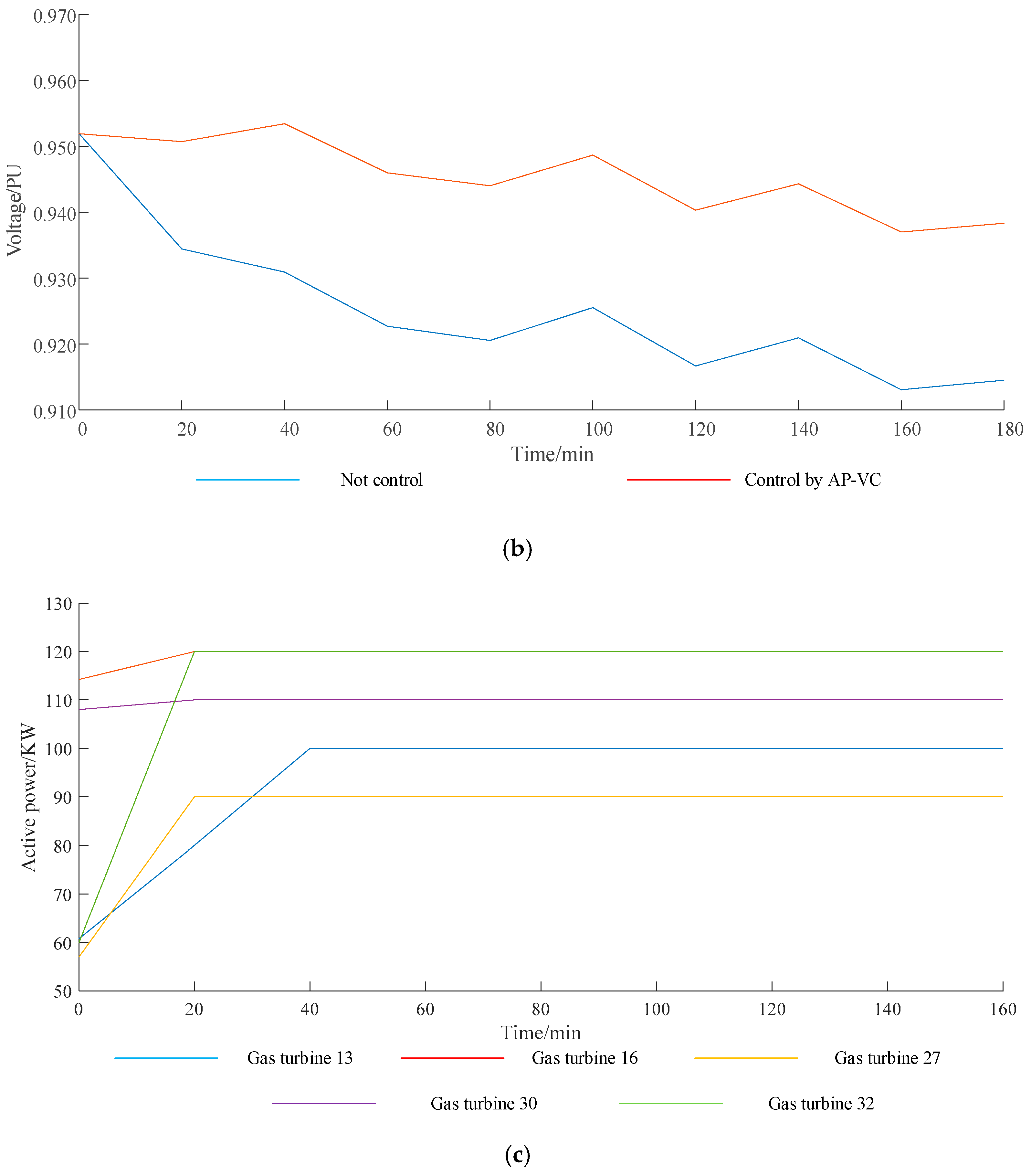
The bus voltages controlled by RP-VC and AP-VC or only by AP-VC are shown in Figure 8a,b. RP-VC is used to control the reactive power of the wind turbines and PVs in ARs 5 and 3 after 60 and 40 min, respectively. Figure 8c shows the reactive power output of the wind turbines and PVs at various times. Given the insufficient reactive power of AR 5, the voltage of bus 17 remains above 0.96 PU after 60 min and the voltage fluctuation is small. Similarly, before 140 min, the voltage of bus 31 is stable above 0.95 PU; however, after 160 min, the reactive margin is greatly reduced because the active power output of the wind turbines of AR 3 is close to the rated value and generating sufficient reactive power to support voltage is impossible; thus, the voltage of bus 31 significantly drops from 0.9553 PU to 0.9404 PU.

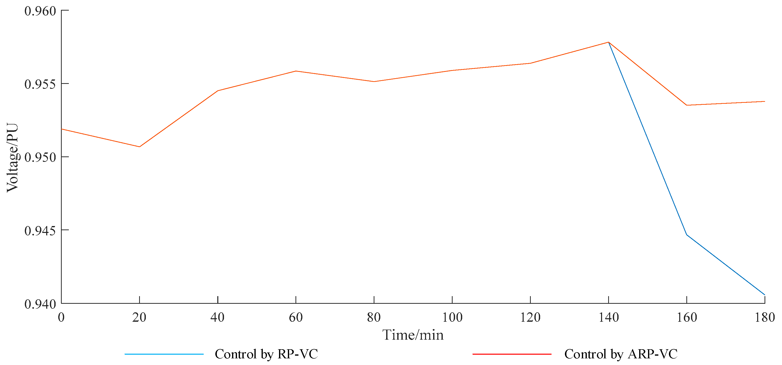
After 160 min, the voltage of bus 31 controlled by ARP-VC is shown in Figure 9. Controlled by the ARP-VC method, the wind turbines discard a small amount of wind energy, thereby obtaining a large amount of reactive power to compensate for active power change. Compared with the control method that does not adopt the ARP-VC, the voltage of bus 31 does not drop sharply at 160–180 min and is stable above 0.95PU when adopt it. The cost of abandoning wind and light in this study is based on the parameters in Reference [24], which are all converted to 0.267 (KW·20 min). The total amount of abandoned wind in AR 5 is optimized to 86 and 101 kW at 160 and 180 min, respectively. The costs of abandoned wind in the next 20 min are 22.962 and 26.967, respectively. At 160 min, the sum of the voltage deviations of all buses in AR 3 is 56.647, whereas that of all the buses in AR 3 is 54.263 at 180 min.

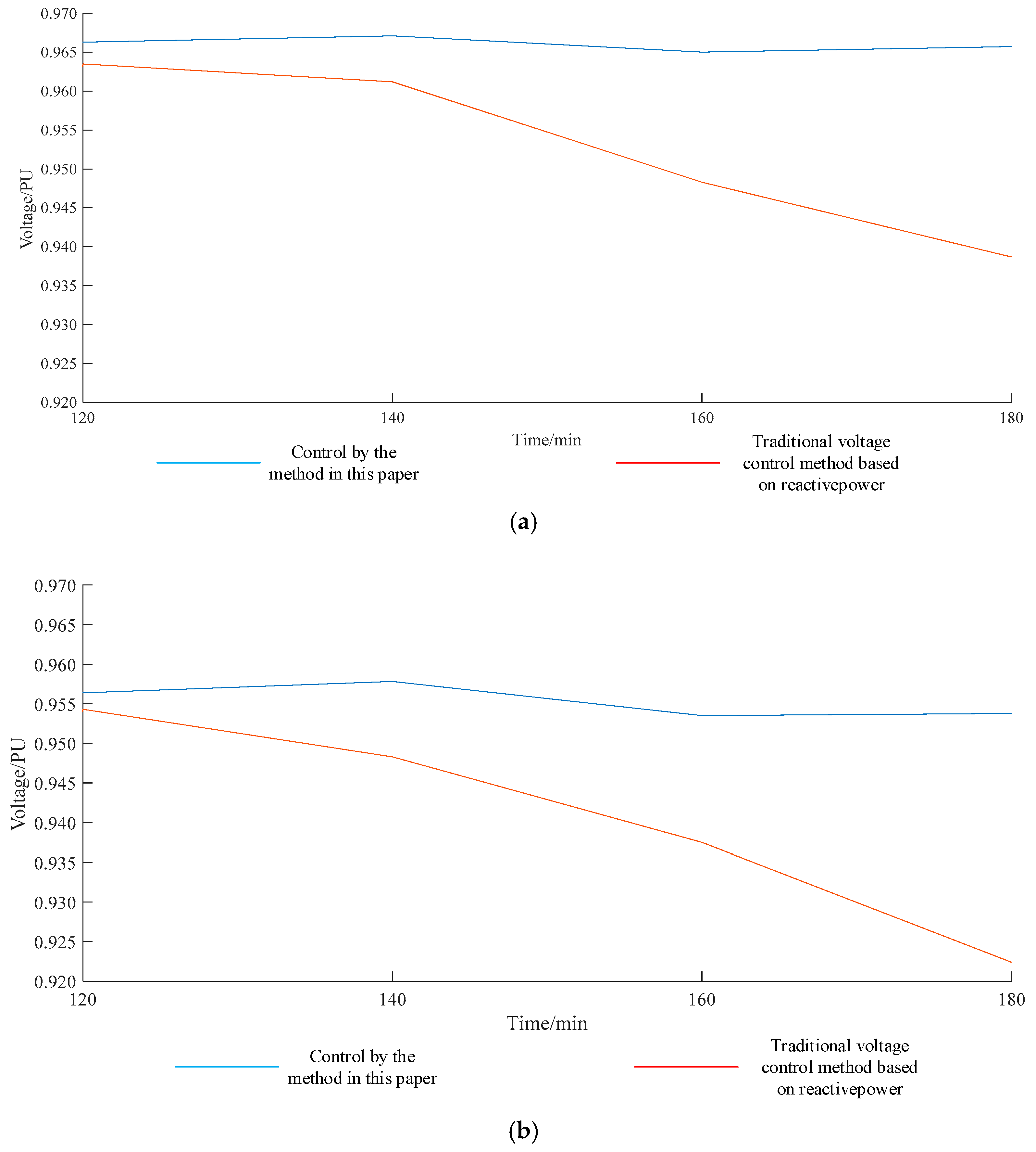
When only the traditional reactive power control method is used to control the voltage, only the reactive power output of wind turbines and PVs can be used because ARs 3 and 5 do not have an independent reactive power compensation device. In AR 3 at 120 min, the active power demand increases by 560 kW whereas the VEAP of the wind turbines and PVs can only reach 431 KW. In AR 5 at 160 min, the active demand increases by 510 KW whereas the VEAP can only reach 307 KW. Moreover, the growth rate of the loads’ active power demand is greater than the output of the wind turbines and PVs; the increase in their active power output remarkably decreases their reactive power margin. Therefore, after 120 min, the reactive power cannot compensate for the active power variation, causing the bus voltage to drop rapidly, as shown in Figure 10.

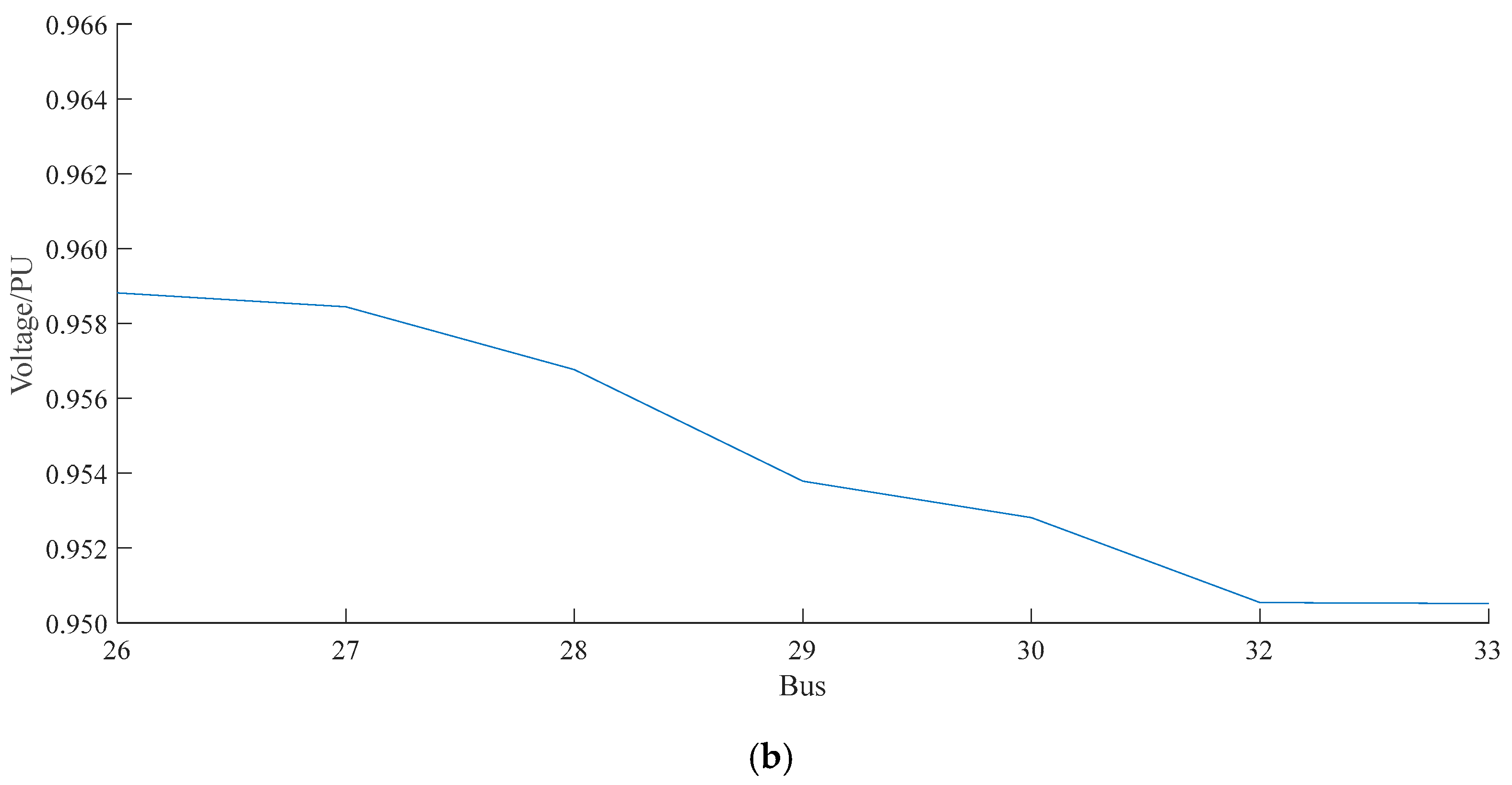
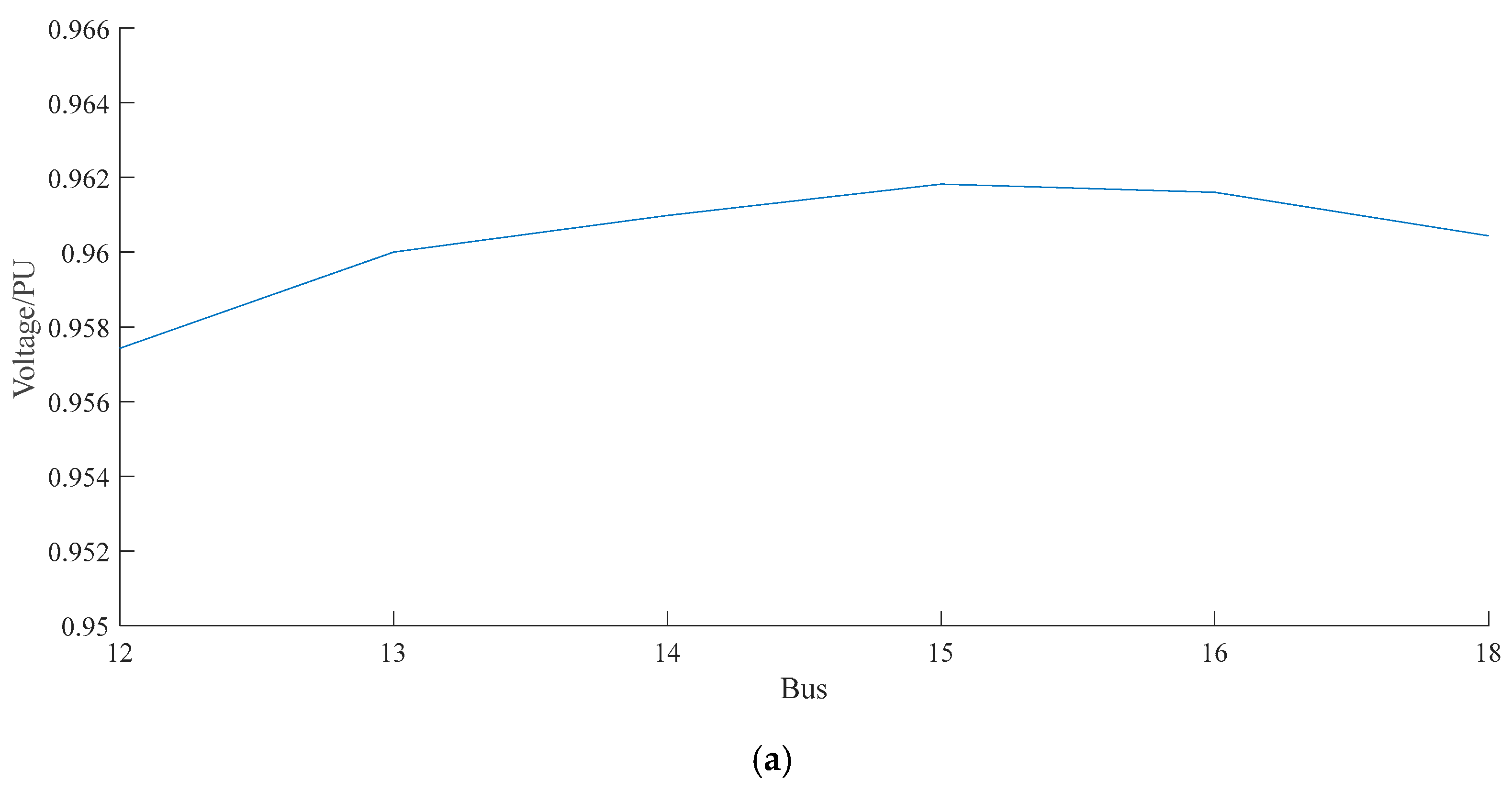
Figure 11 shows the minimum voltage of all buses in ARs 3 and 5 except buses 17 and 31 during the period of 20–180 min. Through active voltage control, the voltage of all buses is restored at 0.95 PU or more.

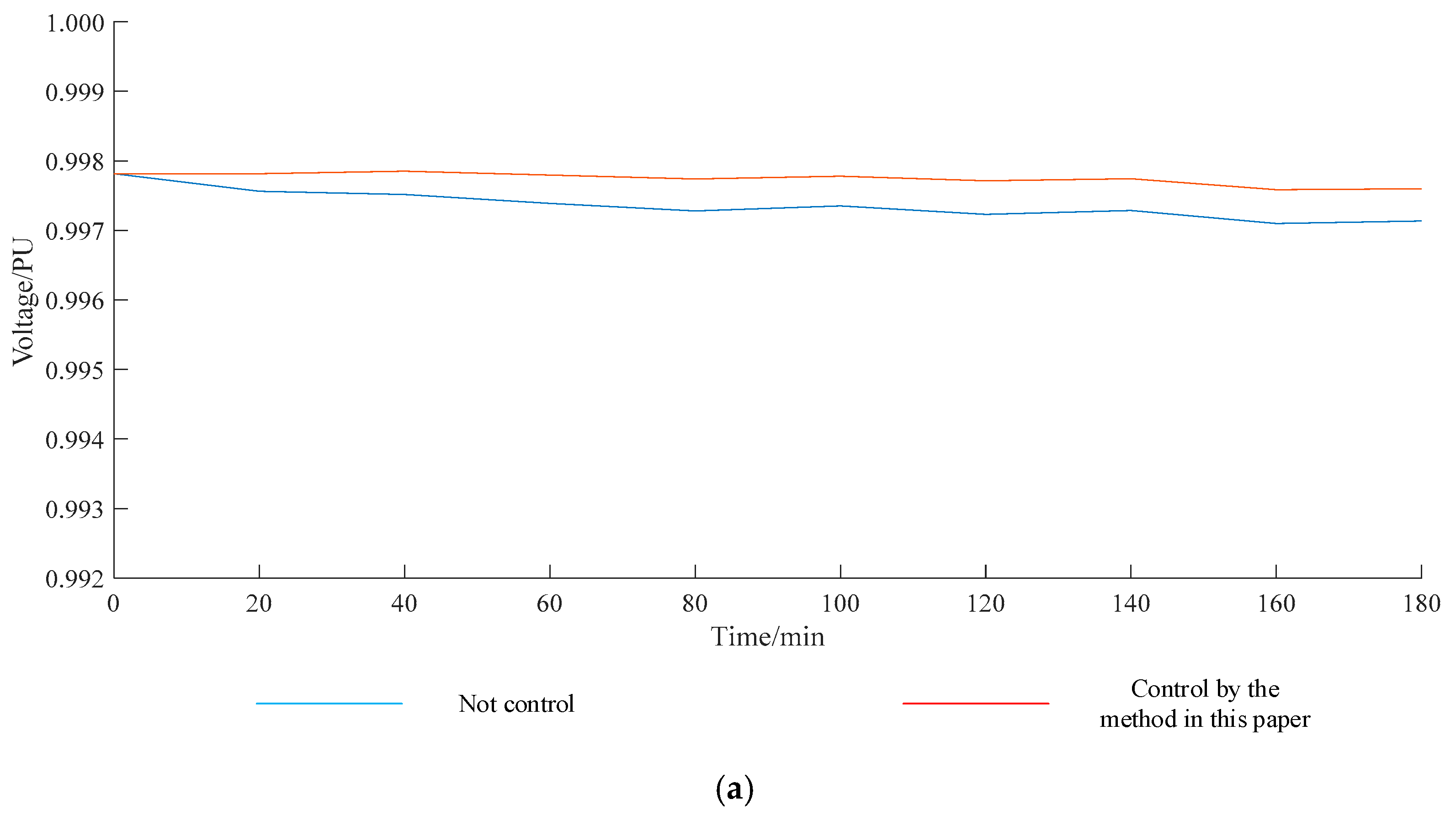
Figure 12 shows the lowest bus voltages in ARs 1, 2, and 4 before and after control. Although active power variation occurs in ARs 3 and 5, the bus voltage in the other three ARs are affected in varying degrees. The bus voltage of AR 4, which is directly connected to AR 5, is mostly affected by variation and falls below 0.95 PU after 160 min if not controlled. Adjusting the power of ARs 3 and 5 stabilizes the bus voltage in the other three ARs. The minimum voltage of AR 4 is restored to 0.97 PU.

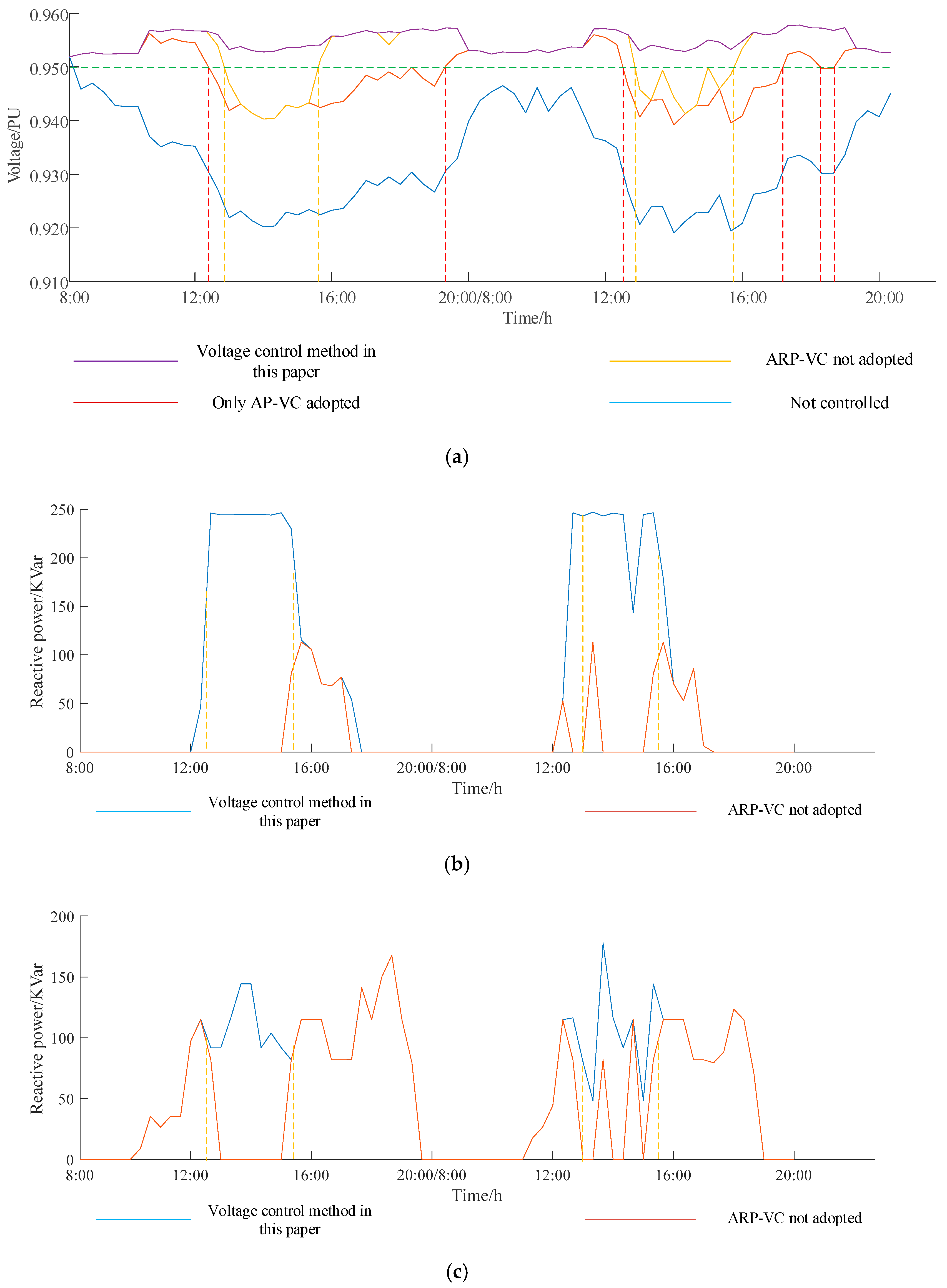
To verify that time has no effect on the method in this paper, the control effects of AR 3 from 8 am to 8 pm in two days is shown in Figure 13. As the active power of loads and wind turbines changes, the voltage of bus 31 fluctuates greatly if not controlled and it drops under the lower limit for a long time; the lowest voltage is 0.9191. If controlled by the method in this paper and if the active power is fully compensated, the voltage is above 0.95PU and very stable. The lowest voltage is 0.9512 and the highest voltage is 0.9578. If ARP-VC is not adopted, the voltage is under 0.95PU from 12:40 to 15:40 during the first day and from 13:00 to 15:40 during the second day. This is due to the high active power output of wind turbines, which causes the wind power to fail to generate enough reactive power to support the voltage, as shown in Figure 13b,c. If only the gas turbines are put into the voltage control, the voltage is under the lower limit from 12:20 to 19:20 during the first day and from 12:20 to 16:40 during the second day.

6. Conclusions

To solve the voltage fluctuation caused by active power variation in ADNs, this study proposes a voltage control method based on active and reactive power coordination. First, the active power variation in each AR is independently adjusted by dividing the ADN into several ARs. Second, the active and reactive power margins and the upper limit of adjustable power in each AR are calculated. In accordance with the degree of variation, different controls are adopted for compensation. The PSO algorithm is used to adjust the power of DGs to suppress voltage fluctuation. The main contribution in this paper is the voltage control by coordinating the active and reactive power output of the sources. The case study has shown that, controlled by the method in this paper, the voltage can keep steady under a huge variation in the power, which may cause the voltage to drop under the lower limit even if all the sources work at the maximum output status but do not coordinate their active and reactive power.

In the power control process of DGs, there may be situations where it is necessary to reduce the active power output of DGs to obtain more reactive power outputs to support voltage. Reducing the active power output of the DGs will affect the profit of its owner. At this time, the DSO needs to compensate the owner by purchasing auxiliary services, etc., and to reduce the loss of the owner to let them actively respond to the power control.

References

1. Li, Y.; Tian, X.S.; Liu, C. Study on voltage control in distribution network with renewable energy integration. In Proceedings of the 2017 IEEE Conference on Energy Internet and Energy System Integration, Beijing, China, 4 January 2018. [Google Scholar]
2. Li, R.; Wang, W.; Xia, M.C. Cooperative Planning of Active Distribution System with Renewable Energy Sources and Energy Storage Systems. IEEE Access 2018, 6, 5916–5926. [Google Scholar] [CrossRef]
3. Thomson, M.; David, G. Infield Network Power-Flow Analysis for a High Penetration of Distributed Generation. IEEE Trans. Power Syst. 2007, 22, 1157–1162. [Google Scholar] [CrossRef]
4. Chen, C.S.; Lin, C.H.; Hsieh, W.L. Enhancement of PV Penetration with DSTATCOM in Taipower Distribution System. IEEE Trans. Power Syst. 2013, 28, 1560–1567. [Google Scholar] [CrossRef]
5. Marcincin, O.; Medvec, Z. Active charging stations for electric cars. In Proceedings of the 2015 16th International Scientific Conference on Electric Power Engineering (EPE), Kouty nad Desnou, Czech Republic, 20 July 2015. [Google Scholar]
6. Rautiainen, A.; Repo, S.; Jarventausta, P.; Mutanen, A.; Vuorilehto, K.; Jalkanen, K. Statistical Charging Load Modeling of PHEVs in Electricity Distribution Networks Using National Travel Survey Data. IEEE Trans. Smart Grid 2012, 3, 1650–1659. [Google Scholar] [CrossRef]
7. Lassila, J.; Haakaana, J.; Tikka, V.; Partanen, J. Methodology to Analyze the Economic Effects of Electric Cars as Energy Storages. IEEE Trans. Smart Grid 2012, 3, 506–516. [Google Scholar] [CrossRef]
8. Ruiz-Rodriguez, F.J.; Hernandez, J.c.; Jurado, F. Probabilistic Load-Flow Analysis of Biomass-Fuelled Gas Engines with Electrical Vehicles in Distribution Systems. Energies 2017, 10, 1536. [Google Scholar] [CrossRef]
9. Ruiz-Rodriguez, F.J.; Hernandez, J.C.; Jurado, F. Voltage behavior in radial distribution systems under the uncertainties of photovoltaic systems and electric vehicle. Int. Trans. Electr. Energy Syst. 2018, 28, e2490. [Google Scholar] [CrossRef]
10. Hernandez, J.C.; Sanchez-Sutil, F.; Vidal, P.G.; Rus-Casas, C. Primary frequency control and dynamic grid support for vehicle-to-grid in transmission systems. Int. J. Electr. Power Energy Syst. 2018, 100, 152–166. [Google Scholar] [CrossRef]
11. Hernandez, J.C.; Ruiz-Rodriguez, F.J.; Jurado, F. Modelling and assessment of the combined technical impact of electric vehicles and photovoltaic generation in radial distribution systems. Energy 2017, 141, 316–332. [Google Scholar] [CrossRef]
12. Koutsoukis, N.C.; Siagkas, D.O.; Georgilakis, P.S. Online Reconfiguration of Active Distribution Networks for Maximum Integration of Distributed Generation. IEEE Trans. Autom. Sci. Eng. 2017, 14, 437–448. [Google Scholar] [CrossRef]
13. Wang, Z.Y.; Luo, D.L.; Li, R.Q. Research on the active power coordination control system for wind/photovoltaic/energy storage. In Proceedings of the 2017 IEEE Conference on Energy Internet and Energy System Integration (EI2), Beijing, China, 4 January 2018. [Google Scholar]
14. Berry, I.; Heinzmann, J. Economics of energy storage for dispatchable solar. In Proceedings of the 2016 IEEE Power and Energy Society General Meeting (PESGM), Boston, MA, USA, 17–21 July 2016. [Google Scholar]
15. Yi, Y.; Dong, L.; Qing, Z. Distributed Generation Coordination Control Based on Active Distribution Network on Multiple Time Scales. Autom. Electr. Power Syst. 2014, 38, 192–198+203. [Google Scholar]
16. Byrne, R.H.; Nguyen, T.A.; Copp, D.A. Energy Management and Optimization Methods for Grid Energy Storage Systems. IEEE Access 2017, 6, 13231–13260. [Google Scholar] [CrossRef]
17. Zhou, H.; Zhang, W.; Cong, R. Optimization of reactive power for active distribution network with power electronic transformer. In Proceedings of the 2015 12th International Conference on the European Energy Market (EEM), Lisbon, Portugal, 19–22 May 2015. [Google Scholar]
18. Ding, T.; Liu, S.Y.; Yuan, W. A Two-Stage Robust Reactive Power Optimization Considering Uncertain Wind Power Integration in Active Distribution Networks. IEEE Trans. Sustain. Energy 2016, 7, 301–311. [Google Scholar] [CrossRef]
19. Hincapie, R.A.; Granada, M.; Gallego, R.A. Optimal planning of secondary distribution systems considering distributed generation and network reliability. In Proceedings of the 2016 IEEE ANDESCON, Arequipa, Peru, 2 February 2017. [Google Scholar]
20. Tang, Z.Y.; Hill, D.J.; Liu, T. Fast Distributed Reactive Power Control for Voltage Regulation in Distribution Networks. IEEE Trans. Power Syst. 2019, 34, 802–805. [Google Scholar] [CrossRef]
21. Chen, S.X.; Eddy, Y.S.F.; Gooi, H.B. A Centralized Reactive Power Compensation System for LV Distribution Networks. IEEE Trans. Power Syst. 2015, 30, 274–284. [Google Scholar] [CrossRef]
22. Marra, F.; Yang, G.Y.; Fawzy, Y.T. Improvement of Local Voltage in Feeders with Photovoltaic Using Electric Vehicles. IEEE Trans. Power Syst. 2013, 28, 3515–3516. [Google Scholar] [CrossRef]
23. Zheng, W.Y.; Wu, W.C.; Zhang, B.M. A Fully Distributed Reactive Power Optimization and Control Method for Active Distribution Networks. IEEE Trans. Smart Grid 2016, 7, 1021–1033. [Google Scholar] [CrossRef]
24. Zheng, N.; Ding, X.Q.; Guan, Z.C. Active-reactive coordination optimization of distribution network based on scene method. Power Syst. Technol. 2019, 43, 1640–1651. [Google Scholar]
Figure 1. Schematic diagram of active distribution network (ADN).
Energies 12 04364 g001
Figure 2. Influence of bus 1 generation and load power factors on bus voltage.
Energies 12 04364 g002
Figure 3. Principle of voltage control based on regional power coordination.
Energies 12 04364 g003
Figure 4. Flow of the particle swarm optimization (PSO) algorithm.
Energies 12 04364 g004
Figure 5. IEEE-33 study system.
Energies 12 04364 g005
Figure 6. Amount of active change in autonomous regions (ARs) 3 and 5: (a) Total active power change in the region and (b) total wind power and photovoltaic (PV) active power output change in the region.
Energies 12 04364 g006
Figure 7. Comparison of the control effects: (a) AR 5 bus 17 voltage; (b) AR 3 bus 31 voltage; and (c) gas turbine active power output change.
Energies 12 04364 g007aEnergies 12 04364 g007b
Figure 8. Comparison of the control effects: (a) area 5 bus 17 voltage; (b) area 3 bus 31 voltage; and (c) wind power and PV reactive power change.
Energies 12 04364 g008
Figure 9. Voltage of bus 31 when active and reactive power coordination (ARP-VC) or reactive power balance (RP-VC) is used for control.
Energies 12 04364 g009
Figure 10. Comparison of the control effects: (a) AR 5 bus 17 voltage and (b) AR 3 bus 31 voltage.
Energies 12 04364 g010
Figure 11. Voltage control effects of the remaining buses in ARs 3 and 5: (a) lowest voltage of each bus in AR 5 at all times and (b) lowest voltage of each bus in AR 3 at all times.
Energies 12 04364 g011aEnergies 12 04364 g011b
Figure 12. Control effects of ARs 1, 2, and 4: (a) minimum voltage of all buses in AR 1; (b) minimum voltage of all buses in AR 2; and (c) minimum voltage of all buses in AR 4.
Energies 12 04364 g012aEnergies 12 04364 g012b
Figure 13. Control effects of AR 3: (a) voltage of bus 31 when controlled differently; (b) reactive power change of wind turbine 28; and (c) reactive power change of wind turbine 33.
Energies 12 04364 g013