Article

Impact of Heating Control Strategy and Occupant Behavior on the Energy Consumption in a Building with Natural Ventilation in Poland

Faculty of Electrical Engineering, Poznan University of Technology, ul. Piotrowo 3a, 60-965 Poznań, Poland
Energies 2019, 12(22), 4304; https://doi.org/10.3390/en12224304
Submission received: 10 October 2019 / Revised: 4 November 2019 / Accepted: 7 November 2019 / Published: 12 November 2019

Abstract

:
This study aims to provide an experimental assessment of energy consumption in an existing public building in Poland, in order to analyze the impact of occupant behavior on that consumption. The building is naturally ventilated and the occupants have the freedom to change the temperature set point and open or close the windows. The energy consumption is calculated and the calculation results are compared with the experimental data. An analysis of occupants’ behavior has revealed that they choose temperature set points in a wide range recognized as thermal comfort, and window opening is accidental and difficult to predict. The implemented heating control algorithms take into account the strong influence of individual occupant preferences on the feeling of comfort. The energy consumption assessment has revealed that the lowering of temperature set point by 1 °C results in an energy saving of about 5%. Comparisons of energy consumption with heating control and without any controls showed that the potential for energy reduction due to heating control reached approximately 10%. The use of windows control, which allows to turn off the heating after opening the window and its impact on energy savings have been discussed as well.

1. Introduction

Currently, the global building sector has been the main consumer of world energy [1]. Energy consumption in the existing buildings accounts for 40% of the total energy consumption in the United States [2] and in Europe [3] where 75% of buildings are energy inefficient [4]. Therefore, the European Commission has published a series of recommendations on the modernization of buildings including guidance on the automation and controls of buildings [5]. However, despite the large number of building retrofit technologies [6] and the management of heating, ventilation and air conditioning (HVAC) systems, the implementation of these recommendations is a difficult and costly challenge.
In making any decisions regarding the modernization of a building, estimating energy consumption in the building is of key importance. This consumption is influenced by many factors such as ambient weather conditions, building structure and characteristics, the operation of HVAC systems and occupancy. One of the most important factors is climate data, which plays a fundamental role in the building design. Results presented in [7] show that an improvement of around 15% in energy consumption in buildings can be achieved due to changes in building design such as space area, exterior openings and material thickness and the choice of building envelope in all climates. An overview of measures and policies adopted by different countries, allowing the monitoring, management and reduction of energy consumption in buildings is given in [8]. The energy consumption related to HVAC systems in different types of buildings (office, commercial and residential) is analyzed in [9]. It is widely expected that building occupancy is of great importance for energy efficient control of buildings. Therefore, a large number of works have been developed for the estimation and detection of building occupancy. A comprehensive review on this problem is presented in [10]. However it should be noted that new buildings are mostly controlled by a building management system (BMS) where building occupants have minimal access to the controls. In these buildings energy consumption is not strongly correlated with occupancy patterns [11].
Many factors influencing energy consumption mentioned above make the estimation of this consumption very difficult. In [12] recently developed models for solving this problem, including elaborate and simplified engineering methods, statistical methods and artificial intelligence methods are reviewed. Quantitative energy performance assessment methods are described in [13]. To simplify the calculation of energy in the building, a steady-state model was developed as CEN standards, i.e., energy performance of the building—calculation of energy use for space heating and cooling [14]. In this model the predicted energy consumption consists of heat transfer through the building envelope, heat losses for ventilation, heat gain from solar radiation and internal heat gain from people and equipment. In cold climates, such as in Poland, the energy used for heating is predominant, therefore, knowing the thermal characteristic of the building envelope and ventilation is crucial [15]. In old buildings, natural ventilation with operable windows is usually used. In new buildings, this type of ventilation also becomes increasingly popular as a solution with lower energy consumption compared to mechanical ventilation and air conditioning. Over the past decades, the impact of various parameters on the performance of natural ventilation has been studied [16] and many models have been developed. Important natural ventilation models and simulation tools as well as the comparisons of their prediction capabilities are reviewed in [17]. The analysis shows that these models are generally only applicable to specific geometries and driving forces. Furthermore, the most accurate models are developed for cases with small and simple openings. To investigate the air flow pattern inside a building, computational fluid dynamics (CFD) models are developed. The model based on the finite volume numerical solution of the Navier–Stokes equations presented in [18] shows that different positions and shapes of an opening can determine the behavior of the flow stream inside the building. It allows to determine the condition of natural ventilation efficiency of the building. Another fluid dynamics (CFD) model allows to investigate a wind-driven ventilation system in a building with multiple windows [19].
The study mentioned above shows the complexity of a phenomenon that has a decisive influence on thermal comfort and energy consumption. In a naturally ventilated building, thermal comfort can be improved and adapted to individual preferences when occupants have the freedom to change the temperature set points and open or close the windows.
Various case studies [20,21] have shown that occupants tend to adapt to changing environmental conditions in such a way as to achieve their individual comfort. Research on such behavior is called the adaptive approach. The application of this approach to thermal comfort standards is considered in [22] and an equation for naturally ventilated buildings in hot-humid climates is developed in [23]. It was found that acceptable comfort ranges showed asymmetry and leaned towards operative temperatures below thermal neutrality for all climates. However, other results, inter alia in [24], based on the data of surveys conducted in a naturally ventilated building found symmetry of comfort ranges. Many studies also confirm it is difficult to use defined comfort ranges in the real conditions because it depends on the occupants’ physiology and subjective perception [22]. The thermal sensations of occupants inside buildings are influenced by many factors such as air temperature and velocity, humidity, concentration of CO2, building microclimate, as well as age, activities, preferences, etc. [25,26]. Occupants have various means of interacting with the indoor environment: they can interact directly with a given built environment by changing the temperature set points (or adjusting thermostats), operating the windows, shading, or they can adjust themselves to the existing environmental conditions by changing their clothing or activity [27]. As regards the theory of thermal comfort in buildings, a large impact of clothing and activity on the level of comfort is represented by the most extended predicted mean vote (PMV) index [22,25,28]. This index described the statistical response about thermal sensation of a large group of people exposed to specific thermal conditions. Six variables, namely metabolic rate, clothing insulation, air and mean radiant temperatures, air velocity and relative humidity affect the PMV index. Four of them can be recorded during the experiment, while clothing insulation and metabolic rate are not easily measurable and their values are most often taken from [27]. For a typical office the values of clothing insulation are 1.0 and 0.5 clo for winter and summer respectively, whereas a typical value used for metabolic rate is 1.0 met. It is also worth noting that the occupant-building interaction is bidirectional, which means that the building environment and interior also affect the occupants’ behavior [25], but this interaction requires additional research to identify and describe.
The behavior of occupants is a key issue in the design of the HVAC system and its integration with other control systems in the building as well as in the assessment of energy efficiency [29]. Various methods of occupant behavior estimation and detection are used in [10] and models of occupant behavior can be an efficient means to be implemented into building energy modeling programs [30]. Detecting the presence and absence of occupants allows to determine the operation time of HVAC systems in the building. Potential annual energy savings are estimated at around 10–40%. It has been shown in [31] that the HVAC system can save up to 9% of energy if occupancy-based HVAC schedules are used. In [32], an algorithm for adjusting temperature set points with various indicators of occupant discomfort tolerance has been proposed and energy savings are estimated at 20% while maintaining the building comfort requirements. In [33], based on the detection of the instantaneous number of occupants in the building and related behaviors, it was demonstrated that the energy consumption of the building could be reduced by 40% without compromising the thermal comfort and air quality. However, although there are many methods for detecting and describing occupant behavior to achieve energy savings, their limitations are revealed when applied to real HVAC systems, and they are mainly related to the difficulty of tracking occupant-provoked changes by the HVAC system.
The use of information about occupant behavior to control the HVAC system and estimate possible energy savings depends on the thermal behavior of the building, which determines the heating and cooling time of the building. Several studies have been carried out to investigate the building thermal behavior and model predictive control (MPC), which allow better tracking of changes in the operating mode and temperature set points [34]. The knowledge of building thermal behavior and the popular gray box model approach are the basis for designing an HVAC control system and estimating the energy savings potential [35,36].
As stated above, because the potential of energy savings depends on various parameters, its estimation shows large discrepancies. This paper deals with the experimental and theoretical evaluation of energy consumption in an existing public building in Poland. The building is naturally ventilated and the occupants have the freedom to change the temperature set point and open or close the windows. The effect of occupant behavior as well as heating control and window operation on energy consumption is investigated. The main purpose of the work is to determine the impact of window opening and the range of temperature set point chosen by the users on energy consumption.
The temperature set points in the heating zones of the building and the outdoor temperature are measured and recorded by the KNX automation system and for these temperatures the energy consumption is calculated taking into account heat transfer through the building envelope and heat losses for ventilation. The calculation results are compared with the experimental data. A heating control strategy has been implemented in the building and the energy saving potential is estimated for this strategy.

2. Methodology

The main purpose of the work was to determine how much energy could be saved in a real building by using heating control. It is also important to determine what factors affect the energy savings in a building. In order to achieve this goal, energy consumption for heating was first calculated. The calculations took into account temperatures outside the building and inside the rooms as they occurred during the one-month period. These temperatures were recorded in the KNX system implemented in the building. It was noted that occupants chose temperature set points corresponding to their thermal comfort, which differed by several degrees. In order to verify the calculations, calculated energy values were compared with measured values. Then, it was assumed that the temperature in the whole building was constant during the analyzed period and that the outside temperature was as in the previous experiment. Two temperature values were selected, namely 20 °C and 21 °C. Energy consumption for these conditions was referred to as “consumption without heating control”. The next task was to calculate energy consumption for the same external conditions, but taking into account the control method used in the building. This consumption was marked as “energy consumption with heating control”. However, this required determining the temperature changes in the rooms of the building after lowering the temperature set point. This problem was investigated experimentally and discussed. Attention was also paid to the temperature change when the window is tilted from the top by 30° from vertical. This method of window opening is often used by occupants.

3. Building and Experimental Installation

3.1. Construction of the Building

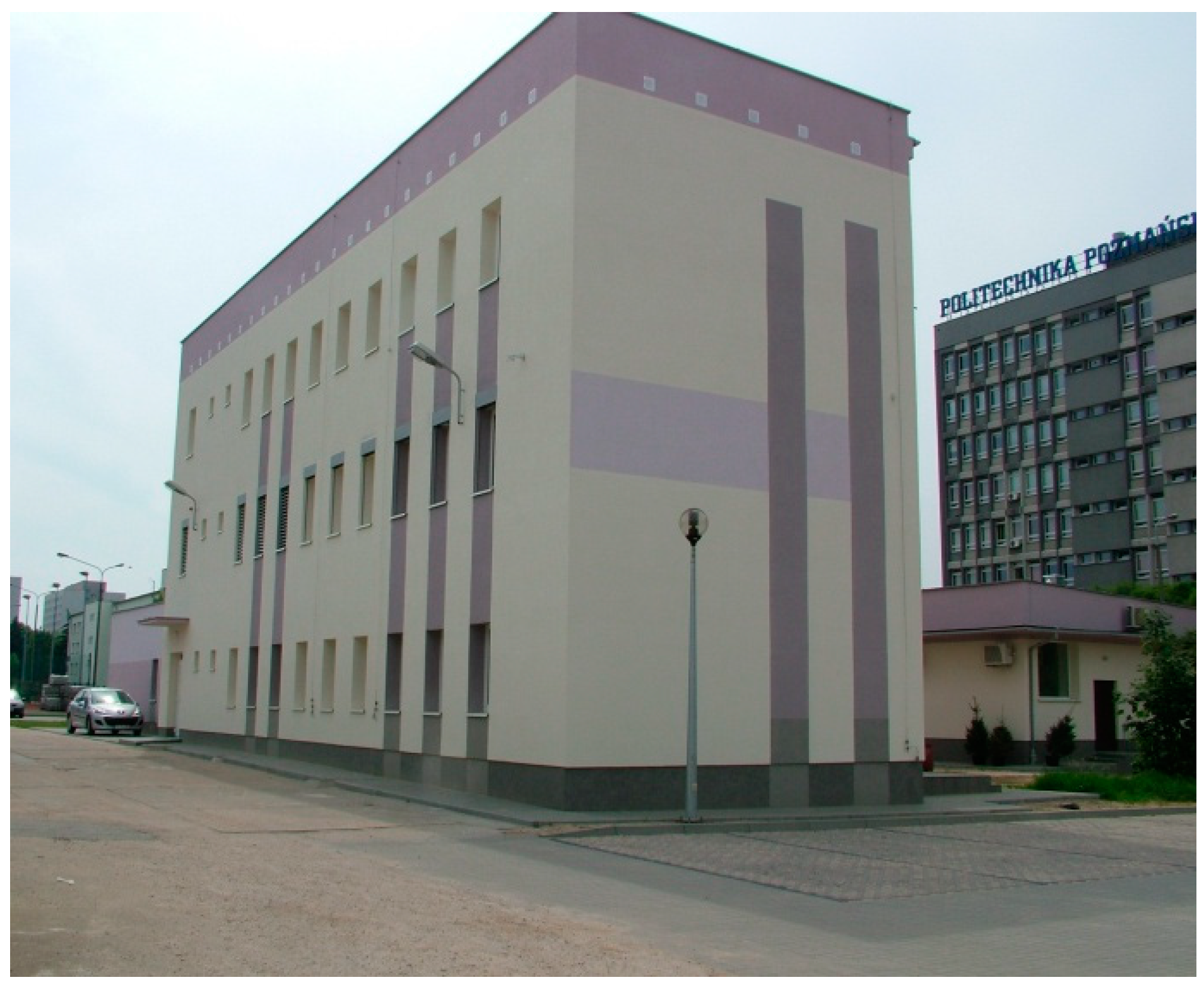
This study deals with the activities of the Laboratory of KNX System and Evolution of Installation Energy Efficiency (SKNX and EIEE Laboratory) at Poznan University of Technology in Poznan, located in the north-western part of Poland (Figure 1). The building was built in the 1980s and is representative of existing Polish buildings from that period considering building envelopes. In 2010 the building was retrofitted and its energy efficiency improved significantly. It is a three-story building with a height of 11.48 m and the external outline surface of 236.8 m2. On the south the building adjoins another facility up to the level of one story.
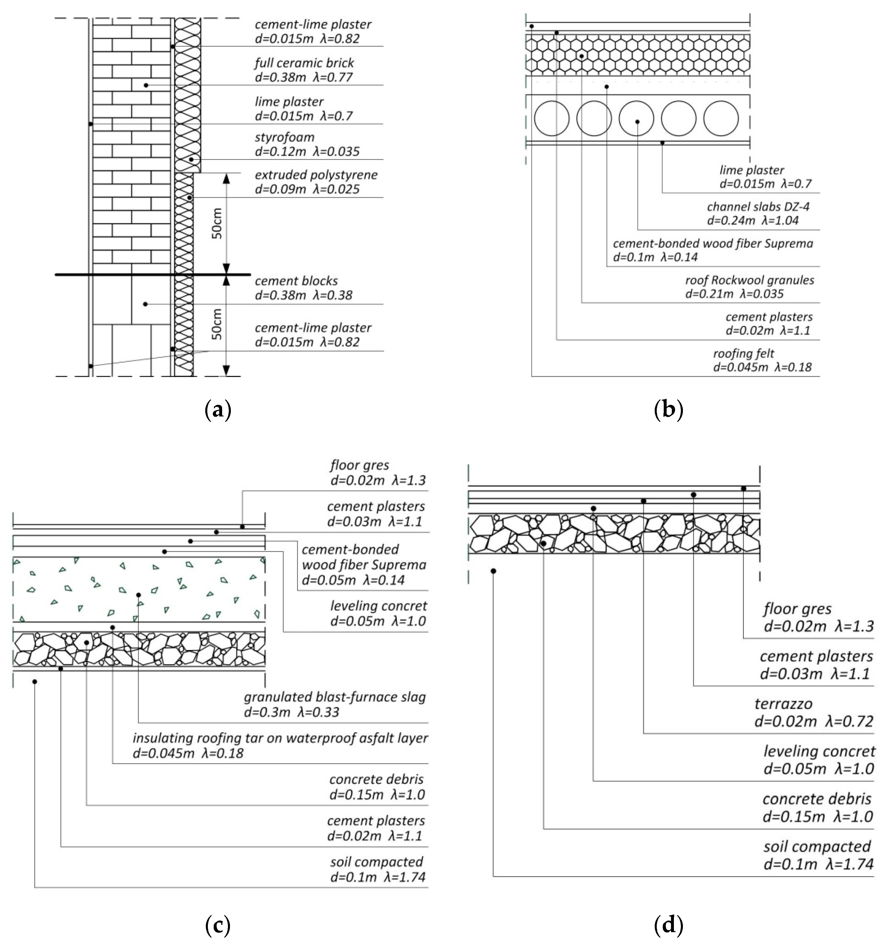
Figure 2 shows the thickness and the value of the thermal conductivity coefficient of each layer that constitutes part of the building envelope. The thermal conductivity coefficients are taken from PN-EN ISO 6946 [37].
The external walls (Figure 2a) with a thickness of 380 mm were built of full ceramic brick and covered with 15 mm lime and cement-lime plasters. In the ground, the walls were made of cement blocks and covered with two 15 mm layers of cement-lime plasters. As a thermal insulation, a 120 mm layer of styrofoam was used on the external walls. At a height of 50 cm below and above the ground, extruded polystyrene with a thickness of 90 mm was placed.
The roof (Figure 2b) is multi-layered and consists of 240 mm channel slabs, 100 mm layer of Supreme, a void of 210 mm, 20 mm cement plaster and the final layer of 45 mm roofing felt. Thermal isolation was achieved by blowing Rockwool granules into the air void. The laboratory floor was not thermo-modernized, and the layers in contact with the ground in the part corresponding to heating zone 1 are presented in Figure 2c, and those corresponding to zones 2 and 3 are shown in Figure 2d. The main layers of the floor in heating zone 1 are a 150 mm layer of concrete debris and a 300 mm layer of granulated blast-furnace slag. Insulating roofing tar on a layer of waterproof asphalt and cement-bonded wood fiber are used as the insulation. In heating zones 2 and 3 the floor forms layers of concrete debris, leveling concrete and terrazzo. The whole floor in all the zones is covered with floor gres laid on cement-plaster.
The thermal resistance of a component layer i of a building envelope is defined as Ri = dii, where di is the thickness of the layer and λi is the thermal conductivity coefficient. The thermal resistance R of a multi-layer building envelope is determined as the sum of the thermal resistance of the component layers and the conventional internal surface thermal resistance Rsi and the external surface thermal resistance Rse. The values of Rsi and Rse resistance depend on the type of building envelope and the direction of heat flow. For external walls and the horizontal direction of heat flow Rsi = 0.13 m2 K/W and Rse = 0.04 m2 K/W, for flat roof Rsi = 0.10 m2 K/W and Rse = 0.04 m2 K/W [38]. The heat transfer coefficient, by definition, is calculated as U = 1/R.
In the walls, there are window jambs, lintels and wall connections, which result in the formation of thermal bridges that increase heat transfer. They are taken into account by introducing a correction of ΔU. For external walls with windows ΔU = 0.05 W/m2 K is assumed.
The heat transfer coefficient for windows is determined as:
U W = A g · U g + A f · U f + l g · Ψ g A g + A f ,
where: Ug and Uf are the heat transfer coefficients in the middle part of double glazing and the frame, respectively, Ag and Af are the surfaces of the glass and the frame, Ψg is the linear heat transfer coefficient of the thermal bridge at the interface between the glass and the frame and lg is the length of the thermal bridge. According to the technical approval for windows Ug = 0.5 W/m2 K and Uf = 1.2 W/m2 K. The surface of the glass is 0.4544 m2 and that of the frame is 0.7781 m2. The length of the thermal bridge amounts to 2.3 m and the linear heat transfer coefficient is taken as 0.06 W/m2 K.
The main entrance to the building leads through two doors from the west. The surface of the single door is 3.494 m2. There is an additional door with a surface of 3.478 m2 on the east of the building, occasionally used for moving heavy equipment. According to the technical approval the heat transfer coefficient is 2.6 W/m2 K.

3.2. Heating Zones

The building was divided into heating zones shown in Figure 3, differing in use, size and separation walls. The division into zones determined the pipeline system, in particular the number of heating circuits supplying hot water to panel radiators.
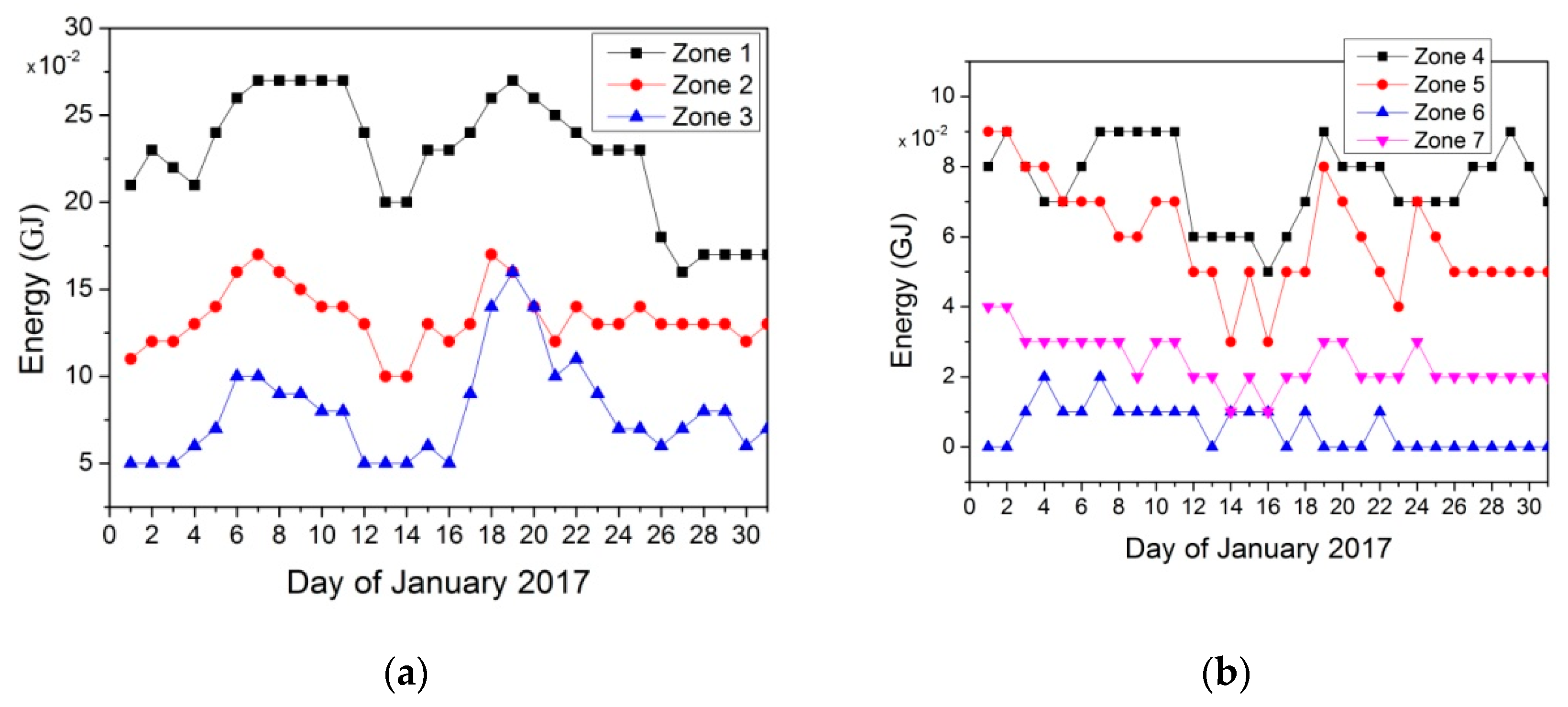
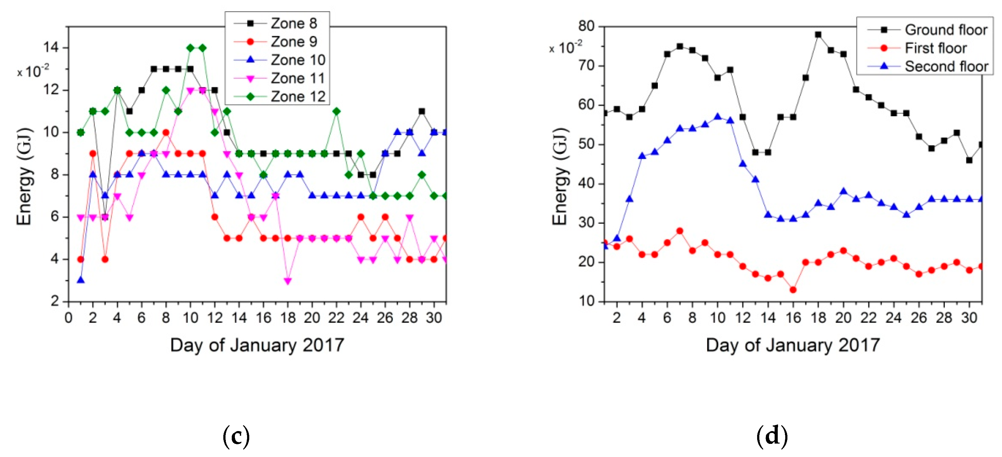
On the ground floor, there are three heating zones, namely zone 1 and 2 including high-current laboratories and zone 3 including a workshop, sanitary facilities and a corridor. People staying in these rooms do not perform sedentary work and the operation of the devices causes an increase in temperature. The first floor consists of four heating zones. These zones are the most stable in temperature, due to the floor being closed with a staircase door and because of its location between the heated floors of the building. The second floor was divided into five heating zones corresponding to the rooms. The height of all zones is the same and amounts to 2.8 m.

3.3. Control System and Data Acquisition

The heating system in the SKNX and EIEE Laboratory building is designed in such a way that it is possible to estimate the heat consumption in each room and implement various control algorithms as well as to measure, record and visualize useful data [
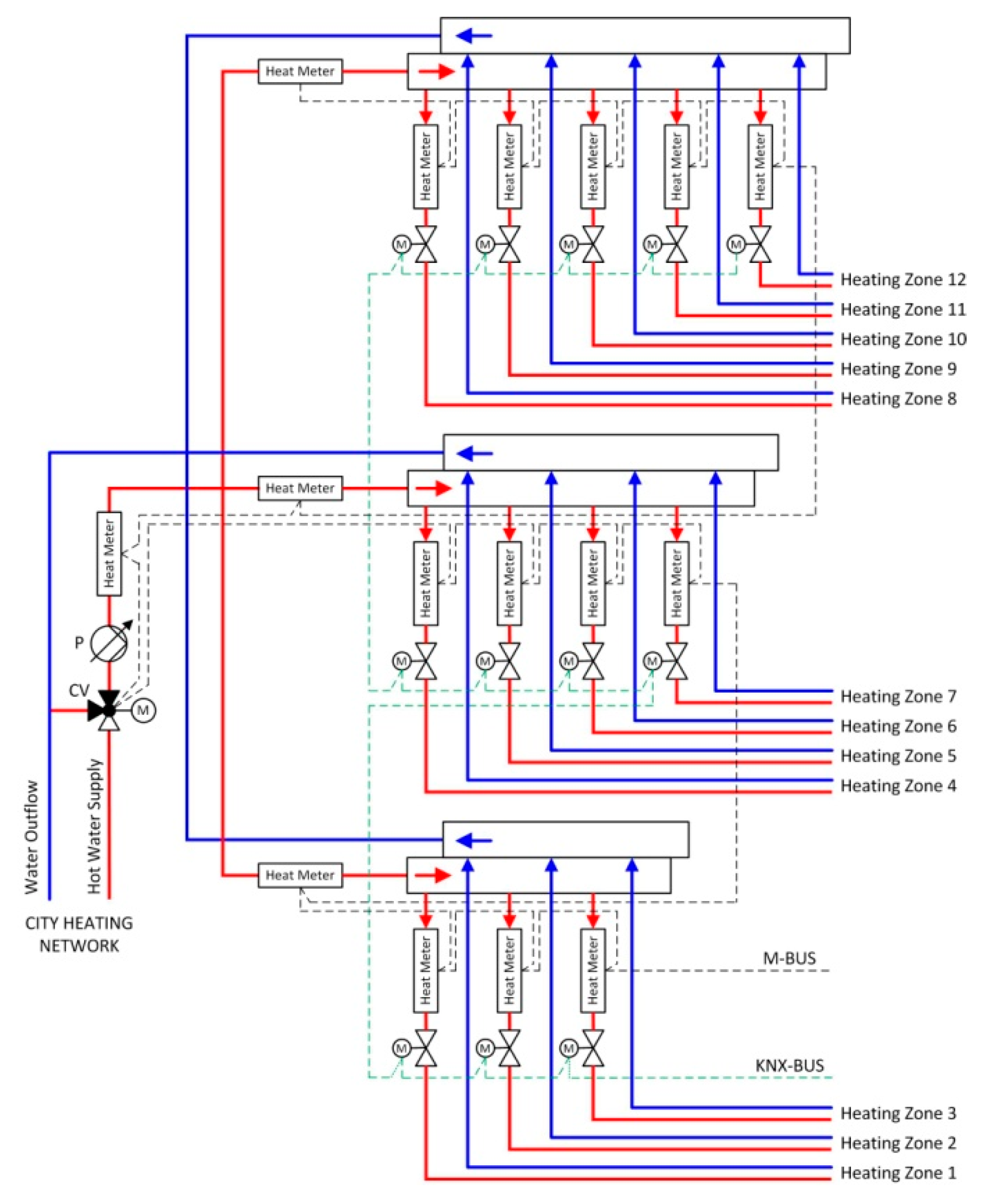
39]. Panel radiators are used as the heating devices. In this system heat is carried by water supplied from the city heating network. The scheme of the pipeline system is shown in Figure 4. In order to force the water flow through the installation, circulation pump (P) is used. At the inflow, a control valve (CV) has been mounted and heating water parameters are measured using a heat meter. Then, the hot water flows into three main circuits assigned to each story and the heating water parameters are also measured at the inflow to each circuit. The water feeds heating circuits assigned to heating zones (Figure 3): on the ground floor—three circuits, on the first floor—four circuits and on the second floor—five circuits. Water from heating devices returns through the pipelines on the stories and then the main pipeline to the city heating network. Each water circuit is equipped with a heat meter and a KNX servo drive. The servo drives are controlled by signals sent directly from the KNX bus. The KNX multi-function push-button with a room temperature control unit is located in each heating zone. In addition, the KNX Laboratory (heating zone 5) is equipped with a KNX touch panel that visualizes the states and parameters of the system. A valve controller at the heating system inflow and heat meters is connected to the ControlMaestro controller with a SCADA (superior control and data acquisition) system using an M-Bus network (Figure 4). This system allows the visualization and acquisition of values measured in the building heating system.
To control the heating system KNX devices mentioned above and KNX BACS field network are used. In the KNX system other devices are integrated, including a weather station, brightness and temperature sensor, presence detectors and Gira HomeServer. KNX is an open standard for public, commercial and domestic buildings [40], which allows the integration of many devices from different manufacturers. KNX devices are most often connected by a twisted pair or RF bus and programmed with the use of ETS software. It is worth noting that the system used in the laboratory building can be easily expanded with new devices, and in addition, it allows testing various control algorithms through reprogramming using the available ETS software. Two networks, M-Bus and KNX, are integrated using a M-Bus/KNX converter (Figure 5), which enables the acquisition of all measured values and events in the form of telegrams (standardized KNX messages) by the KNX HomeServer. The HomeServer visualizes the results on-line, archives them and, once a day, sends the results as a csv file to specified e-mail addresses. The recording format allows further processing of the results by external tools and programs.
The following data were recorded by the HomeServer:
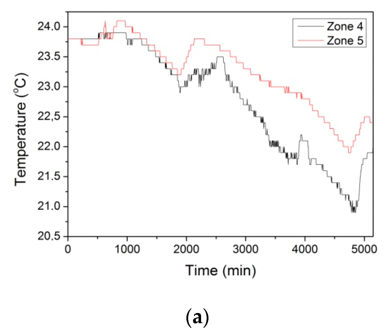
  • Set point and current temperature in each heating zone from a push-button with room temperature control unit, measured with the accuracy of ±1 °C (logged every 5 min);
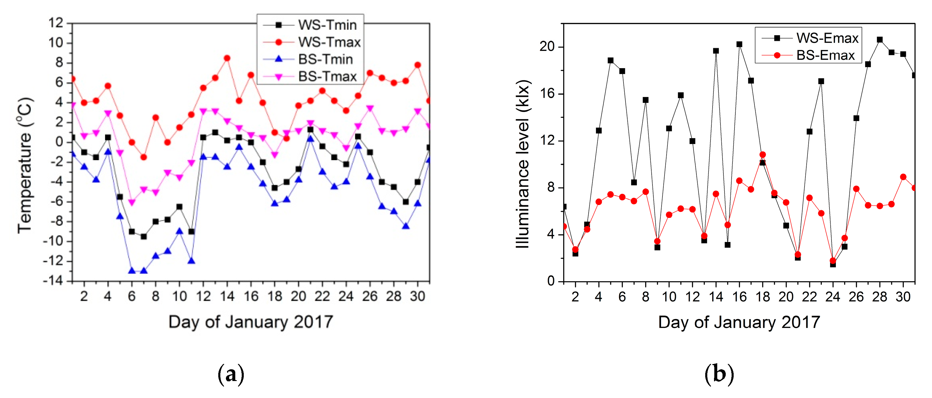
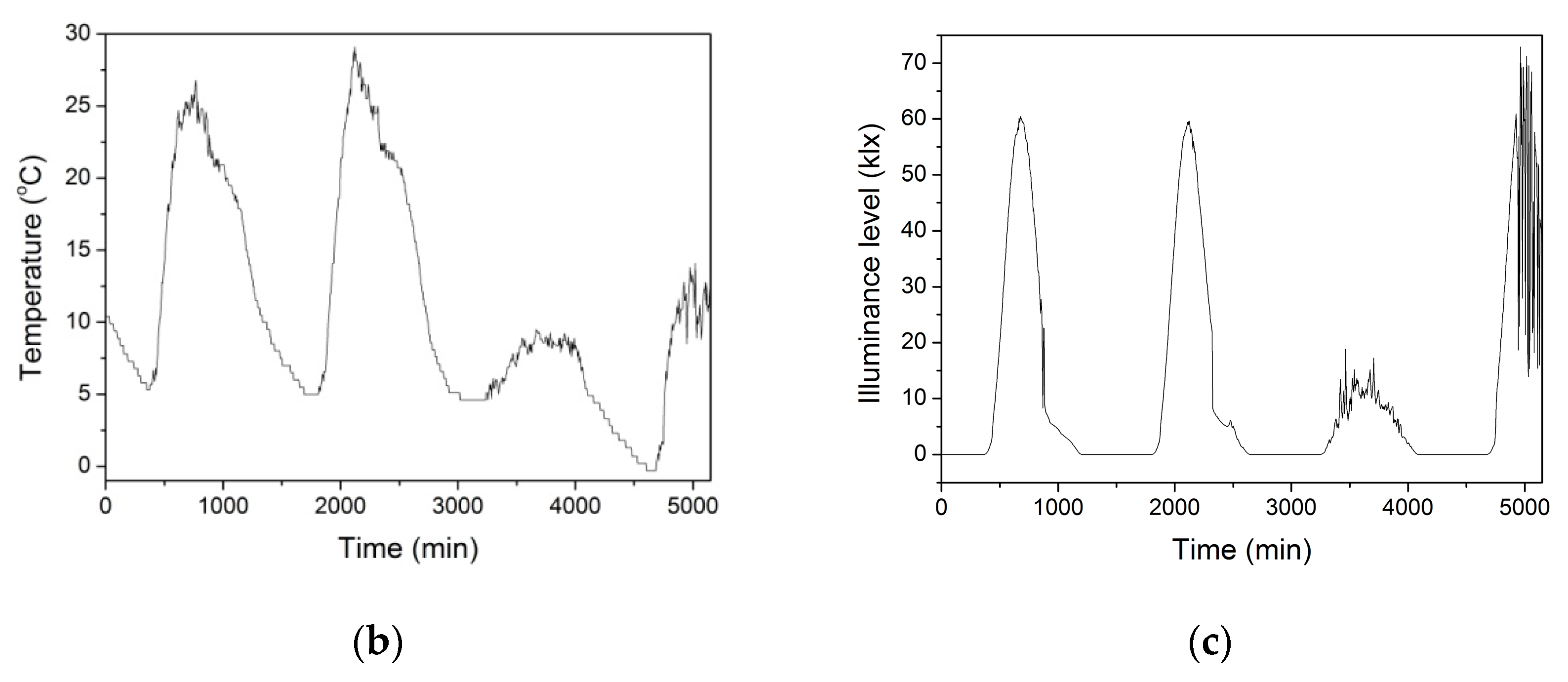
  • Temperature from the weather station and the external brightness and temperature sensor mounted on the building facades, measured with the accuracy of ±1 °C (logged every 5 min);
  • Wind speed from the weather station, measured with the accuracy of ±1.5 m/s (logged every 5 min);
  • Occurrence (or absence) of rainfall or snowfall from the weather station (logged every 5 min);
  • Illuminance level, from the weather station and the external brightness and temperature sensor, measured with the accuracy of ±5 lux (logged every 5 min);
  • Energy from the heat meters, measured with the accuracy of ±5% (logged every 30 min);
  • Instantaneous power from the heat meters, measured with the accuracy of ±5% (logged every 5 min);
  • Position status of the windows in each room.
In order to determine the position status of the windows and take it into account in the heating control, the intruder alarm system (IAS) in the building was integrated with the KNX system. In window frames, reed switches are mounted and signals from these devices are sent to the alarm control unit, which transmits them to the KNX binary input.

3.4. Temperature Set Point

The temperature set points for the heating seasons are established based on ISO (International Standard Organization) Standard 7730 [41], which defines the comfort ranges according to the specificity of Europe [42]. However, it should be noted that thermal sensations differ between persons sharing the same environment, because there are many factors that affect the perception of human beings [26,28]. The thermal sensations experienced by a human being result mainly from the overall thermal balance of the body. This balance includes two components, namely heat generated by a human being and heat transferred to the environment. The first depends on the physical activity and the second depends on clothing, as well as on environmental parameters such as air temperature, radiant temperature, air velocity and air humidity [43].
The American Society of Heating, Refrigerating and Air-Conditioning Engineers (ASHRAE) standard [44] specifies the conditions in which a fraction of occupants find the environment thermally acceptable. The predicted mean vote (PMV) and the predicted percentage dissatisfied (PPD) are defined in ISO 7730 [41]. The thermal comfort index PMV-PPD reflects the degree of human thermal balance deviation and is a comprehensive comfort indicator that represents the feelings of most people in the same environment. PMV scales constitute seven thermal sensation points ranging from −3 (cold) to +3 (hot), where 0 means a neutral thermal sensation [45]. The PMV index involves activities (expressed through the metabolic rate index), clothing corresponding to the total thermal resistance from the skin to the outer surface of the clothed body and the four environmental parameters mentioned above [41,46].
Depending on the admissible ranges for PMV and PPD, three kinds of comfort zones or categories of thermal requirements are defined by ISO 7730 as: category I (or class A; PPD < 6%, i.e., −0.2 < PMV < 0.2), category II (or class B; PPD < 10%, i.e., −0.5 < PMV < 0.5) and category III (or class C; PPD < 15%, i.e., −0.7 < PMV < 0.7). The ranges of recommended air temperatures for different types of buildings depending on the previous categories are shown in Table 1 [41]. Thus, in the study case building the range of temperature set point was set from 19 to 25°C and the occupant had some freedom to choose the preferred temperature during their presence in the room. It should be noted that this value was a subjective decision of the occupant and the prediction of occupant behavior was a factor of considerable uncertainty in the analysis [47].

3.5. Building Use and Heating Control Algorithm

The analyzed information about the occupancy, opening windows, operation mode of the heating system and changing the temperature set point in each room of the building is derived from the data recorded by Gira HomeServer. On weekdays, the building is usually occupied from 8 a.m. to 6 p.m. In this time, the heating system operates in comfort mode with the various temperature set points in the rooms set by the occupants. From 6 p.m. to 8 a.m. the system operates in night mode with the constant temperature of 16 °C. In practice, lowering the temperature set point to 16 °C results in closing the KNX servo drive and switching off the heating system. This control algorithm is considered below and the experimental results were compared with the calculation. To assess the energy saving potential due to heating control the same algorithm was assumed, but the temperature was constant in comfort mode (21 or 20 °C). This case was referred as “with control”.
In a real heating control other functions are implemented. One of these functions is the detection of window opening (or tilling from the top by 30° from vertical). This function is essential because the occupants have free and easy access to open the windows in their own office and laboratory rooms. Opening the window by the user in the room results in a transition of the heating system to the anti-frost mode with a temperature of 7 °C. In addition, the heating control system was integrated with the intruder alarm system. It is not possible to arm this system when a window in the building is open. Occupants leaving the building arm the system and they must close all the windows.
Another function is presence detection in the off time, between 6 p.m. and 8 a.m. and on weekends. If users start work earlier, finish later or work on weekends, information about the events is transmitted from the presence sensor to the heating control system, which changes the operating mode to comfort mode in the room where such presence is detected.

4. Calculation of Energy Consumption

The energy consumption Qsmj in the time interval Δtm in the j-th heating zone is estimated taking into account heat transfer through the building envelope and heat losses for ventilation according to the following formula [14,15]:
Q s m j = i = 1 n Q T i j + Q V j ,
where: QTij is heat losses for transmission through the i-th barrier in the j-th heating zone, QVj is heat losses for ventilation in the j-th heating zone and n is the number of partitions.
The heat losses (or gains) for transmission through the i-th barrier are estimated as:
Q T i = U i · ( ϑ i m ϑ e i m ) · A i · Δ t m ,
where: Ui is the heat transfer coefficient through the i-th barrier in W/m2 K, ϑim is the air temperature in °C, in the room, in the time interval Δtm, ϑeim is the air temperature in °C, outside the i-th barrier, in the time interval Δtm, Ai is the surface of the i-th barrier in m2 and Δtm is the time interval in hours.
The heat loss for ventilation in the j-th heating zone in Wh is calculated as follows:
Q V j = 0.333 · ( ϑ i m ϑ e i m ) · V j · Δ t m ,
where: Vj is the ventilation air stream flowing into the j-th heating zone in m3.
Ventilation of the rooms is provided by ventilation ducts (Figure 3) and window ventilators integrated in the frames. Each ventilator is equipped with a regulator allowing different air flow rates. Due to the impact of various parameters on the performance of natural ventilation and the complexity of the phenomenon [16,17,18,19], the volume of ventilated air in the room was estimated based on the difference between energy consumption measured with open window ventilators and this energy measured with completely closed ventilators and ventilation duct. This difference determines the heat loss for ventilation and the volume Vj is estimated using Formula (4).
Energy consumption in the analyzed period is estimated as the sum of heat losses calculated in time intervals m in which various temperature increases ϑim − ϑeim occurred, therefore:
Q s j = m Q s m j .

5. Results and Discussion

5.1. Ambient Weather Temperature and Daylight Illuminance

The analysis of energy consumption was carried out for the month of January 2017. January is usually the coldest month of the year in Poland. The calculations were performed taking into account the actual ambient temperature measured by the weather station installed on the south-eastern facade of the building. In calculation it is ϑeim temperature. However, the temperature was also measured by the external brightness and temperature sensor mounted on the northern facade. It should be noted that the values measured by these two sensors on a sunny day differ from each other. Two phenomena are responsible for the measurement discrepancies. The first one is the insolation of the building walls, which is stronger for the south-eastern wall than for the north wall. On cloudy days there is no difference in the heating of the walls by sunlight and the measured temperatures are close to each other. The second is the direct impact of sunlight on the weather station. This effect is mainly observed on a sunny day with high variability of daylight. In this case, variations in illuminance and temperature occur simultaneously. The lowest and highest temperatures on each day of January measured by the weather station and the brightness sensor are shown in Figure 6a. The lowest temperature in the month was about −13 °C and the highest about 4 °C. The temperature difference during the day reached 10 °C.
When the illuminance levels measured by the weather station and the brightness sensor are the same (Figure 6b), it means that the day is overcast and the walls are not heated by sunlight. This is from 18 to 21 January. Obviously, there is a time shift between variations in the illuminance level and the temperature. On 18 January, the wall was still warmed up by daylight and there was a difference in the measured temperature values. Due to these temperature differences, on a sunny day, the temperature values measured by the brightness and temperature sensor are represented as ϑeim temperature in the calculation. Time intervals Δtm are determined, in which the temperature ϑeim differs by 1 °C. The air temperature ϑim is taken as the current temperature in the heating zone, measured by the push-button with room temperature control unit and recorded by the HomeServer.

5.2. Temperature Changes Inside the Building

The implementation of heating control algorithms must take into account temperature changes in the rooms as a result of lowering the temperature set point, switching off the heating, opening the window and other events. Anyway, heating control usually consists in lowering the temperature at night and on weekends and turning off the heating after opening the window. The change in temperature will depend on the thermal properties of the building and the ambient conditions, i.e., temperature, wind speed, rainfall and daylight. Figure 7a shows the temperature inside and Figure 7b the temperature outside the building during three days, i.e., from 0:00 on 10 April to 24:00 on 12 April, which is during 4320 min. To investigate temperature changes in the building, the temperature was first lowered by fully opening (on 9 April) one window in zones 4 and 5. The heating system switched to the anti-frost mode and until 9:40 on 10 April (in 580 min) the temperature in these zones decreased to 20.9 and 21.8 °C, respectively. At that time, the windows were closed and the temperature increased to the temperature set points. Further temperature changes were forced at 18:40 (in 1120 min) by turning the heating system off and then at 9:30 on 12 April (in 3450 min) by turning this system on. Temperature changes in zone 4 prove the high thermal inertia of this zone and it may take several hours to reach a higher temperature set point or comfort mode temperature after earlier turning off the heating. On the other hand, the temperature reduction after switching off the heating is small when the windows are closed. For the considered conditions it was approximately 1 °C for about 39 h. It is worth noting that the temperature changes in zone 4 were even smaller than in zone 5. In zone 3 the window was not open and the temperature increased around 750 and 2100 min as a results of insolation and an increase of temperature outside the building. A slight effect of the outside temperature on the inside temperature could also be seen in zones 4 and 5.
In order to estimate the effect of window operation on energy consumption, the temperature changes after tilting the window from the top by 30° from vertical were analyzed. It is worth noting that such window operation was often used by occupants. The window was tilted on 6 April at 16:15, 975 min from 0, which corresponds to 0:00. Figure 8a shows that after tilting the windows the temperature in both zones dropped to about 23 °C, then due to the increase in the outside temperature (Figure 8b) the temperature inside the zones increased too. However, the temperature increase in the two zones was different due to the difference in insolation of these rooms. In zone 4 the windows were located on one wall of the room on the north-east side, while in zone 5, the windows were on two sides of the room, i.e., north-west and north-east. The illuminance level of daylight is shown in Figure 8c.
On 8 April, the daytime temperature dropped below 10 °C and then to around −1 °C at night. This resulted in a lower room temperature, more significant in zone 4. On 9 April at 9:40 (4900 min) the windows were closed in both zones, the heating system turned on and the temperature started increasing to the set point value. It should be noted that tilting of only one window in the room led to a temperature decrease of around 3 °C during the considered time, which corresponds to the weekend time.

5.3. Energy Consumption Experiment and Calculation

Energy consumption in the heating zones on days of January 2017, measured by the heat meters, is shown in Figure 9, and Table 2 presents the measured and calculated energy consumed over the whole month. The results were obtained with no heating control and the actual room temperatures were equal to the temperature set points. The occupants had the freedom to choose the temperature set points and, as can be seen in Table 2, the range of the selected set points was wide: from 19 to 24.5 °C. It reveals a strong influence of individual occupant preferences on the feeling of comfort.
The highest energy consumption (Figure 9a) was in heating zone 1 due to the large volume of air to be heated, which results from the fact that this zone includes not only the laboratory room but also the entrance of the building and the open space of the staircase. The energy consumption in heating zone 2 was higher than in zone 3 due to the heat transfer through the door in zone 2 and a lower temperature in zone 3. The comparison of energy consumption on the three floors of the building (Figure 9d) shows that the highest consumption was on the ground floor due to the poor thermal insulation of the floor and the volume of heated air. The lowest energy consumption occurred in the rooms on the first floor (Figure 9b). On the second floor, where there was heat transfer through the roof, energy consumption was higher than on the first floor.
Energy consumption in each room depended on their volume, temperature set point and insolation, therefore it was better to compare the energy consumption per unit of room area, at which the above conclusions were rather obvious. Another good example is the comparison of energy consumption per unit of room area in heating zones 4 and 8 with the same volume, which showed that the consumption in zone 4 was lower despite a higher temperature. It is worth noting that the calculated value was always larger than the measured value, and it seemed to be the case for two reasons. Firstly, heat gains from insolation, people and equipment were not included in the calculations. Secondly, at small energy values measured, heat meter indications were burdened with significant errors, namely the values were underestimated. As the measurement of thermal energy by the heat meter was carried out indirectly, on the basis of measuring the volume of the water and the temperature difference at the inflow and return, the measurement error could be relatively large (±5%). However, the difference between the calculated and measured energy consumption values in relation to the measured value did not exceed 15% and the estimation of energy consumption could be considered sufficiently accurate.

5.4. Effect of Room Temperature and Heating Control on Energy Consumption

In the heating season 2017/2018, between the end of September and the beginning of May, time control of the heating was implemented. Due to different weather conditions, the experimental results of two heating seasons could not be compared in order to estimate the effect of heating control on the reduction of energy consumption. Therefore, the calculations were carried out for the weather conditions in January 2017: first, without heating control, assuming that the room temperature was 21 and 20 °C. The value of 21 °C corresponds to the recommended indoor air temperature in education rooms of category A and 20 °C in rooms of category B (Table 1). Then, based on the observation, it was assumed that after the transition of the heating system to night mode, the temperature dropped in the rooms located on the ground floor by an average of 1.5 °C at night (during 14 h). At weekends (during 62 h), the reduction was about 4 °C. These temperature drops were, respectively, about 0.5 °C and 1.5 °C in the rooms on the first floor and 1 °C and 3 °C on the second floor. The calculation results are given in Table 3. This calculation shows that reducing the temperature set point by 1 °C gives an energy saving of about 5% compared to energy consumption at 21 °C.
The comparison of energy consumption with and without heating control reveals that the energy saving potential mainly depended on the temperature drop after the set point lowering. The greater the decrease, the greater the potential for energy savings. In the study case, in the rooms with a poorly heat-insulated floor, the energy reduction due to heating control reached about 10%. A slightly lower reduction of about 7.5% was estimated for the rooms on the second floor, where heat was transferred through the roof, and the smallest reduction of less than 4% was estimated for the rooms on the first floor. This proves that in well-insulated rooms with a low energy consumption for heating the implementation of the control system gave relatively little benefit.
For energy saving, a very important function was to control the opening of a window. As shown in Figure 8 the tilt of the top of only one window in the room led to a temperature decrease of a few degrees. Leaving the window open before night or weekend would result in a significant increase in energy consumption, by about 5% per 1 °C drop.

6. Conclusions and Future Work

In this paper, the potential of energy savings in an existing public building in Poland was estimated. This estimation includes the most important parameters affecting energy consumption for heating. Experimental verification of the building case study showed that the calculation of energy consumption in a cold climate including the heat transfer through the building envelope and heat losses for ventilation were sufficiently accurate. In such calculations, a good knowledge of the thermal characteristics of the building, the volume of ventilated air and the temperature outside and inside the building is crucial.
Using the KNX system implemented in the building, the behavior of occupants was investigated revealing that occupants choose temperature set points in a wide range recognized as thermal comfort, and window opening was also accidental and difficult to predict. The proposed heating control algorithms took into account the strong influence of individual occupant preferences on the feeling of comfort. However, in order to reduce energy consumption, the anti-frost mode was applied after opening the window, as well as integration with the intruder alarm system. Investigation of temperature changes in the building with changes in the temperature set points and after opening the window showed that from the point of view of energy saving, the most important issue is the window opening control.
Finally, detailed comparisons of energy consumption with heating control and without any controls were performed. It shows that the energy saving potential depended on the temperature drop after lowering the set point, and thus on the dynamics of the thermal behavior of the building. The greater this drop, the greater the potential for energy savings. In the case study, in rooms with poorly heat-insulated floors, the energy reduction potential due to heating control reached about 10%. A slightly lower potential of about 7.5% was estimated for rooms on the second floor, where heat was transferred through the roof, and the smallest potential of less than 4%, for rooms on the first floor. This proved that in a well-insulated room with a low energy consumption for heating, the implementation of the control system gave relatively little benefit.
Future work will include an analysis of information from presence detectors to describe occupant behavior, and the implementation of such information to control heating and estimate energy savings. Research associated with the optimal operation of the heat source will also be undertaken.

Funding

This study is based upon work supported by the National Centre for Research and Development in the context of the Innovative Economy Program under grant No. POIG.02.02.00-00-018/08. This work was also supported by the 2018 Poznan University of Technology funds transferred from the Ministry of Science and Higher Education.

Conflicts of Interest

The author declares no conflict of interest. The funders had no role in the design of the study; in the collection, analyses, or interpretation of data; in the writing of the manuscript, and in the decision to publish the results.

References

  1. International Energy Agency (IEA). Key World Energy Statistics; International Energy Agency (IEA): Paris, France, 2018. [Google Scholar]
  2. Energy Information Administration (EIA). Energy Consumption by Sector; U.S. Department of Energy: Washington, DC, USA, 2019.
  3. European Commission. Consumption of Energy; European Commission: Brussels, Belgium, 2019. [Google Scholar]
  4. European Commission. Driving Energy Efficiency in the European Building Stock: New Recommendations on the Modernisation of Buildings; European Commission: Brussels, Belgium, 2019. [Google Scholar]
  5. European Parliament and of the Council. Directive EU 2018/844 of the European Parliament and of the Council of 30 May 2018 Amending Directive 2010/31/EU on the Energy Performance of Buildings and Directive 2012/27/EU on Energy Efficiency; Official Journal of the European Union: Brussels, Belgium, 2018. [Google Scholar]
  6. Ma, Z.; Cooper, P.; Daly, D.; Ledo, L. Existing building retrofits: Methodology and state-of-the-art. Energy Build. 2012, 55, 889–902. [Google Scholar] [CrossRef]
  7. Najjar, M.K.; Tam, V.W.Y.; Di Gregorio, L.T.; Evangelista, A.C.J.; Hammad, A.W.A.; Haddad, A. Integrating Parametric Analysis with Building Information Modeling to Improve Energy Performance of Construction Projects. Energies 2019, 12, 1515. [Google Scholar] [CrossRef]
  8. Allouhi, A.; El Fouih, Y.; Kousksou, T.; Jamil, A.; Zeraouli, Y.; Mourad, Y. Energy consumption and efficiency in buildings: current status and future trends. J. Clean. Prod. 2015, 109, 118–130. [Google Scholar] [CrossRef]
  9. Pérez-Lombard, L.; Ortiz, J.; Pout, C. A review on buildings energy consumption information. Energy Build. 2008, 40, 394–398. [Google Scholar] [CrossRef]
  10. Chen, Z.; Jiang, C.; Xie, L. Building occupancy estimation and detection: A review. Energy Build. 2018, 169, 260–270. [Google Scholar] [CrossRef]
  11. Gul, M.S.; Patidar, S. Understanding the energy consumption and occupancy of a multi-purpose academic building. Energy Build. 2015, 87, 155–165. [Google Scholar] [CrossRef]
  12. Zhao, H.; Magoulès, F. A review on the prediction of building energy consumption. Renew. Sustain. Energy Rev. 2012, 16, 3586–3592. [Google Scholar] [CrossRef]
  13. Wang, S.; Yan, C.; Xiao, F. Quantitative energy performance assessment methods for existing buildings. Energy Build. 2012, 55, 873–888. [Google Scholar] [CrossRef]
  14. EN ISO 13790. Energy Performance of Building—Calculation of Energy Use for Space Heating and Cooling; European Committee for Standardization (CEN): Brussels, Belgium, 2008. [Google Scholar]
  15. Gładyszewska-Fiedoruk, K.; Krawczyk, D.A. The possibilities of energy consumption reduction and a maintenance of indoor air quality in doctor’s offices located in north-eastern Poland. Energy Build. 2014, 85, 235–245. [Google Scholar] [CrossRef]
  16. Sacht, H.; Lukiantchuki, M.A. Windows Size and the Performance of Natural Ventilation. Procedia Eng. 2017, 196, 972–979. [Google Scholar] [CrossRef]
  17. Zhai, Z.; El Mankibi, M.; Zoubir, A. Review of Natural Ventilation Models. Energy Procedia 2015, 78, 2700–2705. [Google Scholar] [CrossRef]
  18. Shetabivash, H. Investigation of opening position and shape on the natural cross ventilation. Energy Build. 2015, 93, 1–15. [Google Scholar] [CrossRef]
  19. Bangalee, M.Z.I.; Lin, S.Y.; Miau, J.J. Wind driven natural ventilation through multiple windows of a building: A computational approach. Energy Build. 2012, 45, 317–325. [Google Scholar] [CrossRef]
  20. Gunay, B.; O’Brien, W.; Morrison, I.B. A critical review of observation studies, modelling and simulation of adaptive occupant behaviours in offices. Build. Environ. 2013, 70, 31–47. [Google Scholar] [CrossRef]
  21. McCartney, K.J.; Nicol, J. Developing an adaptive control algorithm for Europe. Energy Build. 2002, 34, 623–635. [Google Scholar] [CrossRef]
  22. Nicol, J.F.; Humphreys, M.A. Adaptive thermal comfort and sustainable thermal standards for buildings. Energy Build. 2002, 34, 563–572. [Google Scholar] [CrossRef]
  23. Toe, D.H.C.; Kubota, T. Development of an adaptive thermal comfort equation for naturally ventilated buildings in hot–humid climates using ASHRAE RP-884 database. Front. Archit. Res. 2013, 2, 278–291. [Google Scholar] [CrossRef]
  24. Nguyen, A.T.; Singh, M.K.; Reiter, S. An adaptive thermal comfort model for hot humid South-East Asia. Build. Environ. 2012, 56, 291–300. [Google Scholar] [CrossRef]
  25. Rinaldi, A.; Schweiker, M.; Iannone, F. On uses of energy in buildings: Extracting influencing factors of occupant behaviour by means of a questionnaire survey. Energy Build. 2018, 168, 298–308. [Google Scholar] [CrossRef]
  26. Rupp, R.F.; Vásquez, N.G.; Lamberts, R. A review of human thermal comfort in the built environment. Energy Build. 2015, 105, 178–205. [Google Scholar] [CrossRef]
  27. Fanger, P. Thermal Comfort; McGraw-Hill: New York, NY, USA, 1973. [Google Scholar]
  28. Robledo-Fava, R.; Hernández-Luna, M.C.; Fernández-de-Córdoba, P.; Michinel, H.; Zaragoza, S.; Castillo-Guzman, A.; Selvas-Aguilar, R. Analysis of the Influence Subjective Human Parameters in the Calculation of Thermal Comfort and Energy Consumption of Buildings. Energies 2019, 12, 1531. [Google Scholar] [CrossRef] [Green Version]
  29. Yu, Z.; Fung, B.C.M.; Haghighat, F.; Yoshino, H.; Morofsky, E. A systematic procedure to study the influence of occupant behaviour on building energy consumption. Energy Build. 2011, 43, 1409–1417. [Google Scholar] [CrossRef] [Green Version]
  30. Yan, D.; OBrien, W.; Hong, T.; Feng, X.; Gunay, H.B.; Tahmasebi, F.; Mahdavi, A. Occupant behaviour modeling for building performance simulation: current state and future challenges. Energy Build. 2015, 107, 264–278. [Google Scholar] [CrossRef] [Green Version]
  31. Shih, H.C. A robust occupancy detection and tracking algorithm for the automatic monitoring and commissioning of a building. Energy Build. 2014, 77, 270–280. [Google Scholar] [CrossRef]
  32. Dong, J.; Winstead, C.; Nutaro, J.; Kuruganti, T. Occupancy-Based HVAC Control with Short-Term Occupancy Prediction Algorithms for Energy-Efficient Buildings. Energies 2018, 11, 2427. [Google Scholar] [CrossRef] [Green Version]
  33. Wang, F.; Feng, Q.; Chen, Z.; Zhao, Q.; Cheng, Z.; Zou, J.; Zhang, Y.; Mai, J.; Li, Y.; Reeve, H. Predictive control of indoor environment using occupant number detected by video data and CO2 concentration. Energy Build. 2017, 145, 155–162. [Google Scholar] [CrossRef]
  34. Lee, S.; Jung, S.; Lee, J. Prediction Model Based on an Artificial Neural Network for User-Based Building Energy Consumption in South Korea. Energies 2019, 12, 608. [Google Scholar] [CrossRef] [Green Version]
  35. Brastein, O.M.; Perera, D.W.U.; Pfeifer, C.; Skeie, N.O. Parameter estimation for grey-box models of building thermal behaviour. Energy Build. 2018, 169, 58–68. [Google Scholar] [CrossRef] [Green Version]
  36. Berthou, T.; Stabat, P.; Salvazet, R.; Marchio, D. Development and validation of a gray box model to predict thermal behaviour of occupied office buildings. Energy Build. 2014, 74, 91–100. [Google Scholar] [CrossRef]
  37. PN-EN ISO 6946. Komponenty Budowlane i Elementy Budynku—Opór Cieplny i Współczynnik Przenikania Ciepła—Metoda Obliczania; Polski Komitet Normalizacyjny: Warsaw, Poland, 2008. [Google Scholar]
  38. PN-EN ISO 10211. Mostki Cieplne w Budynkach. Strumienie Ciepła i Temperatury Powierzchni. Obliczenia Szczegółowe; Polski Komitet Normalizacyjny: Warsaw, Poland, 2008. [Google Scholar]
  39. Kaminska, A.; Ożadowicz, A. Lighting Control Including Daylight and Energy Efficiency Improvements Analysis. Energies 2018, 11, 2166. [Google Scholar] [CrossRef] [Green Version]
  40. KNX Association. Handbook for Home and Building Control, Basic Principles, 5th ed; KNX Association: Brussels, Belgium, 2006. [Google Scholar]
  41. Standard 7730. Ergonomics of the Thermal Environment—Analytical Determination and Interpretation of Thermal Comfort Using Calculation of the PMV and PPD Indices and Local Thermal Comfort Criteria; International Organization for Standardization: Geneva, Switzerland, 2005. [Google Scholar]
  42. CEN. 15251-Criteria for the Indoor Environment, Including Thermal, Indoor Air Quality (Ventilation), Light And Noise; CEN: Brussels, Belgium, 2006. [Google Scholar]
  43. Fanger, P.O. Thermal environment—Human requirements. Environmentalist 1986, 6, 275–278. [Google Scholar] [CrossRef]
  44. ASHRAE. ANSI/ASHRAE Standard 55-2010: Thermal Environmental Conditions for Human Occupancy; American Society of Heating, Refrigerating and Air-Conditioning Engineers: Atlanta, GA, USA, 2010. [Google Scholar]
  45. Fanger, P.O. Thermal Comfort. In Analysis and Applications in Environmental Engineering; Danish Technical Press: Copenhagen, Denmark, 1970. [Google Scholar]
  46. Antoniadou, P.; Papadopoulos, A.M. Occupants’ thermal comfort: State of the art and the prospects of personalized assessment in office buildings. Energy Build. 2017, 153, 136–149. [Google Scholar] [CrossRef]
  47. Hong, T.; Taylor-Lange, S.C.; D’Oca, S.; Yan, D.; Corgnati, S.P. Advances in research and applications of energy-related occupant behaviour in buildings. Energy Build. 2016, 116, 694–702. [Google Scholar] [CrossRef] [Green Version]
Figure 1. External view of the KNX System and Evolution of Installation Energy Efficiency (SKNX and EIEE) Laboratory building.
Energies 12 04304 g001
Figure 2. Cross-section of: (a) the external wall; (b) the roof; (c) the floor in heating zone 1 and (d) the floor in heating zones 2 and 3.
Energies 12 04304 g002
Figure 3. Heating zones in the case study building: (a) the ground floor plan; (b) the first floor plan and (c) the second floor plan.
Energies 12 04304 g003
Figure 4. Heating system pipeline scheme in the SKNX and EIEE Laboratory.
Energies 12 04304 g004
Figure 5. Integration of M-Bus and KNX networks.
Energies 12 04304 g005
Figure 6. Data measured in January 2017 by the weather station WS and the brightness and temperature sensor BS: (a) the lowest and highest temperature and (b) the highest daylight illuminance level.
Energies 12 04304 g006
Figure 7. Impact of changing the heating system operating mode on the temperature inside the building. Temperature from 0:00 on 10 April to 24:00 on 12 April: (a) in the heating zones and (b) outside the building.
Energies 12 04304 g007
Figure 8. Impact of window operation on the temperature inside the building. (a) Temperature change due to one window tilting from the top inside zones 4 and 5; (b) temperature outside the building and (c) daylight illuminance level.
Energies 12 04304 g008aEnergies 12 04304 g008b
Figure 9. Energy consumption on days of January 2017 measured with heat meters: (a) in heating zones 1–3; (b) in heating zones 4–7; (c) in heating zones 8–12 and (d) on the stories of the building.
Energies 12 04304 g009aEnergies 12 04304 g009b
Table 1. The range of recommended air temperatures for offices and classrooms, according to ISO7730 [41].
Type of BuildingActivity (W/m2)CategoryTemperature (°C)
Classrooms A22.0 ± 1.0
Offices70B22.0 ± 2.0
Conference room C22.0 ± 3.0
Table 2. Experimental and calculated energy consumptions in the heating zones, in the month of January 2017.
Heating ZoneTemperatureEnergy Consumption—Experiment (GJ)Energy Consumption per Unit of Room Area (GJ/m2)Energy Consumption—Calculation (GJ)Energy Difference (%)
Ground floor—zone 122.07.210.11057.787.9
Ground floor—zone 222.04.250.07244.628.7
Ground floor—zone 319.02.480.03992.8314.1
First floor—zone 424.52.390.03662.608.8
First floor—zone 524.01.860.03312.1012.9
First floor—zone 621.00.390.01760.427.7
First floor—zone 724.01.320.03111.5114.4
Second floor—zone 820.02.960.04543.3111.8
Second floor—zone 920.02.840.07523.067.7
Second floor—zone 1022.01.530.08721.6910.4
Second floor—zone 1121.01.780.08032.0112.9
Second floor—zone 1222.02.970.06483.249.1
Table 3. Energy consumptions in the heating zones without and with control, calculated considering the weather conditions in the month of January 2017. * The energy saving potential is determined in comparison with the energy consumption at the temperature of 21 °C.
Heating ZoneEnergy Consumption without Control at 21 °C (GJ)Energy Consumption without Control at 20 °C (GJ)Energy Consumption with Control at 21 °C (GJ)Potential of Energy Saving * (%)
Ground floor—zone 17.427.066.6610.2
Ground floor—zone 24.404.193.9610.1
Ground floor—zone 33.132.982.8110.3
First floor—zone 42.232.122.144.0
First floor—zone 51.831.741.763.6
First floor—zone 60.420.400.4013.8
First floor—zone 71.411.341.363.8
Second floor—zone 83.483.313.223.2
Second floor—zone 93.223.062.987.6
Second floor—zone 101.621.541.507.6
Second floor—zone 112.011.911.867.5
Second floor—zone 123.092.942.867.5

