A New Simplified Five-Parameter Estimation Method for Single-Diode Model of Photovoltaic Panels


Abstract
:
1. Introduction
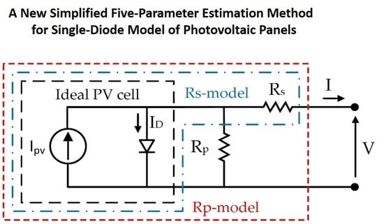
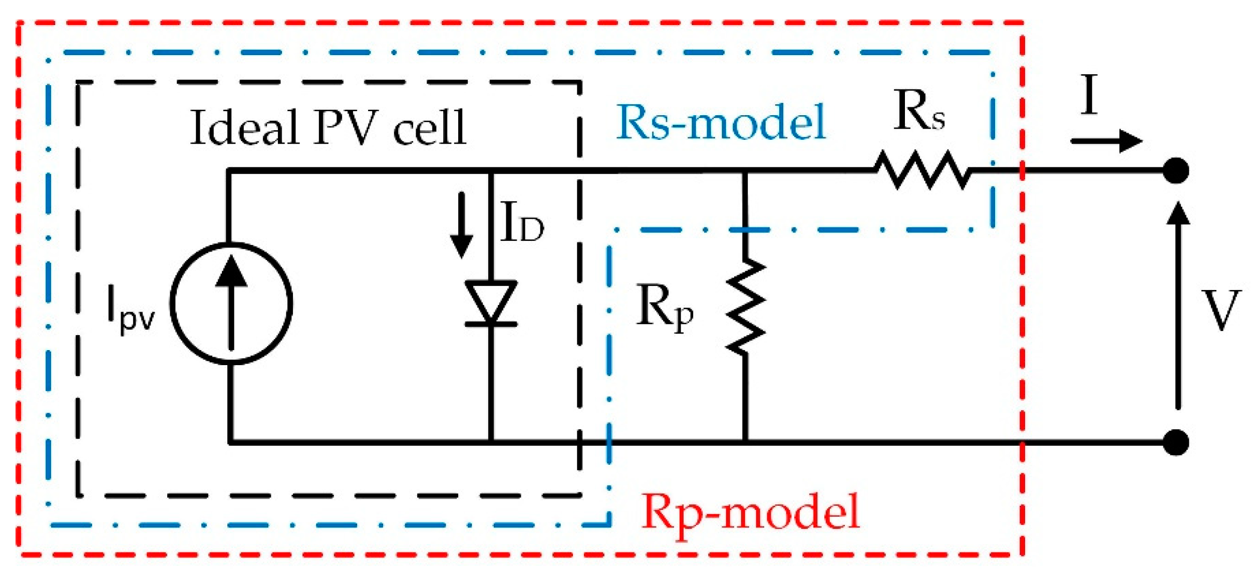
2. Single Diode Model of a PV Panel
- q is the electron charge (−1.60217646 × 10⁻¹⁹ C)
- A is the ideality factor of the diode
- k is the Boltzmann’s constant (−1.380653 × 10⁻²³ J/K)
- I0 represents the inverse saturation current
- T is the temperature (expressed in Kelvin)
3. State of the Art on Methods for Parameter Estimation
4. Proposed Five-Parameters Estimation Method
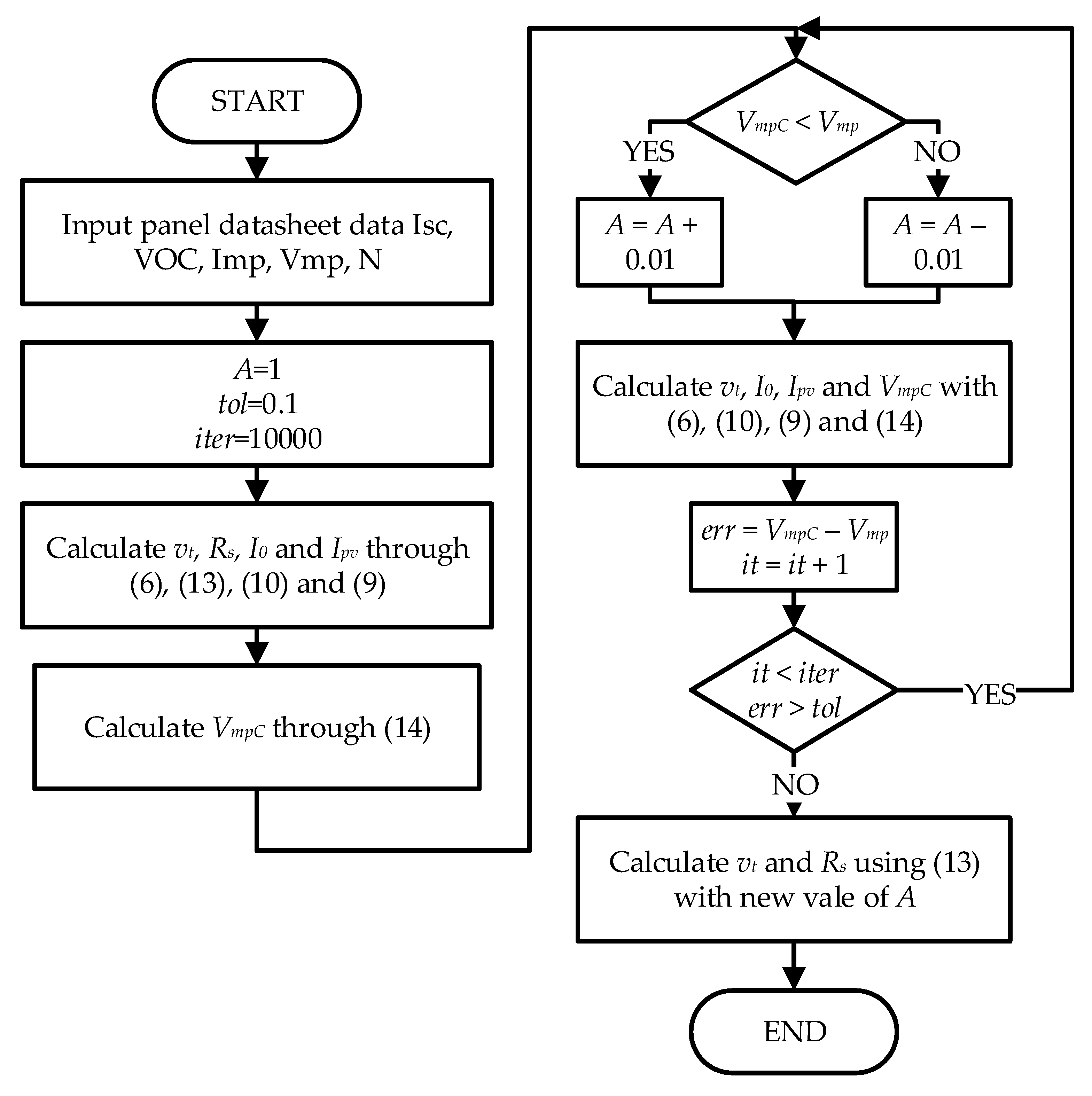
4.1. Step 1: Estimation of A and Rs Parameters
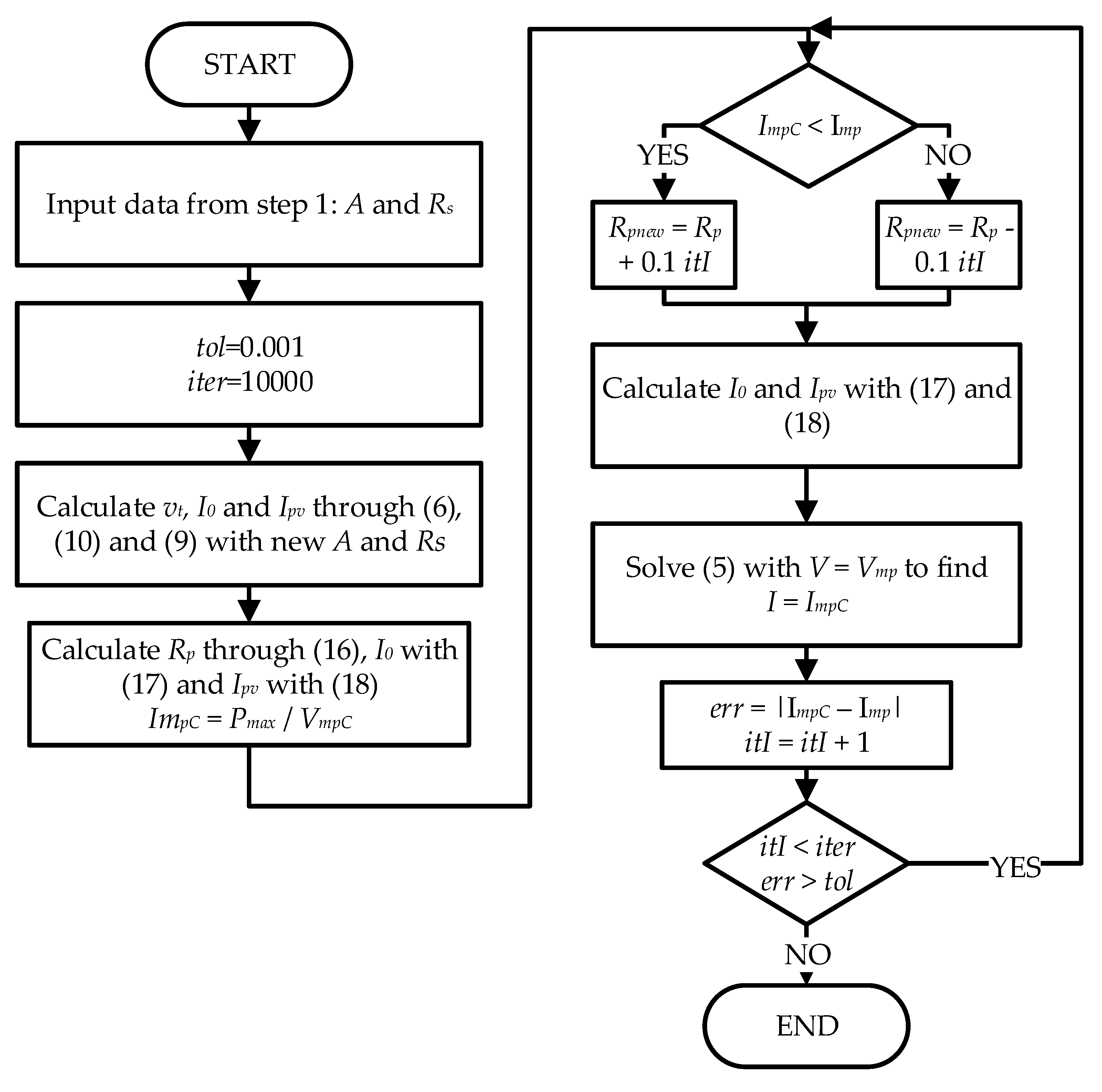
4.2. Step 2: Estimation of Rp Parameters
4.3. Electrical Variation Model and Error Metric
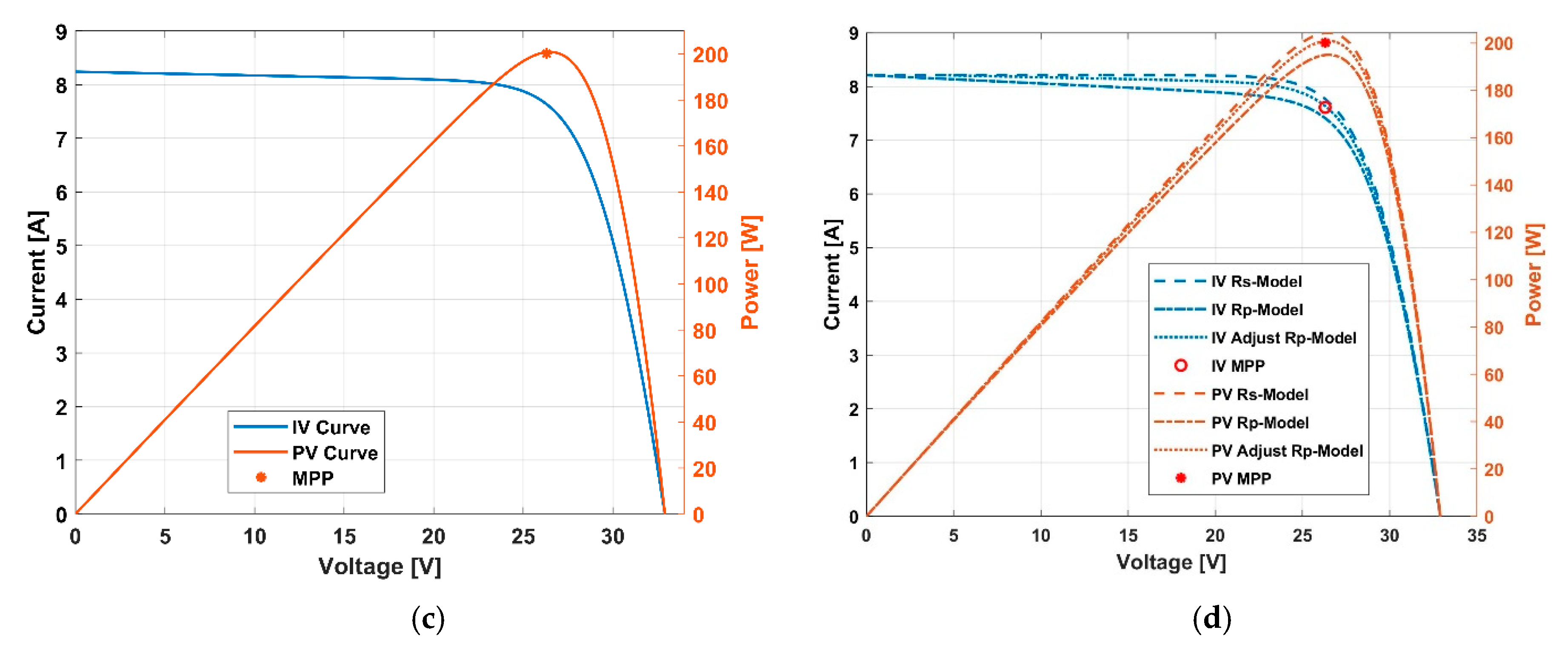
5. Results and discussion
6. Conclusions
Author Contributions
Funding
Conflicts of Interest
Nomenclature
| Label | Description (unit) | I0 | Diode Saturation current [A] |
| PV | Photovoltaic | Ipv | Photocurrent [A] |
| MPP | Maximum power point | vt | Thermal voltage [V] |
| MPPT | Maximum power point tracking | RMSE | Root mean square error current [A] |
| STC | Standard test condition | ||
| Isc | Short circuit current [A] | NRMSE | Normalized root mean square error current [%] |
| Isc,STC | Short circuit current at STC [A] | ||
| Voc | Open circuit voltage [V] | NRMSEAv | Average normalized root mean square error current [%] |
| VOC,STC | Open circuit voltage at STC [V] | ||
| Pmax | Maximum power [W] | q | Electron charge (−1.60217646 × 10⁻¹⁹) [C] |
| N | Number of cells in series [-] | ||
| Vmp | Maximum power point voltage [V] | k | Boltzmann’s costant (−1.380653 × 10⁻²³) [J/K] |
| Imp | Maximum power point current [A] | ||
| A | Diode ideality factor [-] | T | Temperature [°C] |
| Rs | Series resistance [Ω] | TSTC | Temperature at STC (25°C or 298.15K) [°C] |
| Rs,STC | Series resistance at STC [Ω] | ||
| Rp | Shunt resistance [Ω] | Kv | Temperature coefficient of open circuit voltage [V/°C] [%/°C] |
| Rp,STC | Shunt resistance at STC [Ω] | ||
| G | Solare irradiance [W/m2] | Ki | Temperature coefficient of short circuit current [A/°C] [%/°C] |
| GSTC | Solar irradiance at STC [W/m2] | ||
| kR | Linear temperature coefficient [-] | B | Exponential solar irradiance [-] |
Appendix A
| %Initial Data |
| q = 1.6*10^(−19); |
| k = 1.38*10^(−23); %Boltzmann’s costant |
| T = 298; %Temperature in Kelvin |
| %% Datasheet table STC value of KC200GT panel |
| Isc = 8.21 % Short circuit current |
| Voc = 32.9 %Open circuit voltage |
| Imp = 7.6 %Maximum power current |
| Vmp = 26.3 %Maximum power voltage |
| N = 54 %number of cells connected in series |
| Pmax = Vmp*Imp %Maximum power point |
| A = 1; |
| Vt = (k*A*T*N)/q; |
| Rs = (Voc/Imp) − (Vmp/Imp) + ((vt/Imp)*log((vt)/(vt + Vmp))); |
| I0 = Isc/(exp(Voc/vt) − exp(Rs*Isc/vt)); |
| Ipv = I0*((exp(Voc/vt)) − 1); |
| %% First step |
| iter = 10,000; |
| it = 0; |
| tol = 0.1; |
| A1 = A; |
| VmpC = (vt*(log((Ipv+I0-Imp)/I0))) − (Rs*Imp); |
| e1 = VmpC − Vmp; |
| Rs1 = Rs; |
| while (it < iter & e1 > tol) |
| if VmpC < Vmp |
| A1 = A1 − 0.01; |
| else |
| A1 = A1 + 0.01; |
| end |
| vt1 = (k*A1*T*N)/q; |
| I01 = Isc/(exp(Voc/vt1) − exp(Rs1*Isc/vt1)); |
| Ipv1 = I01*((exp(Voc/vt1)) − 1); |
| VmpC = (vt1*(log((Ipv1 + I01 − Imp)/I01))) − (Rs1*Imp); |
| e1 = (VmpC − Vmp); |
| it = it + 1; |
| end |
| vt1 = (k*A1*T*N)/q; |
| Rs1 = (Voc/Imp) − (VmpC/Imp) + ((vt1/Imp)*log((vt1)/(vt1 + VmpC))); |
| %% Second step |
| tolI = 0.001; |
| iter = 10000; |
| itI = 0; |
| I01 = Isc/(exp(Voc/vt1) − exp(Rs1*Isc/vt1)); |
| Ipv1 = I01*((exp(Voc/vt1))-1); |
| Rp = (( − Vmp)*(Vmp + (Rs1*Imp)))/(Pmax − (Vmp*Ipv1) + (Vmp*I01*(exp(((Vmp + (Rs1*Imp))/vt1) − 1)))); |
| %calculate I0 with new Rp value |
| I02 = (Isc*(1 + Rs1/Rp) − Voc/Rp)/(exp(Voc/vt1) − exp(Rs1*Isc/vt1)); |
| Ipv2 = I02*((exp(Voc/vt1)) − 1) + Voc/Rp; |
| ImpC = Pmax/VmpC; |
| Err = abs(Imp − ImpC); |
| Rpnew = Rp; |
| while err>tolI & itI<iter |
| if ImpC<Imp |
| Rpnew = Rp + 0.1*itI; |
| elseif ImpC>=Imp |
| Rpnew = Rp − 0.1*itI; |
| end |
| %Calculate I0 with Rpnew |
| I02 = (Isc*(1 + Rs1/Rpnew) − Voc/Rpnew)/(exp(Voc/vt1) − exp(Rs1*Isc/vt1)); |
| Ipv2 = I02*((exp(Voc/vt1)) − 1) + Voc/Rpnew; |
| eqn = @(ImpC) Ipv2 − (I02*(exp((Vmp + (Rs1*ImpC))/vt1) − 1)) − ImpC − (Vmp + Rs1*ImpC)/Rpnew; |
| current_c = Imp; |
| s = fzero(eqn,current_c); |
| ImpC = s; |
| itI = itI+1; |
| err = abs(Imp − ImpC); |
| end |
| X = sprintf(’A = %.2f, I0 = %d, Ipv = %.3f, Rs = %f, Rp = %f’, A1,I02,Ipv2,Rs1,Rpnew); |
| disp(X); |
References
- BNEF Global Trends in Renewable Energy Investment 2019. Available online: http://www.fs-unep-centre.org (accessed on 29 September 2019).
- Alaaeddin, M.; Sapuan, S.; Zuhri, M.; Zainudin, E.; AL- Oqla, F. Photovoltaic applications: Status and manufacturing prospects. Renew. Sustain. Energy Rev. 2019, 102, 318–332. [Google Scholar] [CrossRef]
- Dall’Anese, E.; Dhople, S.; Johnson, B.; Giannakis, G. Optimal Dispatch of Residential Photovoltaic Inverters under Forecasting Uncertainties. IEEE J. Photovolt. 2015, 5, 350–359. [Google Scholar] [CrossRef]
- Orsetti, C.; Muttillo, M.; Parente, F.; Pantoli, L.; Stornelli, V.; Ferri, G. Reliable and Inexpensive Solar Irradiance Measurement System Design. Procedia Eng. 2016, 168, 1767–1770. [Google Scholar] [CrossRef]
- Fusacchia, P.; Muttillo, M.; Leoni, A.; Pantoli, L.; Parente, F.; Stornelli, V.; Ferri, G. A Low Cost Fully Integrable in a Standard CMOS Technology Portable System for the Assessment of Wind Conditions. Procedia Eng. 2016, 168, 1024–1027. [Google Scholar] [CrossRef]
- De Rubeis, T.; Nardi, I.; Muttillo, M. Development of a low-cost temperature data monitoring. An upgrade for hot box apparatus. J. Phys. Conf. Ser. 2017, 923, 1. [Google Scholar] [CrossRef]
- Pantoli, L.; Paolucci, R.; Muttillo, M.; Fusacchia, P.; Leoni, A. A Multisensorial Thermal Anemometer System. Lect. Notes Electr. Eng. 2017, 431, 330–337. [Google Scholar] [CrossRef]
- Ferri, G.; Parente, F.; Stornelli, V.; Barile, G.; Pantoli, L. Automatic Bridge-Based Interface for Differential Capacitive Full Sensing. Procedia Eng. 2016, 168, 1585–1588. [Google Scholar] [CrossRef]
- Barile, G.; Ferri, G.; Parente, F.; Stornelli, V.; Depari, A.; Flammini, A.; Sisinni, E. A standard CMOS bridge-based analog interface for differential capacitive sensors. In Proceedings of the 13th Conference on Ph.D. Research in Microelectronics and Electronics (PRIME), Taormina, Italy, 12–15 June 2017. [Google Scholar]
- Lukač, N.; Žlaus, D.; Seme, S.; Žalik, B.; Štumberger, G. Rating of roofs’ surfaces regarding their solar potential and suitability for PV systems, based on LiDAR data. Appl. Energy 2013, 102, 803–812. [Google Scholar] [CrossRef]
- Nardi, I.; de Rubeis, T.; Taddei, M.; Ambrosini, D.; Sfarra, S. The energy efficiency challenge for a historical building undergone to seismic and energy refurbishment. Energy Procedia 2017, 133, 231–242. [Google Scholar] [CrossRef]
- Li, X.; Wen, H.; Hu, Y.; Jiang, L. A novel beta parameter based fuzzy-logic controller for photovoltaic MPPT application. Renew. Energy 2019, 130, 416–427. [Google Scholar] [CrossRef]
- Baka, M.; Manganiello, P.; Soudris, D.; Catthoor, F. A cost-benefit analysis for reconfigurable PV modules under shading. Sol. Energy 2019, 178, 69–78. [Google Scholar] [CrossRef]
- Orioli, A.; Di Gangi, A. A procedure to evaluate the seven parameters of the two-diode model for photovoltaic modules. Renew. Energy 2019, 139, 582–599. [Google Scholar] [CrossRef]
- Chin, V.; Salam, Z.; Ishaque, K. Cell modelling and model parameters estimation techniques for photovoltaic simulator application: A review. Appl. Energy 2015, 154, 500–519. [Google Scholar] [CrossRef]
- Adamo, F.; Attivissimo, F.; Di Nisio, A.; Lanzolla, A.; Spadavecchia, M. Parameters estimation for a model of photovoltaic panels. In Proceedings of the XIX IMEKO World Congress Fundamental and Applied Metrology, Lisbon, Portugal, 6–11 September 2009. [Google Scholar]
- Lo Brano, V.; Orioli, A.; Ciulla, G.; Di Gangi, A. An improved five-parameter model for photovoltaic modules. Sol. Energy Mater. Sol. Cells 2010, 94, 1358–1370. [Google Scholar] [CrossRef]
- ALQahtani, A. A simplified and accurate photovoltaic module parameters extraction approach using matlab. In Proceedings of the IEEE International Symposium on Industrial Electronics, Hangzhou, China, 28–31 May 2012. [Google Scholar]
- Siddiqui, M.; Arif, A.; Bilton, A.; Dubowsky, S.; Elshafei, M. An improved electric circuit model for photovoltaic modules based on sensitivity analysis. Sol. Energy 2013, 90, 29–42. [Google Scholar] [CrossRef]
- Orioli, A.; Di Gangi, A. A procedure to calculate the five-parameter model of crystalline silicon photovoltaic modules on the basis of the tabular performance data. Appl. Energy 2013, 102, 1160–1177. [Google Scholar] [CrossRef]
- Lineykin, S.; Averbukh, M.; Kuperman, A. An improved approach to extract the single-diode equivalent circuit parameters of a photovoltaic cell/panel. Renew. Sustain. Energy Rev. 2014, 30, 282–289. [Google Scholar] [CrossRef]
- Vergura, S. A Complete and Simplified Datasheet-Based Model of PV Cells in Variable Environmental Conditions for Circuit Simulation. Energies 2016, 9, 326. [Google Scholar] [CrossRef]
- Batzelis, E.; Papathanassiou, S. A Method for the Analytical Extraction of the Single-Diode PV Model Parameters. IEEE Trans. Sustain. Energy 2016, 7, 504–512. [Google Scholar] [CrossRef]
- Jordehi, A. Time varying acceleration coefficients particle swarm optimisation (TVACPSO): A new optimisation algorithm for estimating parameters of PV cells and modules. Energy Convers. Manag. 2016, 129, 262–274. [Google Scholar] [CrossRef]
- Chen, Z.; Wu, L.; Lin, P.; Wu, Y.; Cheng, S. Parameters identification of photovoltaic models using hybrid adaptive Nelder-Mead simplex algorithm based on eagle strategy. Appl. Energy 2016, 182, 47–57. [Google Scholar] [CrossRef]
- Cuce, E.; Cuce, P.; Karakas, I.; Bali, T. An accurate model for photovoltaic (PV) modules to determine electrical characteristics and thermodynamic performance parameters. Energy Convers. Manag. 2017, 146, 205–216. [Google Scholar] [CrossRef]
- Muhsen, D.; Ghazali, A.; Khatib, T.; Abed, I. A comparative study of evolutionary algorithms and adapting control parameters for estimating the parameters of a single-diode photovoltaic module’s model. Renew. Energy 2016, 96, 377–389. [Google Scholar] [CrossRef]
- Bastidas-Rodriguez, J.; Petrone, G.; Ramos-Paja, C.; Spagnuolo, G. A genetic algorithm for identifying the single diode model parameters of a photovoltaic panel. Math. Comput. Simul. 2017, 131, 38–54. [Google Scholar] [CrossRef]
- Oliva, D.; Abd El Aziz, M.; Ella Hassanien, A. Parameter estimation of photovoltaic cells using an improved chaotic whale optimization algorithm. Appl. Energy 2017, 200, 141–154. [Google Scholar] [CrossRef]
- Bana, S.; Saini, R. Identification of unknown parameters of a single diode photovoltaic model using particle swarm optimization with binary constraints. Renew. Energy 2017, 101, 1299–1310. [Google Scholar] [CrossRef]
- Kang, T.; Yao, J.; Jin, M.; Yang, S.; Duong, T. A Novel Improved Cuckoo Search Algorithm for Parameter Estimation of Photovoltaic (PV) Models. Energies 2018, 11, 1060. [Google Scholar] [CrossRef]
- Chaibi, Y.; Salhi, M.; El-jouni, A.; Essadki, A. A new method to extract the equivalent circuit parameters of a photovoltaic panel. Sol. Energy 2018, 163, 376–386. [Google Scholar] [CrossRef]
- Şentürk, A. New method for computing single diode model parameters of photovoltaic modules. Renew. Energy 2018, 128, 30–36. [Google Scholar] [CrossRef]
- Yu, K.; Liang, J.; Qu, B.; Cheng, Z.; Wang, H. Multiple learning backtracking search algorithm for estimating parameters of photovoltaic models. Appl. Energy 2018, 226, 408–422. [Google Scholar] [CrossRef]
- Drouiche, I.; Harrouni, S.; Arab, A. A new approach for modelling the aging PV module upon experimental I–V curves by combining translation method and five-parameters model. Electr. Power Syst. Res. 2018, 163, 231–241. [Google Scholar] [CrossRef]
- Louzazni, M.; Khouya, A.; Amechnoue, K.; Gandelli, A.; Mussetta, M.; Crăciunescu, A. Metaheuristic Algorithm for Photovoltaic Parameters: Comparative Study and Prediction with a Firefly Algorithm. Appl. Sci. 2018, 8, 339. [Google Scholar] [CrossRef]
- Ayang, A.; Wamkeue, R.; Ouhrouche, M.; Djongyang, N.; Essiane Salomé, N.; Pombe, J.; Ekemb, G. Maximum likelihood parameters estimation of single-diode model of photovoltaic generator. Renew. Energy 2019, 130, 111–121. [Google Scholar] [CrossRef]
- De Blas, M.; Torres, J.; Prieto, E.; García, A. Selecting a suitable model for characterizing photovoltaic devices. Renew. Energy 2002, 25, 371–380. [Google Scholar] [CrossRef]
- Sera, D.; Teodorescu, R.; Rodriguez, P. PV panel model based on datasheet values. In Proceedings of the IEEE International Symposium on Industrial Electronics, Vigo, Spain, 4–7 June 2007. [Google Scholar]
- Villalva, M.; Gazoli, J.; Filho, E. Comprehensive Approach to Modeling and Simulation of Photovoltaic Arrays. IEEE Trans. Power Electron. 2009, 24, 1198–1208. [Google Scholar] [CrossRef]
- Mahmoud, Y.; Xiao, W.; Zeineldin, H. A Parameterization Approach for Enhancing PV Model Accuracy. IEEE Trans. Ind. Electron. 2013, 60, 5708–5716. [Google Scholar] [CrossRef]
- Tan, R.; Tai, P.; Mok, V. Solar irradiance estimation based on photovoltaic module short circuit current measurement. In Proceedings of the IEEE International Conference on Smart Instrumentation, Measurement and Applications (ICSIMA), Kuala Lumpur, Malaysia, 25–27 November 2013. [Google Scholar]
- Nayak, B.; Mohapatra, A.; Mohanty, K. Parameters estimation of photovoltaic module using nonlinear least square algorithm: A comparative study. In Proceedings of the Annual IEEE India Conference (INDICON), Mumbai, India, 13–15 December 2013. [Google Scholar]
- Accarino, J.; Petrone, G.; Ramos-Paja, C.; Spagnuolo, G. Symbolic algebra for the calculation of the series and parallel resistances in PV module model. In Proceedings of the International Conference on Clean Electrical Power (ICCEP), Alghero, Italy, 11–13 June 2013. [Google Scholar]
- Peng, L.; Sun, Y.; Meng, Z. An improved model and parameters extraction for photovoltaic cells using only three state points at standard test condition. J. Power Sources 2014, 248, 621–631. [Google Scholar] [CrossRef]
- Ayodele, T.; Ogunjuyigbe, A.; Ekoh, E. Evaluation of numerical algorithms used in extracting the parameters of a single-diode photovoltaic model. Sustain. Energy Technol. Assess. 2016, 13, 51–59. [Google Scholar] [CrossRef]
- Silva, E.; Bradaschia, F.; Cavalcanti, M.; Nascimento, A. Parameter Estimation Method to Improve the Accuracy of Photovoltaic Electrical Model. IEEE J. Photovolt. 2016, 6, 278–285. [Google Scholar] [CrossRef]
- Hejri, M.; Mokhtari, H. On the Comprehensive Parametrization of the Photovoltaic (PV) Cells and Modules. IEEE J. Photovolt. 2017, 7, 250–258. [Google Scholar] [CrossRef]
- Murtaza, A.; Munir, U.; Chiaberge, M.; Di Leo, P.; Spertino, F. Variable Parameters for a Single Exponential Model of Photovoltaic Modules in Crystalline-Silicon. Energies 2018, 11, 2138. [Google Scholar] [CrossRef]
- Tossa, A.; Soro, Y.; Azoumah, Y.; Yamegueu, D. A new approach to estimate the performance and energy productivity of photovoltaic modules in real operating conditions. Sol. Energy 2014, 110, 543–560. [Google Scholar] [CrossRef]
- Abdelhamid, H.; Edris, A.; Helmy, A.; Ismail, Y. Fast and accurate PV model for SPICE simulation. J. Comput. Electron. 2011, 18, 260–270. [Google Scholar] [CrossRef]
- Ishaque, K.; Salam, Z.; Taheri, H. Simple, fast and accurate two-diode model for photovoltaic modules. Sol. Energy Mater. Sol. Cells 2011, 95, 586–594. [Google Scholar]
- Diehl, W.; Sittinger, V.; Szyszka, B. Thin film solar cell technology in Germany. Surf. Coat. Technol. 2005, 193, 329–334. [Google Scholar] [CrossRef]
- Yamamoto, K.; Nakajima, A.; Yoshimi, M.; Sawada, T.; Fukuda, S.; Suezaki, T.; Ichikawa, M.; Koi, Y.; Goto, M.; Miguro, T.; et al. Thin film silicon solar cell and module. In Proceedings of the Conference Record of the Thirty-First IEEE Photovoltaic Specialists Conference, Lake Buena Vista, FL, USA, 3–7 January 2005. [Google Scholar]
- Khanna, V.; Das, B.; Bisht, D.; Vandana; Singh, P. A three diode model for industrial solar cells and estimation of solar cell parameters using PSO algorithm. Renewable Energy 2015, 78, 105–113. [Google Scholar] [CrossRef]
- Carrero, C.; Amador, J.; Arnaltes, S. A single procedure for helping PV designers to select silicon PV modules and evaluate the loss resistances. Renew. Energy 2007, 32, 2579–2589. [Google Scholar] [CrossRef]
- Rhouma, M.; Gastli, A.; Ben Brahim, L.; Touati, F.; Benammar, M. A simple method for extracting the parameters of the PV cell single-diode model. Renew. Energy 2017, 113, 885–894. [Google Scholar] [CrossRef]
- Root of nonlinear function—MATLAB fzero- MathWorks Italia. Available online: https://it.mathworks.com/help/matlab/ref/fzero.html (accessed on 29 September 2019).
- Tina, G.; Ventura, C. Evaluation and Validation of an Electrical Model of Photovoltaic Module Based on Manufacturer Measurement. Sustain. Energy Build. 2013, 22, 15–24. [Google Scholar]
- KC200GT—HIGH EFFICIENCY MULTICRYSTAL PHOTOVOLTAIC MODULE. Available online: https://www.kyocerasolar.com/dealers/product-center/archives/spec-sheets/KC200GT.pdf (accessed on 29 September 2019).
- WebPlotDigitizer—Copyright 2010–2019 Ankit Rohatgi. Available online: https://apps.automeris.io/wpd/ (accessed on 29 September 2019).


| Parameter | Value |
|---|---|
| ISC [A] | 8.21 |
| VOC [V] | 32.9 |
| Vmp [V] | 26.3 |
| Imp [A] | 7.61 |
| N | 54 |
| Kv [V/°C] | −0.123 |
| Ki [A/°C] | 0.0318 |
| Methods | Parameters | Error | |||||
|---|---|---|---|---|---|---|---|
| A | I0 [nA] | Ipv | Rs [mΩ] | Rp [Ω] | RMSE [A] | NRMSE [%] | |
| Villalva | 1.3 | 85.2 | 8.193 | 138.7 | 466 | 0.23 | 3.02 |
| Nayak | 1.241 | 35.8 | 8.193 | 198.4 | 599.9 | 0.15 | 1.96 |
| Mahmoud | 1.412 | 367 | 8.193 | 131.4 | ∞ | 0.21 | 2.79 |
| Accarino | 1.079 | 2 | 8.193 | 236.3 | 204 | 0.11 | 1.49 |
| Silva | 1 | 0.3 | 8.193 | 271 | 171.2 | 0.19 | 2.54 |
| Hejri | 1.34 | 171 | 8.21 | 220 | 951.93 | 0.15 | 2.02 |
| Hejri 1 | 1.34 | 150 | 8.16 | 180 | 951.9 | 0.11 | 1.51 |
| Proposed 2 | 1.12 | 5.14 | 8.22 | 265.6 | 144.9 | 0.12 | 1.53 |
| Proposed | 1.1 | 3.27 | 8.196 | 218.5 | 164.2 | 0.07 | 0.87 |
| Methods | NRMSE [%] | NRMSE Av [%] | |||||
|---|---|---|---|---|---|---|---|
| Condition | |||||||
| Solar irradiance [W/m2] | Temperature [°C] | ||||||
| 800 | 600 | 400 | 200 | 50 | 75 | ||
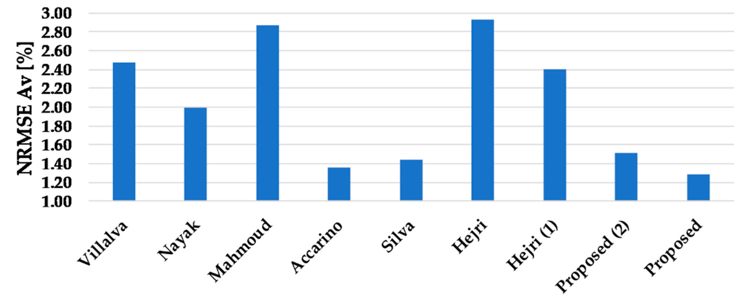
| Villalva | 1.9 | 2.23 | 1.98 | 2.99 | 1.94 | 2.99 | 2.44 |
| Nayak | 1.45 | 2.13 | 2.07 | 2.71 | 0.99 | 1.86 | 1.88 |
| Mahmoud | 1.58 | 2.2 | 2.6 | 4.76 | 1.52 | 2.38 | 2.55 |
| Accarino | 1.62 | 2.66 | 3.35 | 4.26 | 0.94 | 2.04 | 2.34 |
| Silva | 1.57 | 2.96 | 4.25 | 5.88 | 0.69 | 1.76 | 2.81 |
| Hejri | 1.51 | 2.12 | 2.33 | 3.84 | 1.37 | 1.2 | 2.06 |
| Hejri 1 | 1.33 | 2.03 | 2.16 | 3.7 | 0.99 | 1.64 | 1.91 |
| Proposed 2 | 0.73 | 1.61 | 2.09 | 2.94 | 0.93 | 0.93 | 1.54 |
| Proposed | 1.62 | 2.53 | 3.05 | 3.73 | 1.14 | 2.28 | 2.17 |
| Methods | NRMSE [%] | NRMSE Av [%] | |||||
|---|---|---|---|---|---|---|---|
| Condition | |||||||
| Solar irradiance [W/m2] | Temperature [°C] | ||||||
| 800 | 600 | 400 | 200 | 50 | 75 | ||
| Villalva | 1.47 | 1.88 | 2.21 | 4.12 | 1.85 | 2.78 | 2.48 |
| Nayak | 1.26 | 2.01 | 2.37 | 3.86 | 0.92 | 1.61 | 2.00 |
| Mahmoud | 1.44 | 2.43 | 3.56 | 6.25 | 1.45 | 2.2 | 2.87 |
| Accarino | 0.97 | 1.48 | 1.21 | 1.82 | 0.81 | 1.71 | 1.36 |
| Silva | 0.86 | 1.39 | 1.28 | 2.07 | 0.6 | 1.39 | 1.45 |
| Hejri | 2.13 | 3.16 | 4.16 | 6.26 | 1.49 | 1.28 | 2.93 |
| Hejri 1 | 1.45 | 2.48 | 3.41 | 5.59 | 0.97 | 1.45 | 2.41 |
| Proposed 2 | 1.3 | 1.76 | 1.74 | 2.39 | 1.08 | 0.84 | 1.52 |
| Proposed | 0.92 | 1.38 | 1.09 | 1.75 | 1.01 | 1.95 | 1.28 |
© 2019 by the authors. Licensee MDPI, Basel, Switzerland. This article is an open access article distributed under the terms and conditions of the Creative Commons Attribution (CC BY) license (http://creativecommons.org/licenses/by/4.0/).
Share and Cite
Stornelli, V.; Muttillo, M.; de Rubeis, T.; Nardi, I. A New Simplified Five-Parameter Estimation Method for Single-Diode Model of Photovoltaic Panels. Energies 2019, 12, 4271. https://doi.org/10.3390/en12224271
Stornelli V, Muttillo M, de Rubeis T, Nardi I. A New Simplified Five-Parameter Estimation Method for Single-Diode Model of Photovoltaic Panels. Energies. 2019; 12(22):4271. https://doi.org/10.3390/en12224271
Chicago/Turabian StyleStornelli, Vincenzo, Mirco Muttillo, Tullio de Rubeis, and Iole Nardi. 2019. "A New Simplified Five-Parameter Estimation Method for Single-Diode Model of Photovoltaic Panels" Energies 12, no. 22: 4271. https://doi.org/10.3390/en12224271
APA StyleStornelli, V., Muttillo, M., de Rubeis, T., & Nardi, I. (2019). A New Simplified Five-Parameter Estimation Method for Single-Diode Model of Photovoltaic Panels. Energies, 12(22), 4271. https://doi.org/10.3390/en12224271