Article

Luenberger-Sliding Mode Observer Based Backstepping Control for the SCR System in a Diesel Engine

1
School of Advanced Manufacturing, Chongqing University of Posts and Telecommunications, Chongqing 400065, China
2
School of Automation, Chongqing University of Posts and Telecommunications, Chongqing 400065, China
*
Author to whom correspondence should be addressed.
Energies 2019, 12(22), 4270; https://doi.org/10.3390/en12224270
Submission received: 25 October 2019 / Revised: 4 November 2019 / Accepted: 7 November 2019 / Published: 8 November 2019
(This article belongs to the Section B: Energy and Environment)

Abstract

:
In order to keep the ammonia (NH3) slip of the downstream selective catalytic reduction (SCR) system at a low level and simultaneously achieve a high nitrogen oxide (NOX) conversion rate, a Luenberger-sliding mode observer based backstepping control method is proposed. Considering that the internal working condition of the catalyst cannot be measured by commercial sensors directly, a Luenberger-sliding mode observer is designed to estimate the ammonia concentration at the middle of the catalyst. In addition, based on the stepped distributed characteristic of the surface ammonia coverage ratio along the SCR axial direction, a backstepping control method is utilized for the SCR system, in which the SCR system is decomposed into two subsystems. Firstly, the Lyapunov function is designed to ensure the convergence of the downstream subsystem, and then the virtual control law is obtained. After that, taking the virtual control law as the tracking target of the upstream subsystem, the Lyapunov function of virtual control law is given. Finally, the actual control law of the whole closed loop system is acquired. Simulations under different conditions are conducted to investigate the effect of the proposed control method. In addition, comparisons with the traditional PID (Proportion Integration Differentiation) control are presented. Results show that the proposed method is much better than the PID control method in overshoot, setting time, and tracking error.

Graphical Abstract

1. Introduction

Diesel engines have attracted more and more attention in recent years due to their high economy, high power, and low CO and HC emissions [1,2,3]. However, owing to the special combustion process, a diesel engine produces much more nitrogen oxide (NOX) and particulate matter (PM), which is harmful to the environment and human health. Various regulations have been legislated against diesel engine NOX and PM emissions. In order to meet stringent regulations, devices such as selective catalytic reduction (SCR) systems and diesel particle filters (DPF) are installed in post-processing systems to reduce emissions. SCR refers to the use of reducing agents to selectively react with NOx in flue gas and generate non-toxic and pollution-free N2 and H2O under the action of a catalyst. Generally, in SCR systems, 32.5% of aqueous urea solution is injected into the tail gas pipe of the engine; urea is then decomposed into ammonia, which reacts with NOx to generate N2 and H2O. However, excessive urea can lead to NH3 leakage in the tailpipe and increase the usage cost. On the other hand, insufficient NH3 injection will lead to low NOx conversion and higher tail pipe NOx emissions [3,4]. A great deal of research has been done to minimize NOx emissions and limit NH3 leaks at the same time, in which a promising method is to control the NH3 concentration and coverage of NH3 in the SCR catalyst at the optimum [5]. NH3 coverage and the ammonia coverage ratio are defined in (1), where Θ is NH3 storage capacity and M N H 3 is the amount of NH3 stored inside the SCR catalyst.
θ N H 3 = M N H 3 Θ
Much research has been conducted into SCR control systems [4,5,6]. In general, the SCR control strategy can be divided into non-model-based [7,8] and model-based [9,10,11,12,13,14,15,16,17]. The non-model-based methods include the pulse spectrum-based blue jet control method [7] and the PID control method [8]. Although the non-model-based method is relatively mature, its performance in transient and low temperature conditions makes it increasingly difficult to meet stricter emission regulations due to the problems of time delay, system inertia, and sensor measurement error and system uncertainty. As emission regulations become more and more stringent, model-based methods, such as predictive control [9], are needed urgently. Simulation and test bench results show that, compared to the non-model-based method, the model-based control method has higher accuracy and better environmental adaptability.
It should be mentioned that the values of NH3 concentration and NH3 coverage of the catalyst is vital for the SCR control system. Unfortunately, it is inconvenient to measure NH3 coverage directly through commercial sensors. To address the problem, observer based methods are prospective and widely used. Reference [18] presents an observer for estimating the NH3 concentration of catalysts in SCR. The observer can be used for NH3 distribution control of the SCR catalyst and fault diagnosis of the diesel engine. Experiments show that the observer estimates converge to the sensor readings and can track the values well. However, the concentration cannot be estimated well in the first 1100 seconds. In [4], an approach by utilizing two post-selective-catalytic-reduction nitrogen oxide sensors with different ammonia cross-sensitivity factors is proposed to estimate the nitrogen oxide concentration, the ammonia concentration, and the ammonia surface coverage ratio. Experimental results show that the proposed method can be useful in reducing the cost of SCR diagnosis, NH3 coverage estimation, and advanced SCR controls. In addition, an extended Kalman filter [19] can also be utilized to estimate the NOx sensor cross-sensitivity to ammonia. It is noteworthy that the performance of an urea-SCR system may be related to the NH3/NOX ratio and the NO/NO2 ratio. Studies show that the ratio of NO to NO2 varies with the reduction rate and conversion efficiency of NOX [1]. A sliding mode observer is widely used in system state estimation because of its strong robustness [20,21,22,23]. S. Hasan [24] introduced the Luenberger term into the design of the sliding mode observer, which not only improved the robustness of the observer, but also improved the speed of parameter estimation. Based on the above analysis, a Luenberger sliding mode observer is designed to estimate the state of the two-cell SCR catalyst.
Backstepping control is mainly used to deal with robust control systems with nonlinear and parametric uncertainties [25,26]. SCR is a typical nonlinear system with uncertain parameters, which is very suitable for backstepping control. Thus, in [27], the backstepping control is used successfully, but the unmeasurable problem of NH3 concentration is not mentioned.
In this paper, considering the advantages of the Luenberger-sliding mode observer [24] and backstepping control [25,26], a Luenberger-sliding mode observer based backstepping control method is applied to a nonlinear SCR system. The aims of this work are to simultaneously minimize the NOx emissions and limit the NH3 slip under a certain input and output constraint. A Luenberger-sliding mode observer is designed to estimate NH3 concentration and then, based on the Lyapunov stability analysis and the stepped distributed characteristic of the surface NH3 coverage ratio along the SCR axial direction, a backstepping control method is designed for SCR system adblue dosing. After that, the stability analysis of the proposed control strategy is described. The proposed approach is validated through computer simulations that are compared with the traditional PID control. Simulation results show that the system controlled by the proposed method has promising performance in overshoot, setting time, and tracking error.

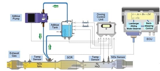
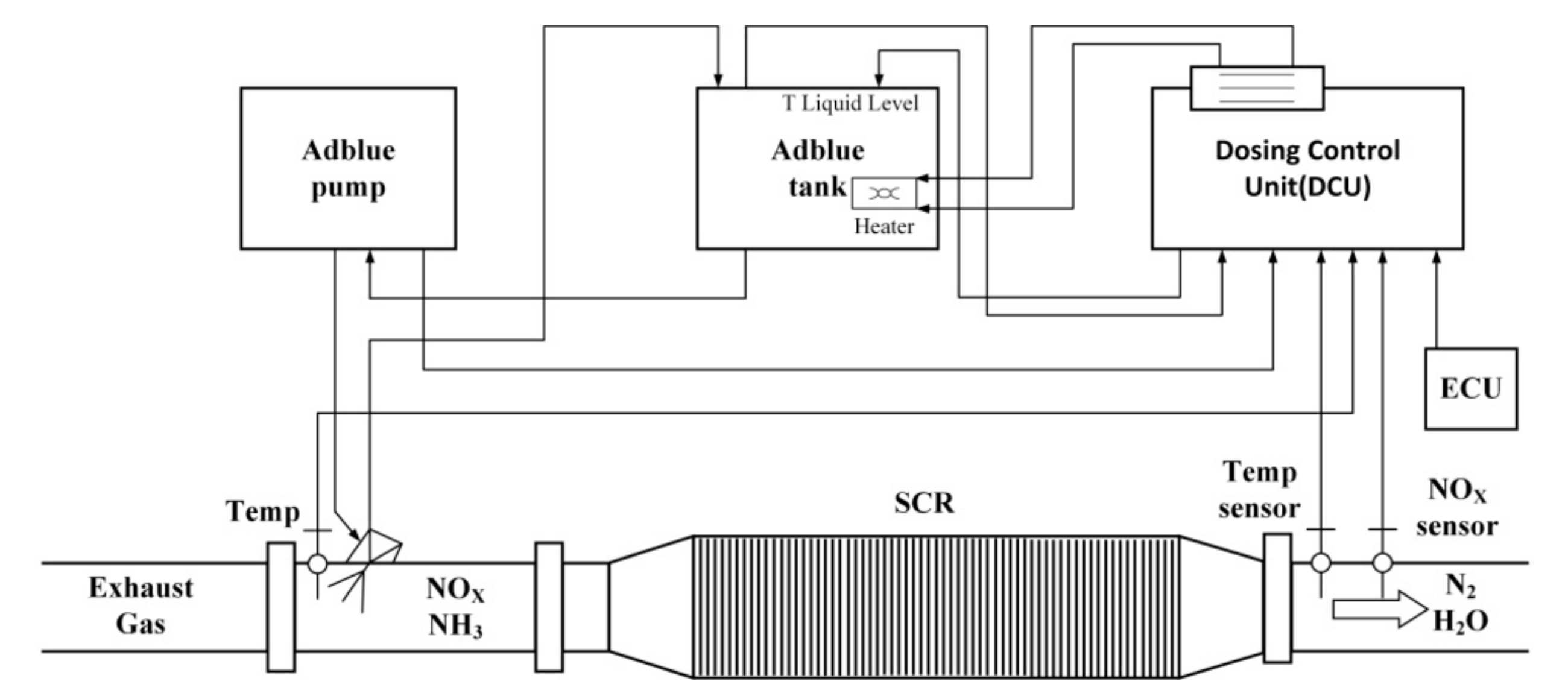
2. Selective Catalytic Reduction System

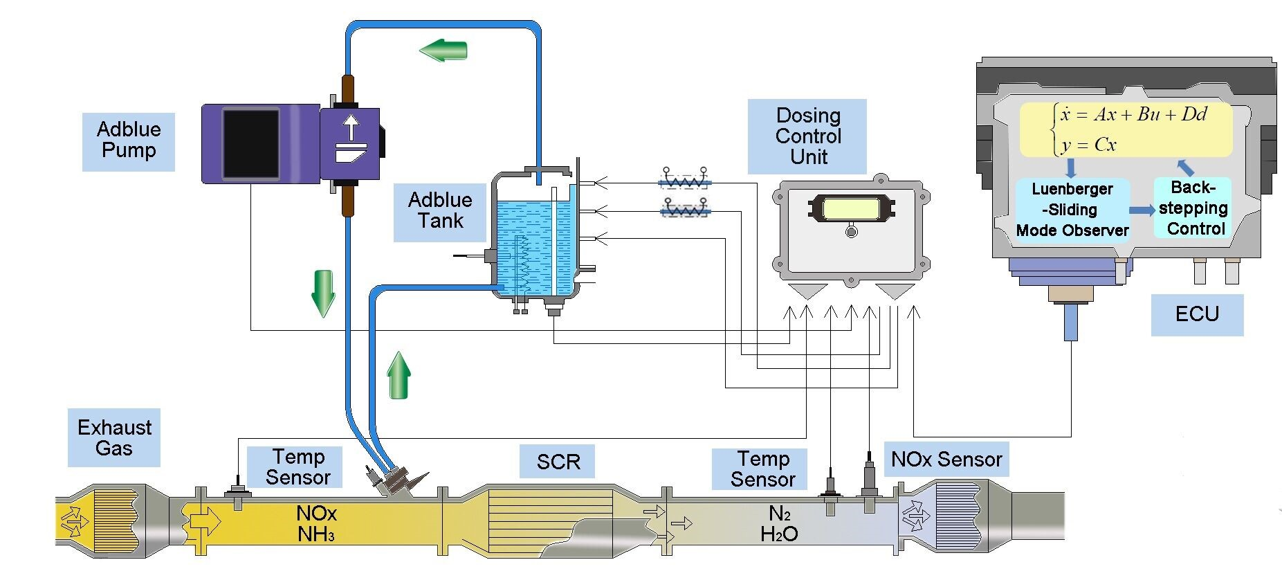
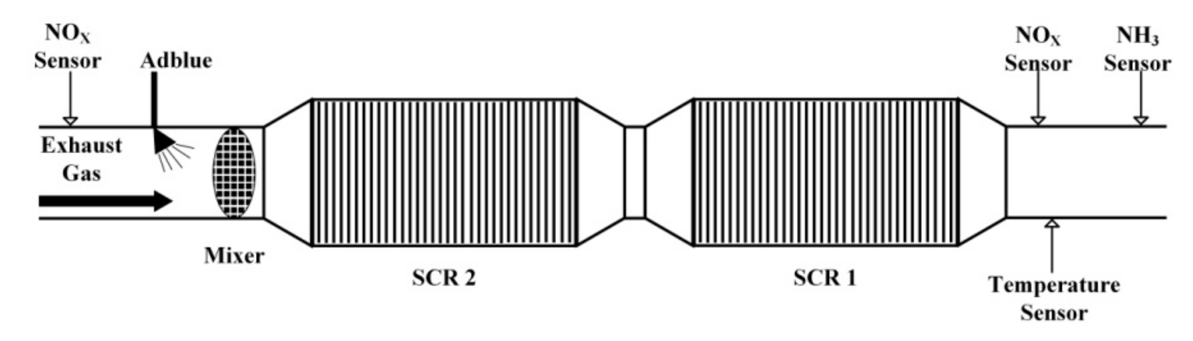
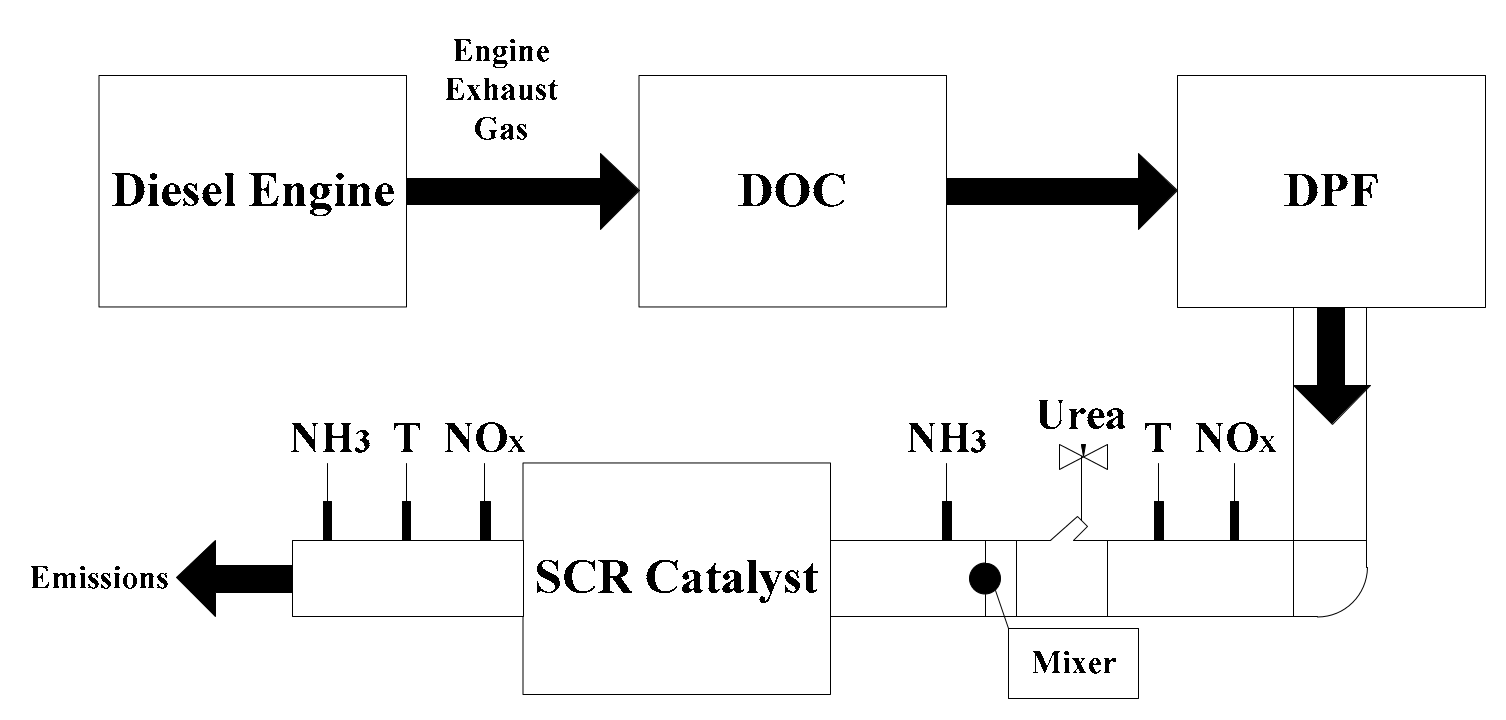
2.1. SCR System Operation Principles

Figure 1 is a schematic diagram of an SCR system, in which temperature, NOx, and NH3 sensors are located upstream and downstream of the SCR catalyst. In order to monitor the status of the intermediate catalyst, NOx and NH3 sensors are installed between two SCR batteries. Note that the inlet NOx measurement will not be contaminated by NH3, while the intermediate and downstream NOx sensors will be affected by the cross sensitivity of NH3. According to [27], the concentration of NOx is a combination of the NOx and NH3 concentrations, as shown in (2):
C N O x , m e a = C N O x + K C N H 3
where C N O x , m e a is the NOx sensor reading, C N O x is the true value of the NOx concentration, C N H 3 is the NH3 concentration, and K denotes the cross-sensitivity factor. In this paper, K is considered to be a constant.
The reduction involves three processes. First, the urea solution sprayed into the upstream exhaust pipe is converted into NH3, which generally consists of three chemical reactions: Urea solution evaporation, urea decomposition, and isocyanic acid hydrolysation. The main chemical reactions are summarized as:
Aqueous urea solution evaporation:
( N H 2 ) C O ( l i q u i d ) ( N H 2 ) 2 C O ( s o l i d ) + H 2 O .
Urea decomposition:
( N H 2 ) 2 C O 2 N H 3 + H N C O .
Isocyanic acid (HNCO) hydrolysation:
H N C O + H 2 O N H 3 + C O 2 .
Then, the converted NH3 is adsorbed on the surface of the catalyst matrix. Finally, the NH3 reacts with NOx to form nitrogen molecules.
It should be noted that that urea can be completely converted in the upstream tailpipe if the catalyst pool has a good geometric design and the exhaust has a suitable temperature [28]. Therefore, it is reasonable to assume that 100% of the urea aqueous solution is converted to gaseous NH3 before the SCR catalyst unit.
The NH3 adsorption and desorption reactions can be expressed as [29]:
Z + N H 3 Z N H 3
Z N H 3 Z + N H 3
where Z is the active substrate site of the SCR catalyst cell and Z N H 3 represents NH3 adsorbed on the SCR substrate. The adsorbed NH3 is active enough to reduce the NOx in terms of the chemical reactions. The main NOx reduction process can be summarized as follows:
4 N H 3 + 4 N O + O 2 4 N 2 + 6 H 2 O
4 N H 3 + 2 N O + 2 N O 2 4 N 2 + 6 H 2 O
8 N H 3 + 6 N O 2 7 N 2 + 12 H 2 O .
In some cases, when the gas temperature is quite high, the adsorbed NH3 can also be oxidized, as shown in (11):
4 N H 3 + 5 O 2 4 N O + 6 H 2 O .

2.2. SCR Dynamic Model and Analysis of Observability and Controllability

Assuming that the physical variables in the SCR catalyst unit are uniform, a SCR model is developed based on the above reaction. For convenience, the mass transfer and the surface phase concentration of species in the model are neglected. In this paper, the nonlinear model of the SCR model is expressed using the state-space form [29]:
C ˙ N O θ ˙ C ˙ N H 3 = C N O ( Θ r red θ + F V ) + r o x i Θ θ θ ( r ads C N H 3 + r d e s + r r e d C N O + r o x i ) + r a d s C N H 3 C N H 3 [ Θ r a d s ( 1 θ ) + F V ] + Θ r des θ + 0 0 F V C N H 3 , i n + F V 0 0 C N O , i n
where, C N O , C N H 3 , C N O , i n , and C N H 3 , i n are the concentrations of NO, NH3, inlet NO, and inlet NH3, respectively. r r e d , r a d s , r d e s , and r o x i are standard reaction rate, adsorption rate, desorption rate, and oxidation rate, respectively. F is the exhaust flow rate and V is the SCR volume. θ denotes the ammonia coverage ratio and R is the universal gas constant.
Let
x = [ x 1   x 2   x 3 ] T
where x 1 = C N O , x 2 = θ , x 3 = C N H 3 .
Linearize the nonlinear model with respect to operating points and obtain the linear state space equation:
x ˙ = A x + B u + D d y = C x
where
A = A 11 A 12 A 13 A 21 A 22 A 23 A 31 A 32 A 33 ,   B = 0 0 F V ,   D = F V 0 0 ,   C = 0 0 1 ,
A 11 = Θ r r e d x 2 F V ,   A 12 = Θ r r e d x 1 + Θ r o x i ,
A 13 = 0 ,   A 21 = r r e d x 2 ,   A 23 = r a d s ( 1 x 2 ) ,  
A 22 = r a d s x 3 + r d e s + r r e d x 1 + r o x i ,   A 31 = 0 ,  
A 32 = Θ r a d s x 3 + Θ r d e s , A 33 = Θ r a d s ( 1 x 2 ) F V , u = C N H 3 , i n is the inlet ammonia concentration, d = C N O , i n is the inlet NO concentration.
The controllability grammian matrix takes the form:
Q C = 0 0 1 0 A 23 A 33 A 12 A 23 ( A 22 A 23 + A 23 A 33 ) ( A 23 A 32 + A 2 33 ) .
In most cases, the rank of the controllability grammian matrix is equal to 3. However, it may lose rank under certain operations:
(1)
A 23 = 0 , r a n k ( Q C ) = 1 ; the NH3 coverage ratio and the NOX concentration are uncontrollable. At that point, the NH3 coverage ratio reaches 100%. However, it will not happen in practice.
(2)
A 12 = 0 , r a n k ( Q C ) = 2 ; the NOX is uncontrollable. In the meantime, r o x i > r r e d × C N O , the reasonable working temperature, is below 600 °C. Therefore, the loss of controllability due to this condition is not expected operationally.

3. Observer Design and Stability Analysis

3.1. Two-Cell SCR Catalyst Ammonia Concentration Observer Design

According to [8], ammonia storage in SCR catalysts varies along the axis of the catalysts. Moreover, the ammonia storage in the upstream and downstream of the SCR catalysts has a direct impact on the conversion of NOx and the emission of NH3 in the tail gas. In order to express the internal state of the SCR catalytic converter more accurately, a two-cell SCR catalytic converter system is designed, shown in Figure 2 [18].
Considering the NH3 concentration and NH3 coverage ratio, the dynamic model is presented as follows:
θ ˙ 1 = θ 1 ( r ads , 1 C N H 3 , 1 + r d e s , 1 + r r e d , 1 C N O , 1 + r o x i , 1 ) + r a d s , 1 C N H 3 , 1
θ ˙ 2 = θ 2 ( r ads , 2 C N H 3 , 2 + r d e s , 2 + r r e d , 2 C N O , 2 + r o x i , 2 ) + r a d s , 2 C N H 3 , 2
C ˙ N H 3 , 1 = C N H 3 , 1 [ Θ 1 r a d s , 1 ( 1 θ 1 ) + F 1 V 1 ] + Θ 1 r des , 1 θ 1 + F 1 V 1 C N H 3 , 2
C ˙ N H 3 , 2 = C N H 3 , 2 [ Θ 2 r a d s , 2 ( 1 θ 2 ) + F 2 V 2 ] + Θ 2 r des , 2 θ 2 + F 2 V 2 C N H 3 , i n .
To estimate the NH3 coverage ratio, a Luenberger-sliding mode observer is proposed to observe the NH3 coverage ratio of the upstream cell [20]:
C ^ ˙ N H 3 , 2 = C ^ N H 3 , 2 [ Θ 2 r a d s , 2 ( 1 θ ^ 2 ) + F 2 V 2 ] + Θ 2 r des , 2 θ ^ 2 + F 2 V 2 C N H 3 , i n + l 2 , 2 ( C N H 3 , 1 C ^ N H 3 , 2 ) + k 2 , 2 sgn ( C N H 3 , 1 C ^ N H 3 , 2 )
where
θ ^ ˙ 2 = θ ^ 2 ( r ads , 2 C ^ N H 3 , 2 + r d e s , 2 + r r e d , 2 C ^ N O , 2 + r o x i , 2 ) + r a d s , 2 C ^ N H 3 , 2 + l 1 , 2 ( C ^ N H 3 , 2 C ^ N H 3 , 1 ) + k 1 , 2 sgn ( C ^ N H 3 , 2 C ^ N H 3 , 1 )
θ ^ ˙ 1 = θ ^ 1 ( r ads , 1 C ^ N H 3 , 1 + r d e s , 1 + r r e d , 1 C N O , 1 + r o x i , 1 ) + r a d s , 1 C ^ N H 3 , 1
C ^ ˙ N H 3 , 1 = C ^ N H 3 , 1 [ Θ 1 r a d s , 1 ( 1 θ ^ 1 ) + F 1 V 1 ] + Θ 1 r des , 1 θ ^ 1 + F 1 V 1 C N H 3 , 2 + l 2 , 1 ( C N H 3 , 1 C ^ N H 3 , 1 ) + k 2 , 1 sgn ( C N H 3 , 1 C ^ N H 3 , 1 )
C ^ ˙ N O , 2 = C ^ N O , 2 ( Θ 2 r red , 2 θ ^ 2 + F 2 V 2 ) + r o x i , 2 Θ 2 θ ^ 2 + F 2 V 2 C N O , i n
k 1 , 2 , k 2 , 1 , k 2 , 2 > 0 , 0 θ ^ 2 , θ ^ 2 1 , 0 C ^ N H 3 , 1 < 1 , C ^ N H 3 , 2 C ^ N H 3 , max < 1 .

3.2. Observer Stability Analysis

As mentioned above, the NH3 coverage ratio is one of the important factors for the NH3 storage distribution control, and its estimation requires the NH3 concentration. The observability is demonstrated in the following [28]:

3.2.1. Convergence Analysis of θ ^ 1

First, select the Lyapunov function candidate as:
V θ 1 = 1 2 θ ˜ 1 2 .
Then, the differentiate (25), gives:
V ˙ θ 1 = θ ˜ 1 θ ˜ ˙ 1 = θ ˜ 1 2 ( r ads , 1 C ^ N H 3 , 1 + r d e s , 1 + r r e d , 1 C N O , 1 + r o x i , 1 ) .
It is apparent that V ˙ θ 1 0 , which means that θ ^ 1 converges to θ 1 within a finite period of time.

3.2.2. Convergence Analysis of C ^ N H 3 , 2

Convergence analysis of C ^ N H 3 , 2
C ˜ ˙ N H 3 , 1 = F 1 V 1 C ˜ N H 3 , 2 l 2 , 1 ( C ˜ N H 3 , 1 ) k 2 , 1 sgn ( C ˜ N H 3 , 1 )
since 0 C ˜ N H 3 , 2 C N H 3 , max , let k 2 , 1 > F 1 , max V 1 C N H 3 , max , then C ^ N H 3 , 2 can converges to C N H 3 , 2 in a finite period of time. Once the sliding mode is reached in the short term, there will be C ˜ ˙ N H 3 , 1 = C ˜ N H 3 , 1 = 0 . That means:
F 1 V 1 C ˜ N H 3 , 2 = k 2 , 1 sgn ( C ˜ N H 3 , 1 )
sgn ( C ˜ N H 3 , 2 ) = sgn ( C ˜ N H 3 , 1 ) .
Select the Lyapunov function candidate as:
V C N H 3 , 2 = 1 2 C ˜ N H 3 , 2 2 .
Then, differentiate (31) gives:
V ˙ C N H 3 , 2 = C ˜ N H 3 , 2 C ˜ ˙ N H 3 , 2 = C ˜ N H 3 , 2 [ C ˜ N H 3 , 2 ( Θ 2 r a d s , 2 + F 2 V 2 ) + C N H 3 , 2 Θ 2 r a d s , 2 C ^ N H 3 , 2 Θ 2 r a d s , 2 θ ^ 2 + Θ 2 r a d s , 2 θ ˜ 2 l 2 , 2 ( C ˜ N H 3 , 2 ) k 2 , 2 sgn ( C ˜ N H 3 , 2 ) ] .
Let k 2 , 2 > max | C N H 3 , 2 Θ 2 r a d s , 2 C ^ N H 3 , 2 Θ 2 r a d s , 2 θ ^ 2 + Θ 2 r a d s , 2 θ ˜ 2 | ,then V ˙ C N H 3 , 2 is negative and definite, and C ^ N H 3 , 2 converges to C N H 3 , 2 in a finite period of time.

3.2.3. Convergence Analysis of θ ^ 2

Let C ˜ N H 3 , 2 = 0 as a sliding surface; once the sliding mode is reached, there will be C ˜ ˙ N H 3 , 2 = C ˜ N H 3 , 2 = 0 . Select the Lyapunov function candidate as:
V θ 2 = 1 2 θ ˜ 2 2 .
Then, differentiate (32) gives:
V ˙ θ 2 = θ ˜ 2 θ ˜ ˙ 2 = θ ˜ 2 [ θ ˜ 2 ( r d e s , 2 + r r e d , 2 C ^ N O , 2 + r o x i , 2 ) + θ ^ 2 r ads , 2 C ^ N H 3 , 2 θ ^ 2 r ads , 2 C ^ N H 3 , 2 + r ads , 2 C ˜ N H 3 , 2 l 1 , 2 ( C ˜ N H 3 , 2 ) k 1 , 2 sgn ( C ˜ N H 3 , 2 ] .
Let k 1 , 2 > | C N H 3 , 2 r a d s , 2 | max , then V ˙ θ 2 is negative and definite, and θ ^ 2 can converge to θ 2 in a finite period of time.

4. Backstepping Control Law Design

In order to keep NH3 leakage of the downstream SCR system at a low level and achieve a high NOx conversion rate at the same time, the controller should keep downstream NH3 coverage below constraint θ 1 * and control upstream NH3 coverage at the desired target, θ 2 * . Based on the two-cell SCR system model, the dynamic equations are expressed as [18]:
x ˙ 1 = F 1 ( x 1 , x 3 , T , C N O ) + G 1 ( x 1 , x 3 , T , C N O ) x 3
x ˙ 2 = F 2 ( x 1 , x 2 , Θ , T , F , V ) + G 2 ( x 1 , x 2 , Θ , T , F , V ) x 4
x ˙ 3 = F 3 ( x 4 , x 3 , Θ , T , F , V ) + G 3 ( x 4 , x 3 , Θ , T , F , V ) u
x ˙ 4 = F 4 ( x 3 , x 4 , T , C N O ) + G 4 ( x 3 , x 4 , T , C N O ) x 4
where
[ x 1   x 2   x 3   x 4 ] T = [ θ 1   C N H 3 , 1   θ 2   C N H 3 , 2 ] T
[ x 1 , min   x 2 , min   x 3 , min   x 4 , min ] T [ x 1   x 2   x 3   x 4 ] T [ x 1 , max   x 2 , max   x 3 , max   x 4 , max ] T
G 1 ( ) > 0 , G 2 ( ) > 0 , G 3 ( ) > 0 , G 4 ( ) > 0 , F 1 ( ) < 0 , F 4 ( ) < 0 .
According to the backstepping theory, the control law is designed to let x 4 approach θ 2 * under the condition x 1 θ 1 * .
u = G 2 ( x 2 ξ 1 ) G 4 ( x 4 θ 2 * ) K 3 s i g n ( x 3 ξ 2 ) F 3 + ξ ˙ 2 G 3
ξ 1 = K 1 x 1 θ 1 * 1 x 1
ξ 2 = K 2 x 2 ξ 1 F 2 + ξ ˙ 2 K 0 G 1 x 1 θ 1 * G 2
K 1 = C 2 G 4 ( 1 θ 1 * ) ( s i g n ( ( x 1 θ 1 * ) ( x 4 θ 2 * ) ) + 1 ) , C > 0
K 2 > F 2 max + K 0 G 1 , max x 2 , min
K 3 > G 4 , max x 4 θ 2 * max
s i g n ( x ) = 1 , x < 0 0 , x = 0 1 , x > 0
Stability of the backstepping is necessary for the controller design. For this system, two cases should be considered. One is x 1 > θ 1 * ; at this time, the downstream ammonia coverage ratio is fairly high, and x 1 can converge to θ 1 * . Another is x 1 θ 1 * ; the constraint is satisfied, and x 4 can converge to θ 2 * .

4.1. Stability Analysis of Case 1

(1) For Equation (34), the Lyapunov function candidate can be defined as:
V 1 = K 0 2 x ^ 1 2 > 0
where x ^ = x 1 θ 1 * and K 0 > 0 , and taking the time derivative of V 1 gives
V ˙ 1 = K 0 x ^ 1 x ^ ˙ 1 = K 0 x ^ 1 F 1 + K 0 x ^ 1 G 1 x 3 .
Combining (34) with (38) obtains:
V ˙ 1 = K 0 x ^ 1 ( x ^ 1 + θ 1 * ) ( r d e s , 1 + r r e d , 1 C N O , 1 + r o x i , i ) + K 0 r a d s , 1 x ^ 1 x 2 ( 1 ( x ^ 1 + θ 1 * ) ) K 0 x ^ 1 F 1 .
Select the virtual control input x 2 as ξ 1 . Combined, (40) and (43), gives
x 2 , v i r = ξ 1 = K 1 x 1 θ 1 * 1 x 1 = C ( x 1 θ 1 * ) 2 G 4 ( 1 θ 1 * ) ( 1 x 1 ) ( s i g n ( ( x 1 θ 1 * ) ( x 4 θ 2 * ) ) + 1 ) .
Then
V ˙ 1 = K 0 x ^ 1 ( x ^ 1 + θ 1 * ) ( r d e s , 1 + r r e d , 1 C N O , 1 + r o x i , i ) C K 0 x ^ 1 2 r a d s , 1 2 G 4 ( 1 θ 1 * ) ( s i g n ( ( x 1 θ 1 * ) ( x 4 θ 2 * ) ) + 1 )
bacause x ^ 1 > 0
x ^ 1 ( x ^ 1 + θ 1 * ) ( r d e s , 1 + r r e d , 1 C N O , 1 + r o x i , i ) > x ^ 1 2 ( r d e s , 1 + r r e d , 1 C N O , 1 + r o x i , i ) > 0
and
C K 0 x ^ 1 2 r a d s , 1 2 G 4 ( 1 θ 1 * ) ( s i g n ( ( x 1 θ 1 * ) ( x 4 θ 2 * ) ) + 1 ) 0
V ˙ 1 K 0 x ^ 1 ( x ^ 1 + θ 1 * ) ( r d e s , 1 + r r e d , 1 C N O , 1 + r o x i , i ) K 0 x ^ 1 2 ( x ^ 1 + θ 1 * ) ( r d e s , 1 + r r e d , 1 C N O , 1 + r o x i , i ) = Q 1 < 0
where, Q 1 is positive and definite. Therefore, x 1 can converge to θ 1 * .
(2) For Equation (35), in order to ensure that the real x 2 can converge to the desired value, x 2 , t a r , with the action of ξ 2 , the Lyapunov function candidate can be defined as:
V 2 = V 1 + 1 2 z 2 2 = K 0 2 x ^ 1 2 + 1 2 z 2 2
where
z 2 = x 2 ξ 1 .
Taking the time derivative of V 2 gives:
V ˙ 2 = K 0 x ^ 1 x ^ ˙ 1 + z 2 z ˙ 2 .
Because x 2 = ξ 1 + z 2 , according to (48) and (64), we can get:
V ˙ 2 K 0 x ^ 1 2 ( x ^ 1 + θ 1 * ) ( r d e s , 1 + r r e d , 1 C N O , 1 + r o x i , i ) + K 0 x ^ 1 G 1 z 2 + z 2 ( x ˙ 2 ξ ˙ 1 ) = Q 1 + z 2 ( K 0 x ^ 1 G 1 + F 2 + G 2 x 3 ξ ˙ 1 ) .
Letting x 3 = ξ 2 , as the virtual control signal, gets:
V ˙ 2 K 0 x ^ 1 2 ( x ^ 1 + θ 1 * ) ( r d e s , 1 + r r e d , 1 C N O , 1 + r o x i , i ) K 2 x 2 2 = Q 2 < 0
where, Q 2 is positive and definite. Therefore, x 2 can converge to x 2 , t a r .
(3) For Equation (36), in order to ensure that x 3 can converge to the desired value, x 3 , t a r , with the action of input signal u , the Lyapunov function candidate can be defined as:
V 3 = V 2 + 1 2 z 3 2
where z 3 = x 3 ξ 2 . Analogously, according to (59), taking the time derivative of V 3 gives:
V ˙ 3 = V ˙ 2 + z 3 z ˙ 3 Q 2 + G 2 z 2 z 3 + z 3 ( x ˙ 3 ξ ˙ 2 ) = Q 2 + z 3 ( G 2 z 2 + F 3 + G 3 u ξ ˙ 2 ) .
Based on (40) and (61), it can be achieved by:
V ˙ 3 Q 2 z 3 ( K 3 s i g n ( z 3 ) + g 4 ( x 4 θ 2 * ) ) = Q 3 .
Because K 3 > g 4 , max x 4 θ 2 * max , V ˙ 3 < 0 , x 3 can converge to x 3 , t a r .
According to the above mentioned analysis, based on the Lyapunov functions (47), (55), (60), and the control law (39), x 1 , x 2 , and x 3 can converge to the desired value, respectively.

4.2. Stability Analysis of Case 2

In this case, the NH3 coverage ratio of the downstream SCR system should be lower than the value x 2 , t a r , therefore, the Lyapunov function is design to prove that x 4 can converge to θ 2 * with the action of ξ 2 .
(1) For Equation (34), select ξ 2 as the virtual control input of x 3 ; the Lyapunov function candidate can be defined as:
V 4 = 1 2 x ^ 4 2
where x ^ 4 = x 4 θ 2 * .
Taking the time derivative of V 4 , gives:
V ˙ 4 = x ^ 4 x ^ ˙ 4 = x ^ 4 ( F 4 + G 4 x 3 ) .
Let x 3 , t a r = ξ 2 , then:
V ˙ 4 = x ^ 4 x ^ ˙ 4 = x ^ 4 ( f 4 + g 4 ξ 2 ) = x ^ 4 ( f 4 + g 4 g 2 ( K 2 ( x 2 ξ 1 ) f 2 + ξ ˙ 2 K 0 g 1 ( x 1 θ 1 * ) ) ) .
At this moment, there are two different conditions needing consideration.
If x 1 < θ 1 * and x 4 θ 2 * , then s i g n ( ( x 1 θ 1 * ) ( x 4 θ 2 * ) + 1 ) = 0 , K 1 = 0 , and ξ 1 = ξ ˙ 1 = 0 . V ˙ 4 can be written as:
V ˙ 4 = x ^ 4 ( f 4 g 4 g 2 ( K 2 x 2 + f 2 + K 0 g 1 ( x 1 θ 1 * ) ) ) .
Based on (44):
V ˙ 4 x ^ 4 ( f 4 , max g 4 , max g 2 , max ( K 2 x 2 , min + f 2 K 0 g 1 ) ) x ^ 4 ( f 4 , max g 4 , max g 2 , max ( f 2 max + K 0 g 1 , min + f 2 + K 0 g 1 ) ) < 0 .
Since V ˙ 4 is negative and definite, x 4 can converge to θ 2 * .
If x 1 < θ 1 * and x 4 < θ 2 * , in order that V ˙ 4 is negative and definite, according to (65), it can be achieved by:
F 4 + G 4 ξ 2 > 0 .
Combined, (40), (41), and (43), obtain:
F 4 + G 4 ξ 2 = F 4 + G 4 G 2 [ K 2 ( x 2 + K 1 x 1 θ 1 * 1 x 1 ) F 2 K 1 ( F 1 G 1 x 2 ) ( 1 θ 1 * ) ( 1 x 1 ) 2 K 0 G 1 ( x 1 θ 1 * ] .
Since x 1 < θ 1 * and x 4 < θ 2 * , (68) can be achieved if the following condition is satisfied:
x 1 θ 1 * < G 2 ( 1 x 1 ) ( 1 θ 1 * ) K 2 C + G 1 G 4 K 0 ( 1 x 1 ) ( 1 θ 1 * ) [ F 4 K 2 G 4 x 2 G 2 G 4 F 2 G 2 C ( F 1 + G 1 x 2 ) ( 1 θ 1 * ) G 2 ( 1 x 1 ) 2 ] = ω .
If ω 0 , x ^ 1 can converge to zero. If ω < 0 and C and K 2 are large enough, ω can be very close to zero, which means that x 4 can converge to θ 2 * when x 1 < θ 1 * ω .
(2) For Equation (35), the Lyapunov function candidate can be defined as:
V 5 = V 4 + 1 2 z 3 2 .
According to (65) and (39), it can be achieved by:
V ˙ 5 = V ˙ 4 + z 3 z ˙ 3 G 4 z 3 x ^ 4 + z 3 ( x ˙ 3 ξ ˙ 2 ) = z 3 ( x ^ 4 G 4 + F 3 + G 3 u ξ ˙ 2 ) = z 3 ( K 3 s i g n ( z 3 ) + G 2 z 2 ) .
Based on (45), V ˙ 5 is negative, x 3 can converge to ξ 2 , and x 4 can converge to θ 2 * .

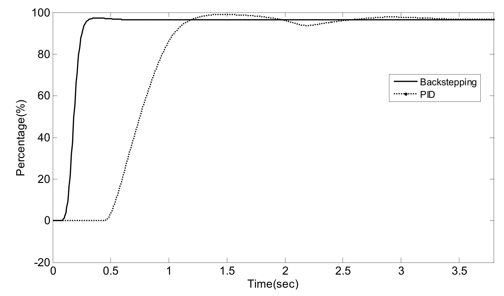
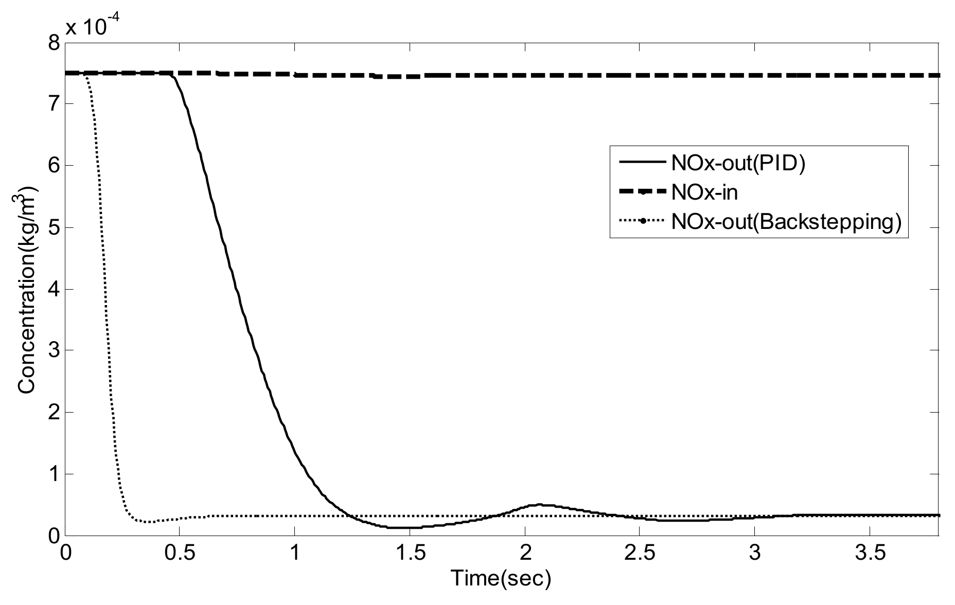
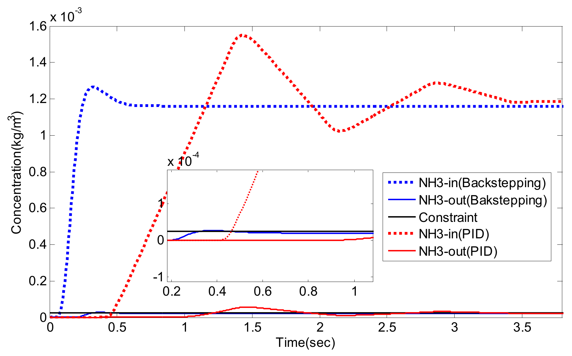
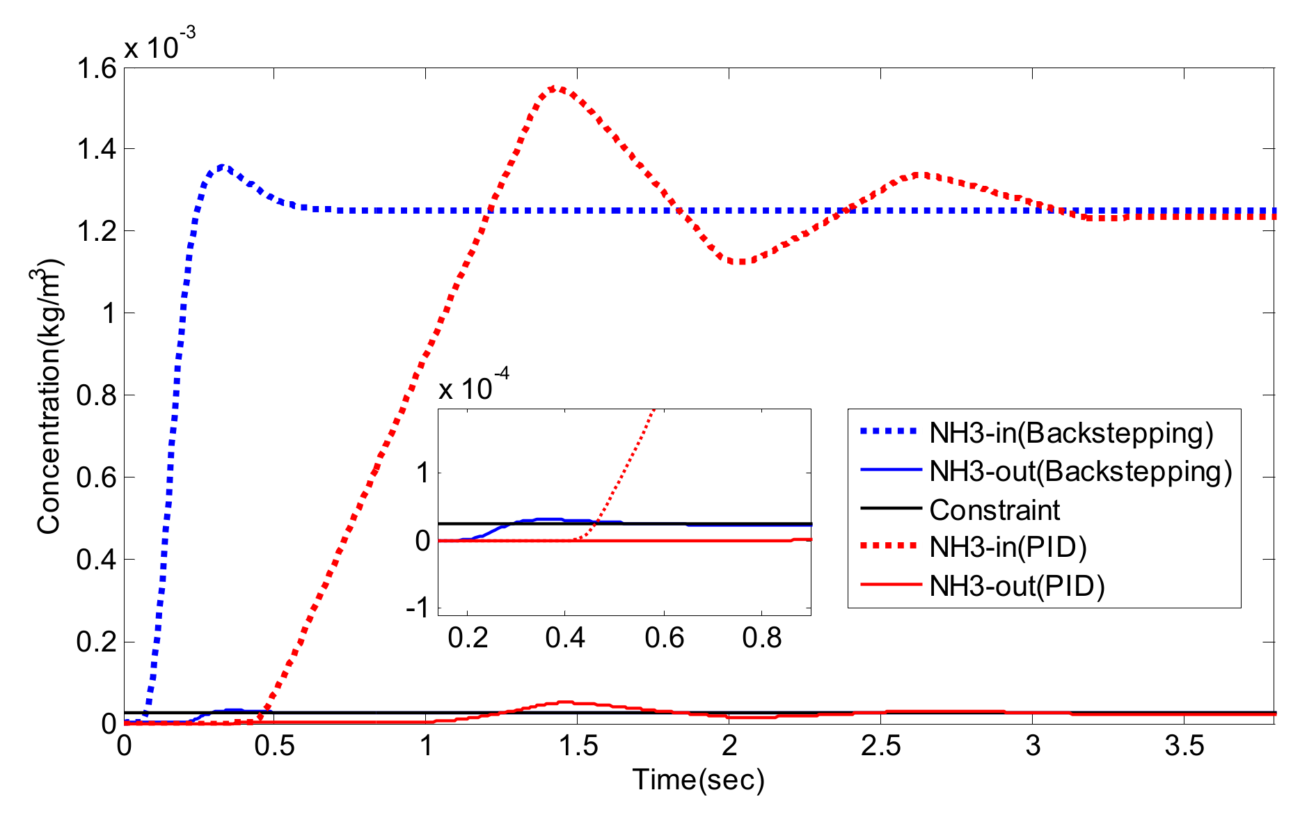
5. Experiment Results and Analysis

Several studies have reported that the combination of DOC (Diesel Oxidation Catalyst), DPF, and SCR has become one of the most common post-processing applications in heavy diesel engines, which can handle PM and NOx simultaneously [30,31,32]. Normally, DOC, installed upstream of the SCR catalysts, is utilized to convert part of NO into NO2. At the same time, DPF, installed between the DOC and the SCR, is used for reducing PM emissions. Figure 3 shows a schematic diagram of a SCR after-treatment system. The detail parameters of the parts are listed in Table 1, Table 2, Table 3 and Table 4.
According to the proposed algorithm, the schematic diagram of the control system is designed as shown in Figure 4. In the system, the NH3 concentration is estimated by the Luenberger-sliding mode observer and used as the input of the backstepping control. After that, the SCR is controlled by the controller.

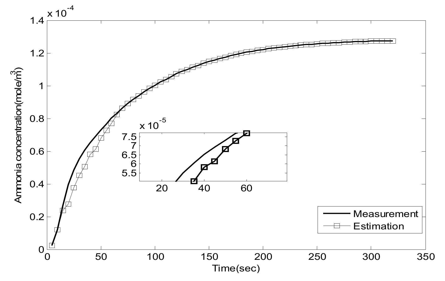
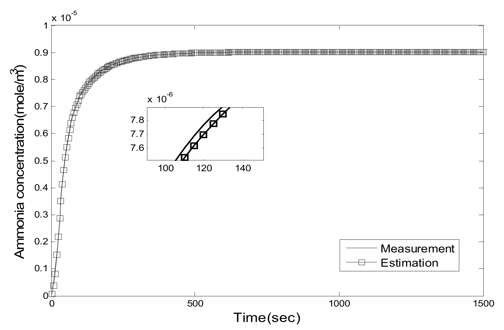
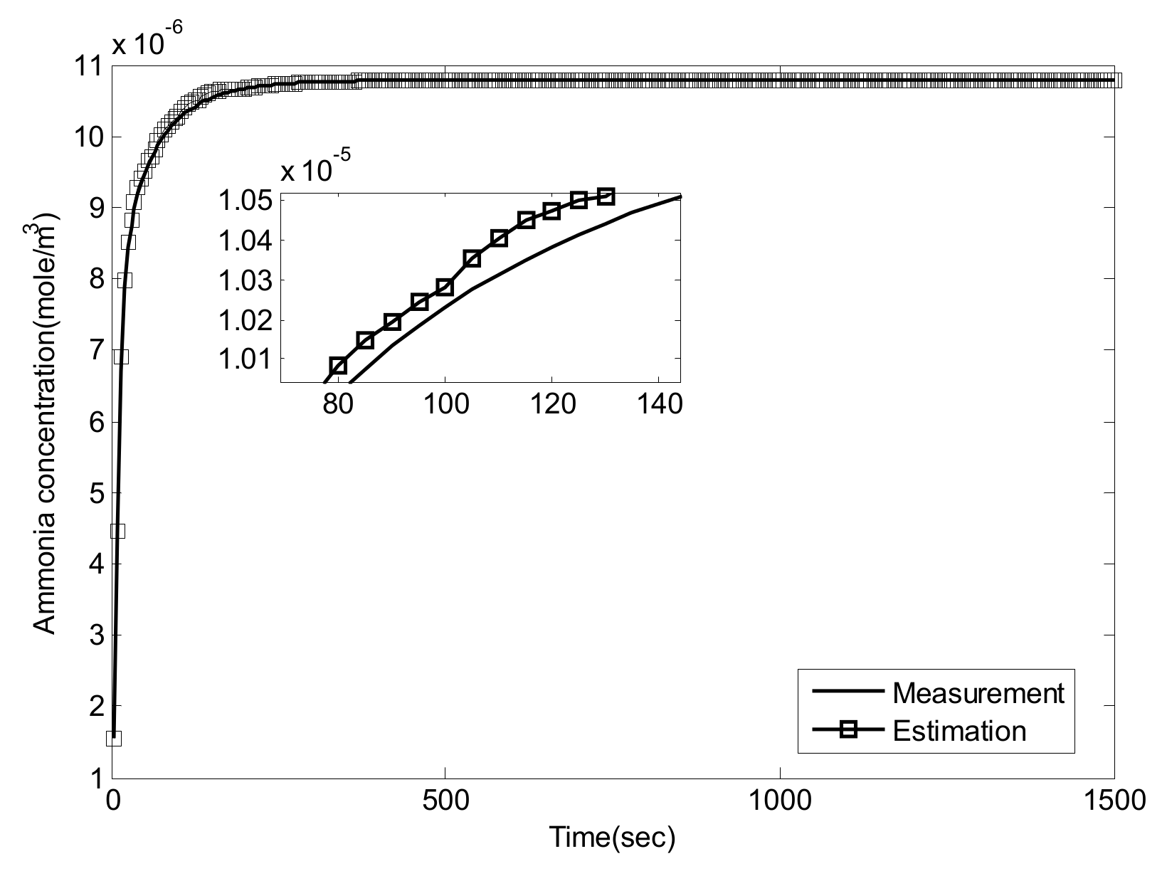
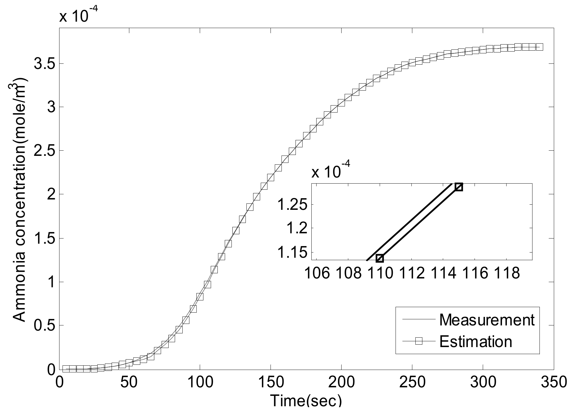
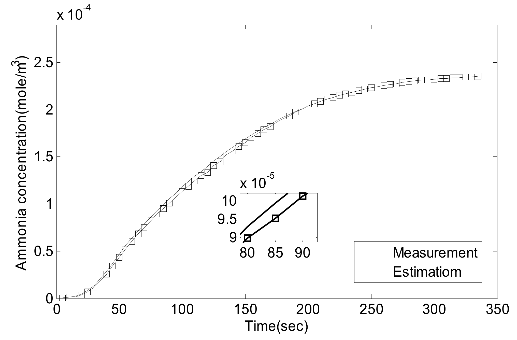
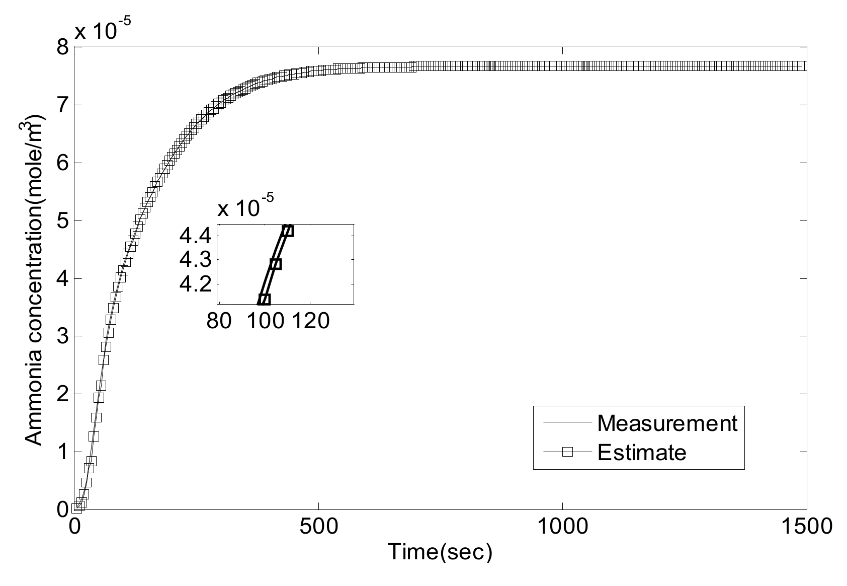
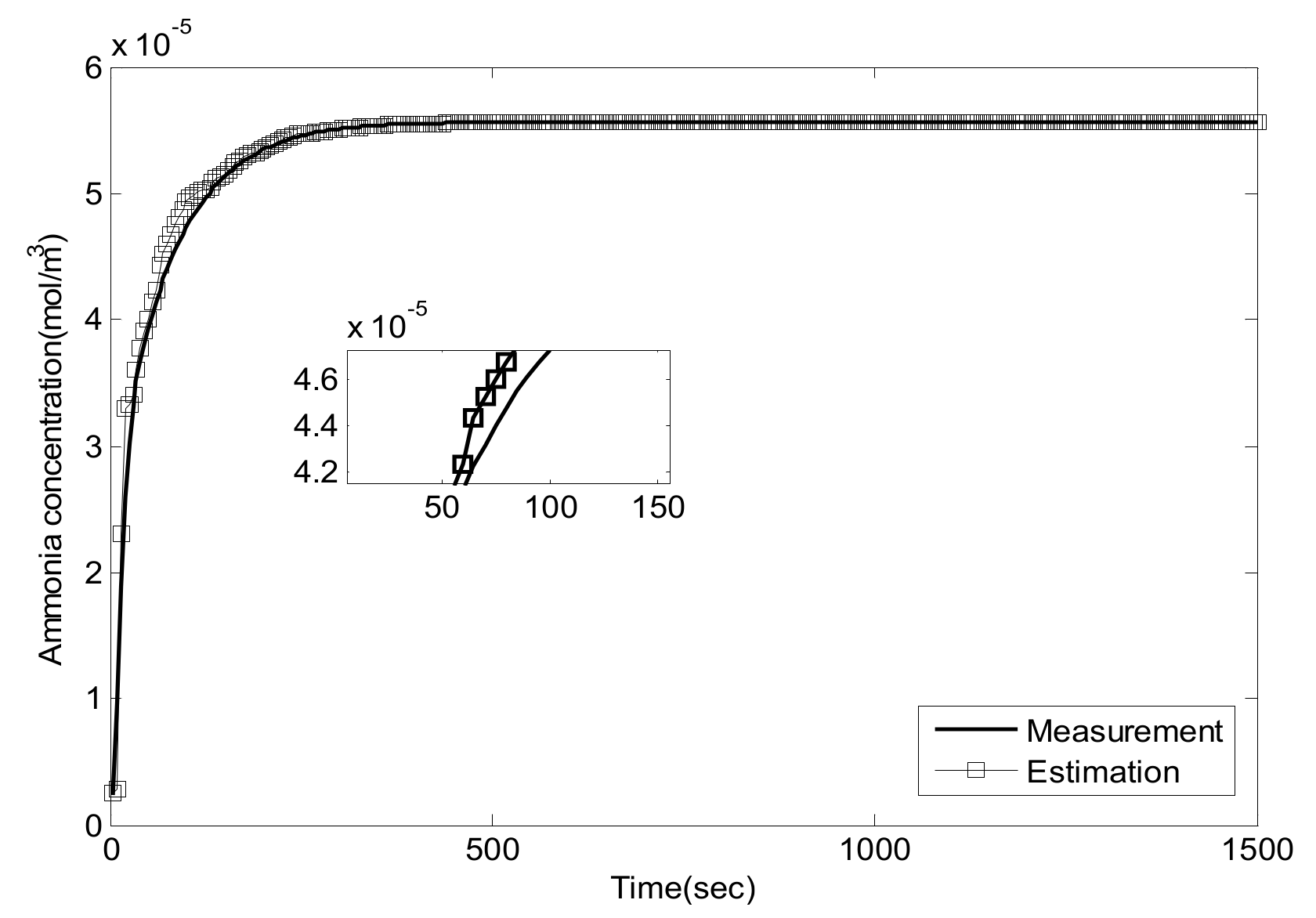
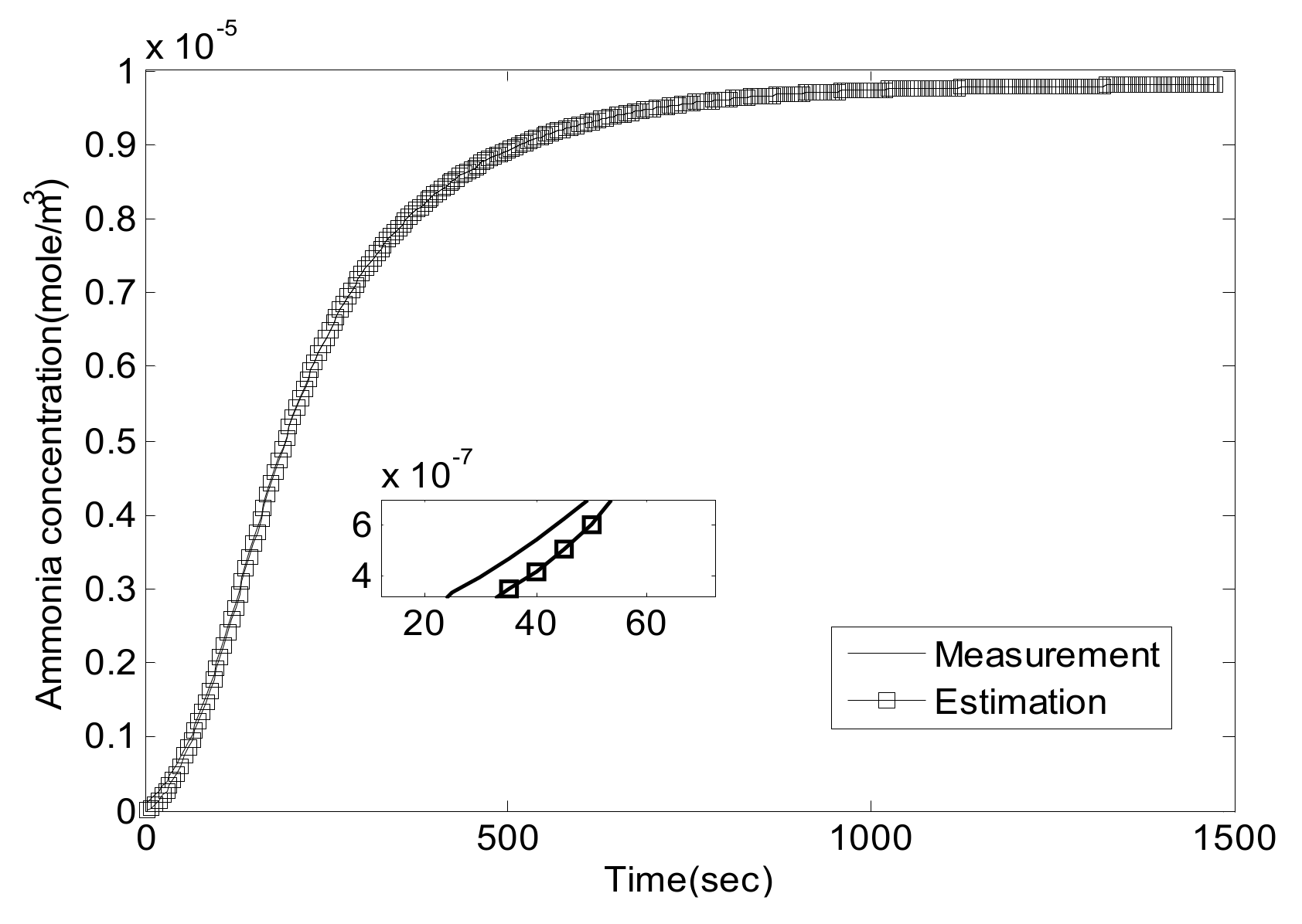
5.1. Experiment Validation of Luenberger-Sliding Mode Observer

In this section, the effectiveness of the observer will be validated first. Because the main reactions on the catalyst are standard reactions and fast reactions, as shown in (8) and (9), the simple model-based controller is targeting a molar ratio of NH3/NOX of 1/1 in order to suppress NH3 leakage. The observer result of the mid-catalyst NH3 concentration at three different NO2/NO ratios and different temperatures are shown in Figure 5, Figure 6, Figure 7, Figure 8, Figure 9, Figure 10, Figure 11, Figure 12 and Figure 13.
In order to show their performance more intuitively, the mean absolute error is given in Table 5.
As can be seen, the proposed Luenberger-sliding mode observer estimation can converge to sensor measurements very well at different working conditions. The experimental results show that the observation accuracy of mid-catalyst NH3 concentration can be achieved by using the proposed observer.

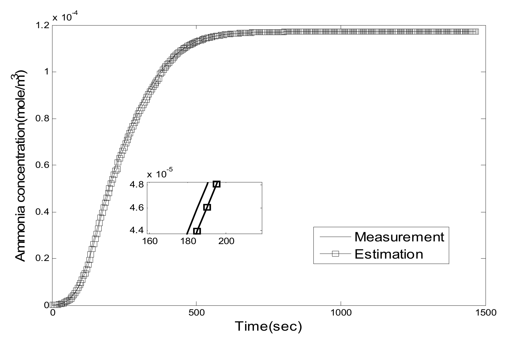
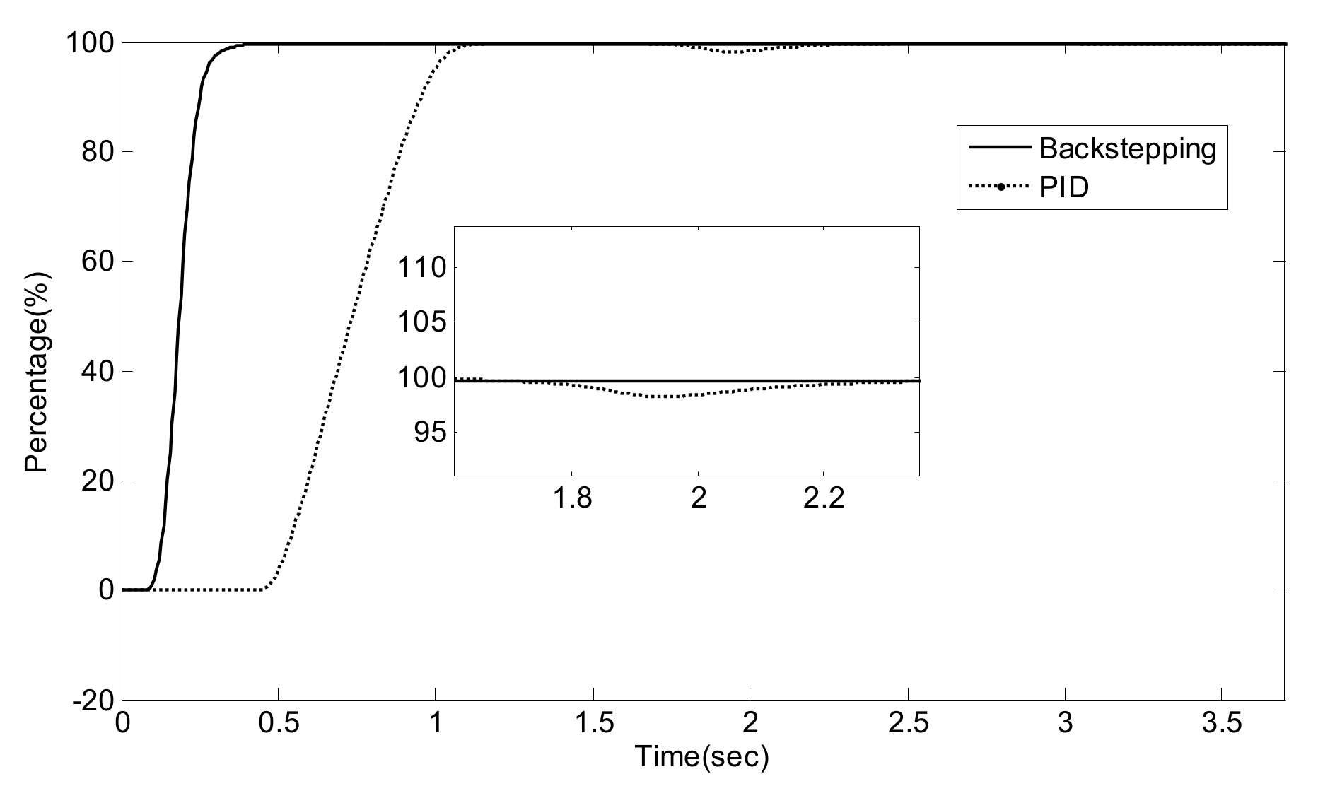
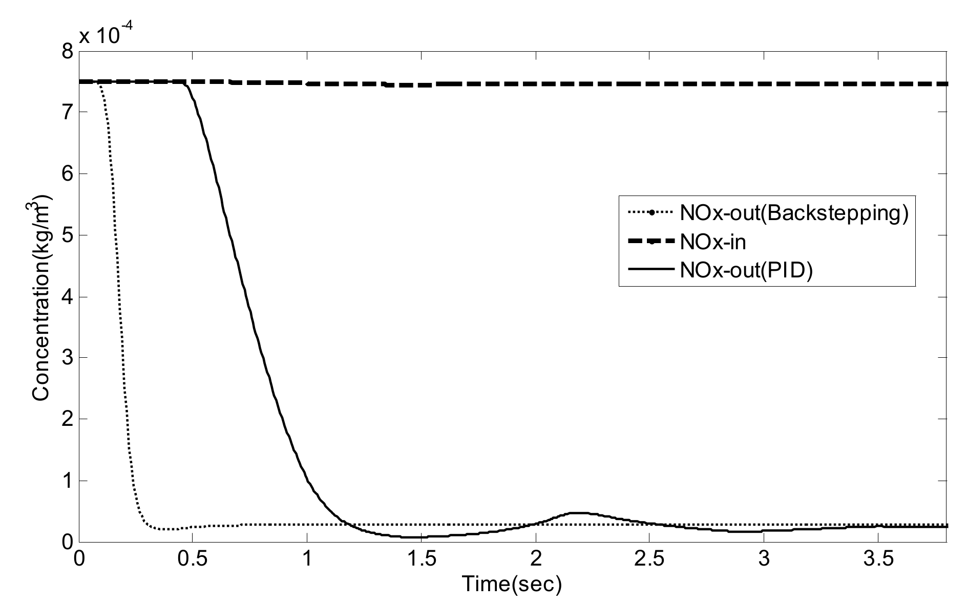
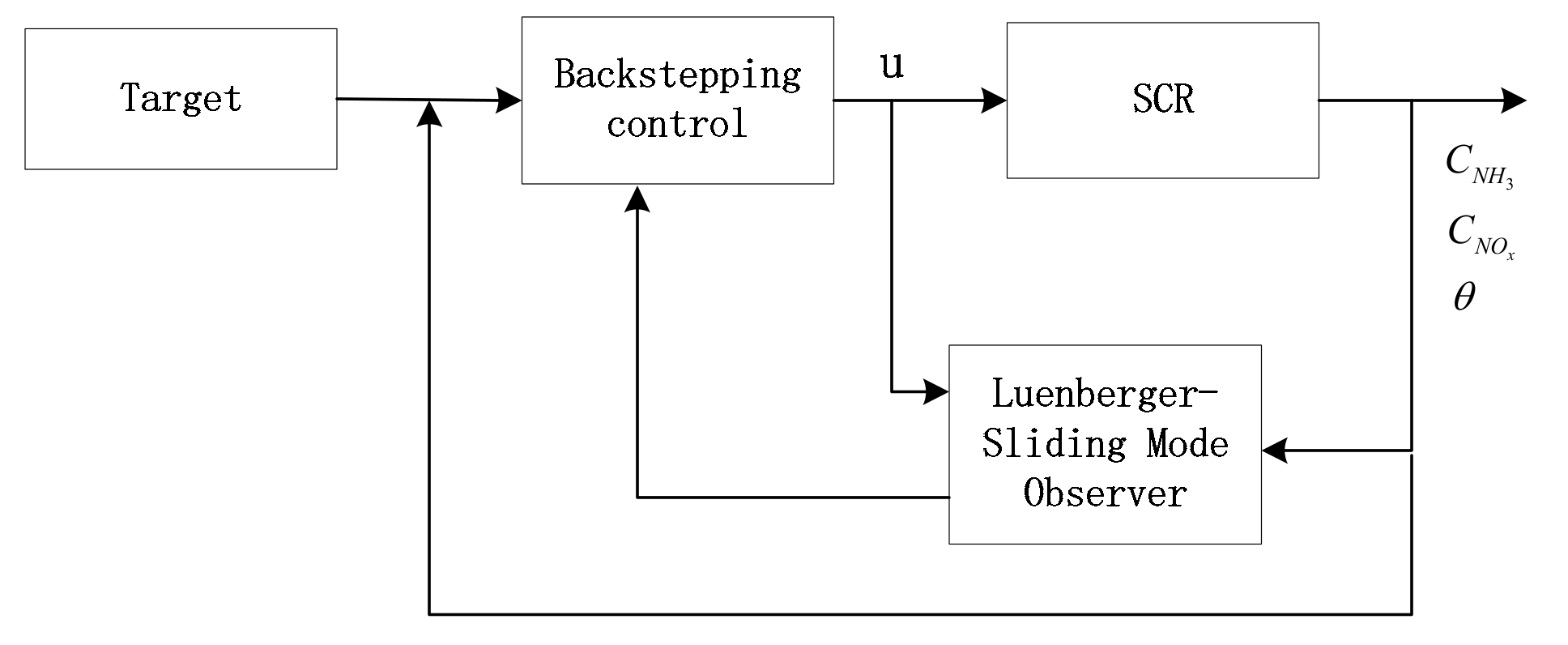
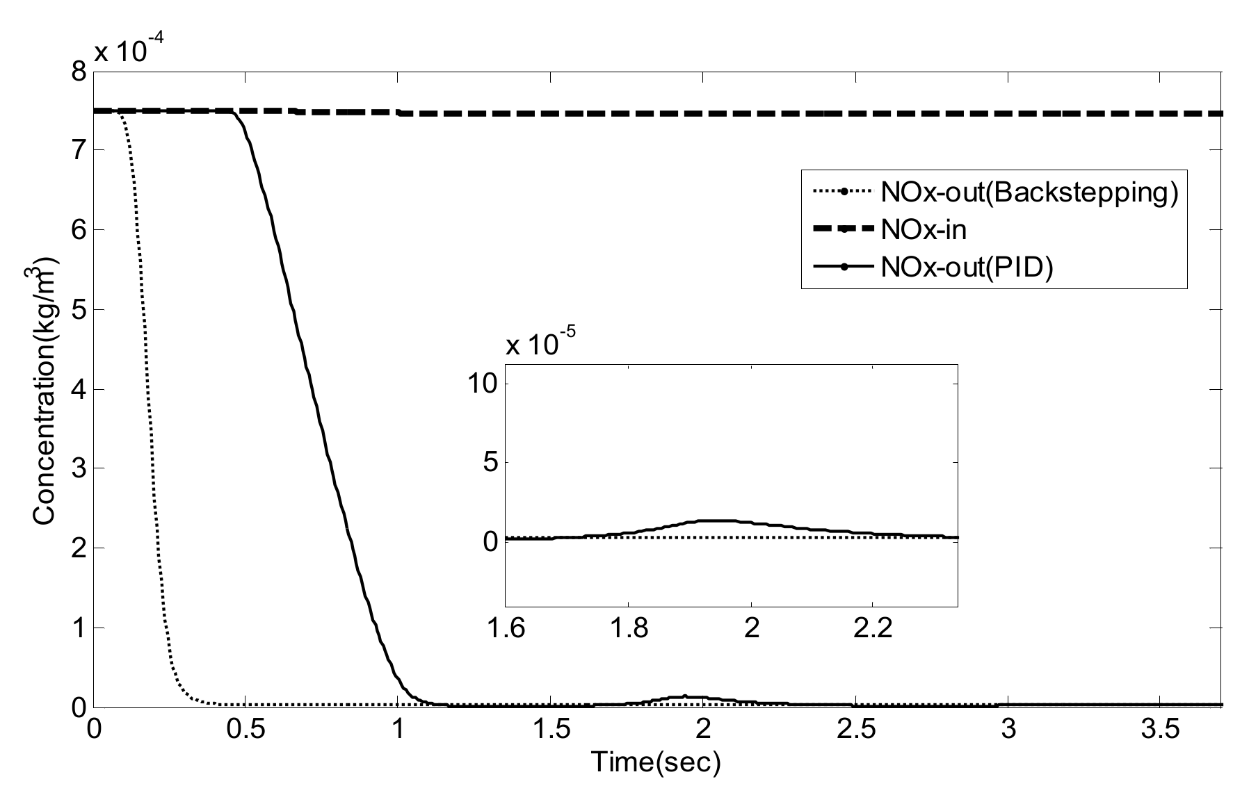
5.2. Simulation Validation of the Luenberger-Sliding Mode Observer Based Backstepping Control for SCR System

To illustrate the validity of the Luenberger-sliding mode observer based backstepping control for the after-treatment process, NOX conversion efficiency and NH3 leakage are taken as the output, and the injection of urea (concentration of the inlet ammonia) is taken as the input. To show the effectiveness of the proposed control strategy, traditional PID control is used for comparison. The control performance of the proposed Luenberger-sliding mode observer based backstepping control strategy is shown in Figure 14, Figure 15, Figure 16, Figure 17, Figure 18, Figure 19, Figure 20, Figure 21 and Figure 22. The control performance of the two control methods is compared using integrated absolute error (IAE) criteria:
I A E = e ( t ) d t
where e ( t ) is the error between the reference value and the actual process output. The value of IAE is enumerated in Table 6.
As can be seen from Figure 14, Figure 15, Figure 16, Figure 17, Figure 18, Figure 19, Figure 20, Figure 21 and Figure 22 and Table 6, traditional PID control and Luenberger-sliding mode observer based backstepping control can basically meet the control requirements, and both can achieve high NOx conversion rate when the NH3 leakage in the tail gas exceeds the standard, or when a small amount exceeds the standard. Nevertheless, traditional PID control has a large overshoot, which is when it injects excessive adblue into the engine exhaust in a short time. As can be seen from Figure 14, Figure 16 and Figure 19, NH3 emission from the SCR catalytic converter outlet fluctuates for a period of time, which does not meet the requirements of emission regulations. The proposed controller reaches better operating points in which about 96.2% of NOX is reduced while allowing about 24 ppm NH3 slip past the catalyst. Although the backstepping control method also has a small amount of overshoot, the downstream emission of the SCR catalysts does not exceed the limit, which is in line with the requirements of emission regulations. Moreover, the backstepping control method has a shorter adjustment time. Even in the case of overshoot, NH3 emissions downstream of the SCR catalyst can quickly return to normal levels, which is conducive to achieving a higher NOX conversion rate. Furthermore, the control response obtained using the Luenberger-sliding mode observer based backstepping controller has smaller overshoot and relatively shorter settling time. The control responses indicate the efficiency of the proposed controller with excellent set-point tracking properties.

6. Conclusions

In this paper, a Luenberger-sliding mode observer based backstepping control strategy was proposed to estimate the mid-catalyst ammonia concentration and calculate the input of adblue. The dynamics of a SCR system was modeled to represent the actual process in the design study of the Luenberger-sliding mode observer based backstepping control strategy. The Lyapunov technique was used for demonstrating the stability of the observer and the backstepping SCR control method. Through the simulation test, the performance of the Luenberger-sliding mode observer and the proposed approach was verified under the conditions of different intake components and different intake temperatures. The results show that the observer has high estimation accuracy under different conditions, with a maximum average error of less than 4.2 × 10⁻⁶. Furthermore, the Luenberger-sliding mode observer based backstepping control strategy can keep the ammonia slip of the downstream SCR system at a low level and simultaneously achieve a high NOX conversion rate, which is much better than the popular PID control method in setting time, overshoot, and tracking error.

Author Contributions

Conceptualization, T.Z.; Methodology, Y.L.; Software, B.Y.; Validation, Y.M.; formal analysis, Y.M.; Investigation, T.Z.; Resources, B.Y.; Data curation, B.Y.; Writing, T.Z.; Writing—review and editing, Y.M.

Funding

This research was funded by the Foundation and Frontier Projects in Chongqing, grant number cstc2018jcyjAX0684.

Conflicts of Interest

The authors declare no conflict of interest.

References

  1. Christoph, M.S.; Christopher, H.O.; Hans, P.G. Control of an SCR catalytic converter system for a mobile heavy-duty application. IEEE Trans. Control Syst. Technol. 2006, 14, 641–653. [Google Scholar]
  2. Yan, F.; Wang, J. Control of diesel engine dual-loop EGRair-path systems by a singular perturbation method. Control Eng. Pract. 2013, 21, 981–988. [Google Scholar] [CrossRef]
  3. Lee, S.; Park, S. Numerical analysis of internal flowcharacteristics of urea injectors for SCR dosing system. Fuel 2014, 129, 54–60. [Google Scholar] [CrossRef]
  4. Chen, P.; Wang, J. A novel cost-effective robust approach forselective catalytic reduction state estimations using dual nitrogenoxide sensors. J. Automob. Eng. 2015, 229, 83–96. [Google Scholar] [CrossRef]
  5. Devarakonda, M.; Parker, G.; Johnson, J.H.; Strots, V. Model-based control system design in a urea-SCR aftertreatmentsystem based on NH3 sensor feedback. Int. J. Automot. Technol. 2009, 10, 653–662. [Google Scholar] [CrossRef]
  6. Yan, F.; Wang, J. Design and robustness analysis of discreteobservers for diesel engine in-cylinder oxygen mass fractioncycle-by-cycle estimation. Control Syst. Technol. 2012, 20, 72–83. [Google Scholar]
  7. Ham, Y.; Park, S. Development of Map based Open Loop Control Algorithm for Urea-SCR System. Trans. Korean Soc. Automot. Eng. 2011, 19, 50–56. [Google Scholar]
  8. Zhang, S.M.; Tian, F.; Ren, G.F.; Yang, L.S. CR control strategy based on ANNs and Fuzzy PID in a heavy-duty diesel engine. Int. J. Automot. Technol. 2012, 13, 693–699. [Google Scholar] [CrossRef]
  9. Kim, Y.; Park, T.; Jung, C. Hybrid Nonlinear Model Predictive Control of LNT and Urealess SCR AftertreatmentSystem. IEEE Trans. Control Syst. Technol. 2019, 27, 2305–2313. [Google Scholar] [CrossRef]
  10. Zhao, J.H.; Hu, Y.F.; Gong, X.; Chen, H. Modelling and control of urea-SCR systems through the triple-step non-linear method in consideration of time-varying parameters and reference dynamics. Trans. Inst. Meas. Control 2018, 40, 287–302. [Google Scholar] [CrossRef]
  11. Yang, B.; Keqiang, L.; Ukawa, H.; Handa, M. Modelling and control of anon-linear dynamic system for heavy-duty trucks. Proc. Inst. Mech. Eng. Part D J. Automob. Eng. 2006, 220, 1423–1435. [Google Scholar] [CrossRef]
  12. Chang, Y.H.; Chan, W.S.; Chang, C.W. T-S fuzzy model-basedadaptive dynamic surface control for ball and beam system. IEEE Trans. Ind. Electron. 2013, 60, 2251–2263. [Google Scholar] [CrossRef]
  13. Chi, J.N.; DaCosta, H.F.M. Modeling and control of a urea-SCR aftertreatmentsystem. SAE Trans. 2005, 114, 449–465. [Google Scholar]
  14. Devarakonda, M.; Parker, G.; Johnson, J.H. Model-basedestimation and control system development in a urea-SCR aftertreatmentsystem. SAE Int. J. Fuels Lubr. 2009, 1, 646–661. [Google Scholar] [CrossRef]
  15. Liu, Q.F.; Chen, H.; Hu, Y.F.; Sun, P.Y.; Li, J. Modeling and control of the fuel injection system for rail pressure regulation in GDI engine. IEEE/ASME Trans. Mechatron. 2014, 19, 1501–1513. [Google Scholar]
  16. Westerlund, C.; Westerberg, B.; Ingemar, O.; Egnell, R. Model predictive control of a combined EGR/SCR HD diesel engine[C]. SAE2010 World Congr. Exhib. 2010, 13–15. [Google Scholar] [CrossRef]
  17. Ebrahimian, V.; Habchi, C.; Nicolle, A. Detailed modeling of the evaporation and thermal decomposition of urea-water solution in SCR systems. AIChE J. 2012, 58, 1998–2009. [Google Scholar] [CrossRef]
  18. Chen, P.; Wang, J. Observer-based estimation of air-fractionsfor a diesel engine coupled with aftertreatment systems. Control Syst. Technol. 2013, 21, 2239–2250. [Google Scholar] [CrossRef]
  19. Bonfils, A.; Creff, Y.; Lepreux, O.; Petit, N. Closed-loop controlof a SCR system using a NOx sensor cross-sensitive to NH3. J. Process Control 2014, 24, 368–378. [Google Scholar] [CrossRef]
  20. Davila, J.; Fridman, L.; Levant, A. Second-Order Sliding-Mode-observer for Mechanical Systems. IEEE Trans. Autom. Control 2005, 50, 1785–1789. [Google Scholar] [CrossRef]
  21. Foo, G.; Rahman, M.F. Sensorless sliding-mode MTPA control of an IPM synchronous motor drive using a sliding-mode observer and HF signal injection. IEEE Trans. Ind. Electron. 2010, 57, 1270–1278. [Google Scholar] [CrossRef]
  22. Kubinski, D.J.; Visser, J.H. Sensor and method for determining the ammonia loading of a zeolite SCR catalyst. Sens. Actuators B Chem. 2008, 130, 425–429. [Google Scholar] [CrossRef]
  23. Hsieh, M.; Wang, J. Sliding-mode observer for urea-selectivecatalytic reduction (SCR) mid-catalyst ammonia concentrationestimation. Int. J. Automot. Technol. 2011, 12, 321–329. [Google Scholar] [CrossRef]
  24. Hasan, S.N.; Husain, I. A Luenberger-sliding mode observer for online parameter estimation and adaptation in high-performance induction motor drives. IEEE Trans. Ind. Appl. 2009, 45, 772–781. [Google Scholar] [CrossRef]
  25. Sun, W.C.; Gao, H.J.; Kaynak, O. Adaptive backstepping control for active suspension systems with hard constraints. IEEE/ASME Trans. Mechatron. 2013, 18, 1072–1079. [Google Scholar] [CrossRef]
  26. Hamida, A.; Leon, J.; Glumineau, A. Experimental sensorless control for IPMSM by using integral backstepping strategy and adaptive high gain observer. Control Eng. Pract. 2017, 59, 64–76. [Google Scholar] [CrossRef]
  27. Hsieh, M.; Wang, J. A two-cell backstepping-based control strategy for diesel engine selective catalytic reduction systems. Control Syst. Technol. 2014, 24, 1504–1515. [Google Scholar] [CrossRef]
  28. Olsson, L.; Sjövall, H.; Blint, R.J. A kinetic model for ammonia selective catalytic reduction over Cu-ZSM-5. Appl. Catal. B Environ. 2008, 81, 203–217. [Google Scholar] [CrossRef]
  29. Zheng, T.; Han, W.; Li, Y.; Yang, B.; Shi, L. Luenberger-sliding modeobserver based ammonia concentration estimation for selectivecatalyst reduction system[C]. In Proceedings of the 2016 12th World Congress on Intelligent Control and Automation (WCICA), Guilin, China, 12–15 June 2016; pp. 3021–3026. [Google Scholar]
  30. Morandi, S.; Prinetto, F.; Ghiotti, G.; Castoldi, L.; Lietti, L.; Forzatti, P.; Daturi, M.; Blasin-Aubé, V. The influence of CO2 and H2O on the storage properties of Pt-Ba/Al2O3 LNT catalyst studied by FT-IR spectroscopy and transient microreactor experiments. Catal. Today 2014, 231, 116–124. [Google Scholar] [CrossRef]
  31. Shimizu, K.; Satsuma, A. Hydrogen assisted urea-SCR and NH3-SCR with silver–alumina as highly active and SO2-tolerant de-NOx catalysis. Appl. Catal. B Environ. 2007, 77, 202–205. [Google Scholar] [CrossRef]
  32. Doronkin, D.E.; Fogel, S.; Tamm, S.; Olsson, L.; Khan, T.S.; Bligaard, T.; Gabrielsson, P.; Dahl, S. Study of the “Fast SCR”-like mechanism of H2-assisted SCR of NOx with ammonia over Ag/Al2O3. Appl. Catal. B Environ. 2012, 113, 228–236. [Google Scholar] [CrossRef]
Figure 1. Schematic diagram of a selective catalytic reduction (SCR) system.
Energies 12 04270 g001
Figure 2. Two-cell SCR catalyst model.
Energies 12 04270 g002
Figure 3. Schematic diagram of SCR after-treatment system for simulation.
Energies 12 04270 g003
Figure 4. Schematic diagram of the control system.
Energies 12 04270 g004
Figure 5. NO2/NO = 0/1, 30 °C, comparison of C N H 3 , 2 .
Energies 12 04270 g005
Figure 6. NO2/NO = 0/1, 350 °C, comparison of C N H 3 , 2 .
Energies 12 04270 g006
Figure 7. NO2/NO = 0/1, 400 °C, comparison of C N H 3 , 2 .
Energies 12 04270 g007
Figure 8. NO2/NO = 1/2, 300 °C, comparison of C N H 3 , 2 .
Energies 12 04270 g008
Figure 9. NO2/NO = 1/2, 350 °C, comparison of C N H 3 , 2 .
Energies 12 04270 g009
Figure 10. NO2/NO = 1/2, 400 °C, comparison of C N H 3 , 2 .
Energies 12 04270 g010
Figure 11. NO2/NO = 1/1, 300 °C, comparison of C N H 3 , 2 .
Energies 12 04270 g011
Figure 12. NO2/NO = 1/1, 350 °C, comparison of C N H 3 , 2 .
Energies 12 04270 g012
Figure 13. NO2/NO = 1/1, 400 °C, comparison of C N H 3 , 2 .
Energies 12 04270 g013
Figure 14. NO/NO2 = 1/0, NOx concentration before and after the SCR system.
Energies 12 04270 g014
Figure 15. NO/NO2 = 1/0, NOx conversion efficiency.
Energies 12 04270 g015
Figure 16. NO/NO2 = 2/1, NOx concentration before and after the SCR system.
Energies 12 04270 g016
Figure 17. NO/NO2 = 2/1, NOx conversion efficiency.
Energies 12 04270 g017
Figure 18. NO/NO2 = 1/1, NOx concentration before and after the SCR system.
Energies 12 04270 g018
Figure 19. NO/NO2 = 1/1, NOx conversion efficiency.
Energies 12 04270 g019
Figure 20. NO/NO2 = 1/0, NH3 concentration before and after the SCR system.
Energies 12 04270 g020
Figure 21. NO/NO2 = 2/1, NH3 concentration before and after the SCR system.
Energies 12 04270 g021
Figure 22. NO/NO2 = 1/1, NH3 concentration before and after the SCR system.
Energies 12 04270 g022
Table 1. The detail parameters of the Engine.
ItemQuantity
Engine type4-cylinder
Bore (mm)100
Stroke (mm)110
Connecting rod length (mm)152
Compression ratio18
Engine displacement (liter)3
Table 2. Configuration parameters of SCR in GT power.
ItemQuantity
Cell density (1/inch2)400
Length (mm)250
Diamater (mm)25
Active surface site density (mole/m3)125
Table 3. Configuration parameters of DOC in GT-power.
ItemQuantity
Channel geometrysquare
Front area (mm2)20000
Cell density (1/inch2)400
Length (mm)150
Table 4. Configuration parameters of DPF in GT-power.
ItemQuantity
Trap diameter (mm)130
Filter wall thickness (inch)0.014
Channel length (mm)260
Inlet cell density (1/inch2)95
Table 5. Mean absolute error for Figure 5, Figure 6, Figure 7, Figure 8, Figure 9, Figure 10, Figure 11, Figure 12 and Figure 13.
NO2/NO = 0/1NO2/NO = 1/2NO2/NO = 1/1
300 °C1.9 × 10−61.6 × 10−61.1 × 10−7
350 °C3.1 × 10−61.7 × 10−60.6 × 10−7
400 °C4.2 × 10−62.1 × 10−61.6 × 10−7
Table 6. Control performance of the two control strategies.
NO/NO2Settling Time (s)Overshoot (%)Integrated Absolute Error (IAE)
PID1/03.227.80.1482
2/13.330.00.1784
1/13.125.20.1649
Luenberger-Sliding Mode Observer Based Backstepping1/00.499.30.0373
2/10.498.90.0295
1/10.488.30.0310

