Abstract
This paper presents a method to find the optimal configuration for an electric vehicle energy storage system using a cascaded H-bridge (CHB) inverter. CHB multilevel inverters enable a better utilization of the battery pack, because cells/modules with manufacturing tolerances in terms of capacity can be selectively discharged instead of being passively balanced by discharging them over resistors. The balancing algorithms have been investigated in many studies for the CHB topology. However, it has not yet been investigated to which extend a conventional pack can be modularized in a CHB configuration. Therefore, this paper explores different configurations by simulating different switch models, switch configurations, and number of levels for a CHB inverter along with a reference load model to find the optimal design of the system. The configuration is also considered from an economically point of view, as the most efficient solution might not be cost-effective to be installed in a common production vehicle. It is found that four modules per phase give the best compromise between efficiency and costs. Paralleling smaller switches should be preferred over the usage of fewer, larger switches. Moreover, selecting specific existing components results in higher savings compared to theoretical optimal components.
1. Introduction
Lithium-ion batteries are currently the most preferred energy storage solution for battery electric vehicles (BEV). For such vehicles, unfortunately they are also the biggest cost contributor with up to 50% of the manufacturing costs [1]. This results in the aim to use the battery as efficient as possible. In a conventional BEV battery pack, many cells, sometimes several thousand, are connected in series and parallel to increase the voltage, capacity, and current rating of the pack according to the requirements. Due to manufacturing tolerances, cells, even from the same batch, have different parameters such as capacity and internal resistance [2,3,4]. The capacity of in-series connected cells is limited by the cell with the lowest value because of the otherwise increased aging or safety problems caused by the over-discharge of that cell [5]. Parallel connections of cells with different parameters result in self balancing currents between the respective cells, which cause additional losses and aging [6]. Baumhoefer et al. [7] have shown that the cells with different initial capacities in a battery pack age differently over time, and the variation of capacities increases. An explanation for this is that putting the same load on weaker cells would degrade them faster as compared to the healthier cells [8]. These inconsistencies may limit the performance of a battery pack and reduce its lifetime.
Current solutions focus on additional circuits to balance the energy levels between the series connected modules, by either active or passive balancing [9]. However, independent of how effective such a balancing is, it results in additional losses, the batteries experience additional cycling and the circuits are causing additional costs. Utilization of the battery cell capacity cannot be increased by these methods. Extended effort during production and assembly of cells and packs can help to reduce the variations, but also increases the costs [10].
A modularization of the battery pack with individually controllable loads can enable a more individual dis-/charge for a higher utilization. There are various concepts being researched on how to modularize battery packs: direct, active interconnections [11], separate DC/DC converters for each module [12], or various multilevel converter designs [13]. For electric vehicles (EV), multilevel converters have been especially looked upon as an alternate topology compared to conventional two-level inverters, since they do not require additional hardware besides the inverter and offer a big benefit for the efficiency [14,15,16]. Advantages of modular multilevel converters (MMC) with embedded battery cells have already been demonstrated for electric vehicles [17]. The cascaded H-bridge (CHB) inverter, shown in Figure 1, is indicated as the preferred topology, when separate DC sources, like battery modules, are available to form submodules (SM) [14,18]. This is due to its low number of components, simple construction, and modular design.
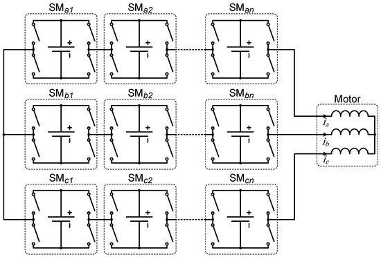
Figure 1.
Cascaded H-bridge circuit consisting of three phases with scalable number of sub modules.
The CHB circuit additionally seems to be one of the most promising solutions to target the cell parameter tolerances, since with this circuit, the individual modules can be implemented with low voltage metal–oxide–semiconductor field-effect transistor (MOSFET) switches, which are more efficient and cost effective than the conventional high voltage insulated-gate bipolar transistor (IGBT) switches [19]. Especially for the automotive use case, where the driving cycles provide a partial load scenario most of the time, this implementation can save energy. This can lead to the flexibility to decrease the battery capacity by still fulfilling the same range requirements. Additionally, this circuit enables improved output voltage waveforms, spread thermal loss sources, and a better operation in fault modes [20]. The overall change in the powertrain configuration can be seen in Figure 2.
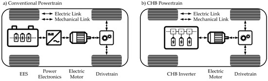
Figure 2.
Illustration of the overall electrical architecture of a (a) conventional powertrain and (b) cascaded H-bridge powertrain.
However, the work, which has been done in this field so far, does not include a comprehensive analysis of the costs and losses associated with different configurations of the CHB inverter, e.g., the number of levels, selection of switches, etc. There are setups described with only three levels [21] and up to eleven [14,22], twenty-one [23,24] or even twenty-three levels [25,26] with a big majority focusing on seven level CHB inverters [8,27,28,29,30,31,32]. Only one publication was found comparing different configurations, but only with regards to efficiency and without any cost consideration [33].
This paper aims to fill that research gap by providing a holistic model of an electric vehicle energy storage system using MATLAB/Simulink, which evaluates optimal parameters like module size, number of modules, switch parameters, and costs using a CHB inverter as compared to a static battery pack. For that, the model simulates driving cycles with different configurations and compares the efficiency and cost differences compared to a conventional power train.
2. Method
The approach to find the most suitable configuration is to simulate all possible configurations and identify the one with the lowest losses and costs. Therefore, first a longitudinal simulation model of an EV is defined, where all the involved components of a conventional electric powertrain are modeled. The different parameters are set to represent a current electric vehicle available on the market as a reference, which can be used for validation as well. Costs of the relevant parts are considered as well. Then, the same model is modified for a CHB powertrain with adjustable parameters and components. For the most relevant cost contributors, the switches, a cost model is defined to get realistic values depending on their parameters. By sweeping the values between the possible limits, an optimal configuration can be found. This comparison can be done either without cost consideration, with the best switch selected from a database or a theoretical optimal switch. Such a theoretical optimal switch is a non-existent component with electrical parameters that exactly fit the requirements, since commercial available switches only have these parameters defined with discrete levels.
The simulation model consists of three major components: the load, the inverter, and the costs. A block diagram of the simulation model can be seen in Figure 3. All these sub-models are modular and are explained in the following subsections. Where possible, existing sub-models from previous research and publications have been used.
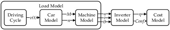
Figure 3.
Block diagram of the simulation model indicating the sub-models and forwarded variables.
2.1. Load Model
The load model can be divided into two sub-models: a car model and a machine model. The car model takes a selected driving cycle as an input. There are various driving cycles currently in use to have a defined, yet realistic, load input. Different driving cycles map different scenarios, from urban driving to expressway including combinations of them. The built model accepts any, as it just requires a speed over time data. The following calculations are all based on the worldwide harmonized light vehicles test procedure (WLTP) class 3 cycle, since it is used as a reference by many countries and includes low, medium, high, and extra high velocities [34].
With this input, the car model determines the torque and rotational speed requirements for the electric machine. Factors like the vehicle mass, transmission ratio, and transmission losses are considered and can be taken from vehicle datasheets. For this paper, the selected reference vehicle is the BMW i3 B-segment hatchback car with the 94 Ah battery, as it is a good example of an urban vehicle with many parameters publicly available [35]. It is still considered one of the most efficient EVs despite being on the market for many years [36]. Any other vehicle can be implemented instead, if the necessary parameters are available. The vehicle model, which is adapted for this work, is originally described in detail and validated in [18].
The machine model takes this as an input to determine the required voltage, current, and power factor from the inverter to operate at the defined conditions. The installed motor from the reference vehicle is used to parametrize the machine model, which is a permanent magnet synchronous machine (PMSM) with a rated power of 125 kW. Also, this model is adapted from the already validated model in [18].
2.2. Inverter Loss Model
The outputs from the load model are directly used to calculate the losses in the inverter, which converts the direct current (DC) of the battery into alternating current (AC) to drive the motor. The switches used in the inverter are causing conduction losses and switching losses. The CHB inverter proposed in this research uses individual switches, which are implemented by silicon-based MOSFET switches. To calculate the losses per switch, a validated simulation model is used [18,37], which is based on 12 parameters that can be extracted from the MOSFET datasheets. These are drain-source voltage , drain current , temperature coefficient , drain-source on resistance , dynamic resistance of the anti-paralleled diode , diode on-state zero-current voltage , recovered charge of the anti-paralleled diode , gate-drain capacitance , gate-drain capacitance , plateau voltage , current rise-time during turn-on , and current fall-time during turn-off . Especially for the cost comparison, a reference to a current state of the art inverter is required. So a second model is used, which simulates the efficiency of the original IGBT inverter used in the reference vehicle.
The switch parameters used for the simulation are collected in a database with a total of 63 different MOSFETs. The switches are selected to create a relevant overview of automotive and consumer electronic switches with a wide range of blocking voltages, conduction/switching losses, costs, and manufacturers. For parameters regarding the maximum blocking voltage, a de-rating factor of 0.8, and for the maximum current a de-rating factor of 0.75, are used according to IPC9592 [38].
The CHB inverter model then uses the simulation of the individual switches. For this, only the 3-phase configuration is considered to ensure a compatibility with current state-of-the-art motors. Each phase can have varying number of modules. The smallest number of modules is one resulting in a three-level inverter and the rated cell voltage and rated motor voltage define the largest possible number. For the reference vehicle, the battery is rated at 360 V, which can be implemented with up to 50 modules resulting in 101 levels in phase voltage. Each module needs four switches for the H-bridge configuration, but each switch can consist of several parallel connected MOSFET to ensure the required current capability of up to 400 A.
To find the theoretical optimal switch, a relation between the individual MOSFET parameters was investigated. The search for a theoretical optimal switch is required because the parameters of commercial components are only available in discrete levels. So there is a possibility that an optimal value is just slightly above a discrete value, but because of this, the next higher level has to be selected, which could influence the costs or efficiency disproportional. To implement the model to find this theoretical optimal switch, first a sensitivity analysis of the loss concerning the switch parameters was analyzed. The voltage and current were excluded from the analysis as the number of series- and parallel-connected switches directly defines these values. All the remaining ten parameters were individually multiplied with a factor starting from 0 and then increasing by 0.2 until reaching the value 2. The used configuration for this analysis was defined with three modules and two parallel switches with the MOSFET IPT020N10N3 from Infineon, which is an optimum configuration within its cost category. The result of this analysis, as visible in Figure 4, is that only (46.3% slope), (15.9% slope), and (19.2% slope) have a significant influence with a slope of more than 10% on the efficiency. Other parameters do not influence the losses significantly, if they are changed. Therefore, only these three parameters have to be adapted (besides and , which are defined by the configuration) to find an optimal theoretical switch.
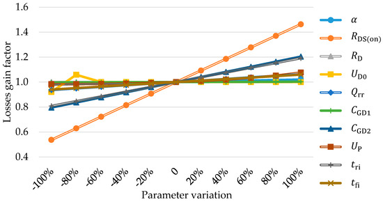
Figure 4.
Sensitivity analysis of losses against switch parameters.
The functions to find dependencies for the three parameters of the theoretical optimal switch are derived from the compiled switch database, where all the existing parameters are compared to each other. It has to be mentioned that these dependencies are not correlating with large fitting factors, which indicates rather weak relations. Nevertheless, they indicate the general behaviour therefore are used here.
The drain-source on resistance influences the efficiency the most, where a doubling of the value will increase the losses by almost 1.5. This is because the conduction losses of the switch are defined by it. The resistance depends on many different conditions, which cannot be projected in a simple model for this research. However, amongst the 63 switches included in this research, a linear relation with the drain-source voltage was found with a coefficient of determination of 50.39%, as can be seen in Figure 5.
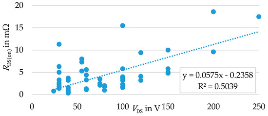
Figure 5.
Relation between the voltage and the resistance of the selected switches.
The switching loss is equally caused by the current rise-time and gate-drain capacitance and majorly depends on the switching frequency, which is defined to be 20 kHz for the CHB inverter. Like for the resistance, these are factors determined by many different conditions in the way the MOSFET is designed. Yet with the limited dataset, linear approximations are possible, when the values are plotted in relation to the current . It results in coefficients of determination of 46% for the capacitance as seen in Figure 6. For the current rise-time, the coefficient of determination is not very strong with 29.21% as seen in Figure 7, but since the sensitivity is also rather weak and just above the threshold, it is still considered usable.
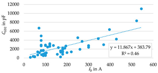
Figure 6.
Relation between the current and the capacitance .
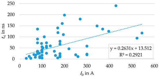
Figure 7.
Relation between the current and the rise-time .
Based on the analysis of these configurations with different switches, numbers of levels and the number of parallel switches, the most suitable configuration for a CHB inverter, can be selected depending on evaluation criteria like efficiency, cost savings, or a combination of them.
2.3. Cost Model
The cost is an important factor to consider for an optimal system, which is feasible to be implemented in an automotive environment. Without a cost consideration, many optimized parameters would indicate unrealistic trends. For example, the number of parallel switches would be infinite, as the conduction losses decrease linear with their amount. On the other hand, the evaluation of the cost is not straight forward, since it is not possible to get access to the real numbers an original equipment manufacturer (OEM) would pay for its components. Prices from various distributors, which are available online, include additional influencing factors like demands, promoting sales, etc., which do not allow a direct comparison between multiple components.
The approach of this publication regarding the cost is not to identify the exact cost of the whole powertrain, but to investigate the change in the costs of the components for the power train with an IGBT inverter and a CHB inverter. The most sensitive parts for that are actually the switches [39,40], which is why major attention is put on their costs. To indicate various possibilities, five different approaches are adopted to model the costs of switches.
The first approach is the usage of a comparing web page, which includes several major distributors of electronic components [41]. There, the value of a quantity of 1000 pieces is used, since not all components have a further price reduction with 10,000 pieces. These prices tend to be on the higher side since the distributors target end customers with lower quantities and therefore this first category is labelled as “HC Model” (high cost model).
The second category is defined accordingly with the label “LC Model” (low cost model), as here for each component, the lowest possible price is collected. No restriction was set for quantity or source. Often these low prices can be found on various e-commerce platforms, where the originality or new-status cannot directly be confirmed. Because of this, these values have to be considered with care, but indicate the possible magnitude for low prices. All prices are converted to USD as a common base currency, using the exchange rates stated in [1], and are rounded to integers.
Both these categories “HC Model” and “LC Model” strongly indicate the previously mentioned cost fluctuations independent from the product parameters. Therefore, the third category follows the systematic approach from Burkart et al. [39], who were able to link the costs of power electronic semiconductors to the surface area of the die and the packaging:
where is the specific price per chip area depending on the chip technology and is the package price including chip integration and bonding. As Burkart et al. do not indicate a specific price factor for Si MOSFET, the 600 V Si PIN diode value is used, since its semiconductor structure and manufacturing process are the closest. The package price stated in [39] is only given for rather large modules, but it indicates a power trend line depending on the package surface area with a coefficient of determination of 99.56%. The equation of the power trend line was used to extrapolate the costs of smaller packages for this research with the surface area from the datasheets to define . Results generated with Equation (1) are categorized under the third label “DSC Model” (die size cost model), which normally gives a cost somewhere between the “HC Model” and the “LC Model” category. For around 20 MOSFET switches, the required surface area of the semiconductor could be identified over their corresponding bare die datasheets. For a few relevant switches (seven in total), where no die size was available in the datasheets, samples were ordered and then opened to be able to measure the die size as seen in Figure 8. In the center bottom of Figure 8 it can be seen that some switches use the same packaging TO-220, but have a very different die size and therefore dissimilar parameters.
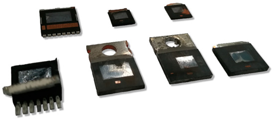
Figure 8.
Opened switches from different manufacturers and with different electric parameters.
It was not possible to find bare die datasheets or order samples for all switches from the database due to financial, time, and availability constraints. So, a fourth category was established with own cost modelling. For that, a linear relation was found between the product of the drain-to-source voltage multiplied with the drain current and the die surface area for the 20 switches, where the bare die datasheets were available. The coefficient of determination for the relation is 88.55% and the average absolute error is 7.46% as seen in Figure 9. With this, using the values of and , which are always available in the datasheets, a surface area can be calculated and therefore a cost estimation according to [39] is possible the same way as the “DSC Model” category. The packaging costs again can be calculated with the package surface area, which is always in the datasheets, and the extrapolation of packaging costs from Burkart et al. [39]. This category is called “VIC Model” (voltage-current cost model).
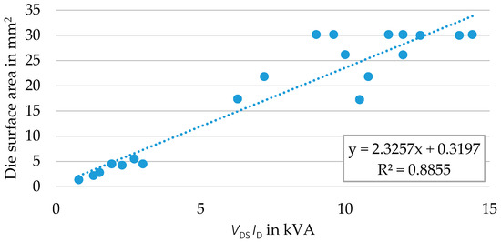
Figure 9.
Relation between the product of the drain-to-source voltage multiplied with the drain current and the die surface area.
The final category considers the costs for the theoretical optimal switch with no fixed restrictions and is therefore labelled as “Theoretical Optimal Switch Model” (TOS Model) category. It follows the cost calculation of Equation (1) and the cost definition of the “VIC Model” category for the die cost. The voltage and current are defined by the amount of series and parallel connected switches, which directly leads to the die surface area according to Figure 9 and therefore to a die cost according to Burkart et al. [39]. The packaging cost for such a theoretical switch is not directly derivable, as any trend line approximation approach failed for the investigated switches. As it also can be seen in Figure 8, the package area is not directly related to the die surface area and therefore the electrical parameters. This is the case since equal and similar package sizes can have very different die sizes and therefore parameters. The package selection during the design of mass manufactured switches is influenced by other factors like intended soldering/mounting technology, cooling strategy, and manufacturing handling. Therefore, it can be seen that among the selected switches most come in a packaging size of around 1 cm2 independent of any other parameters. To still be able to find a theoretical optimal MOSFET, it was defined that the package surface area must be bigger than the die surface area by a certain ratio to safely cover the sensitive semiconductor. It was investigated that among the switches with available die surface area, ratios of 3% to 44% with an average of 20% can be found. To find theoretical optimal switch for this research, the highest value of 44% was taken for them, as it indicates that it is possible to manufacture this ratio safely within the packaging technologies of the selected switches. Since the switch BSZ16DN25NS3 from Infineon with this ratio has a voltage rating = 250 V, which is the highest amongst the selected switches, it also can be ruled out that such a ratio is prohibited by voltage break-through requirements. Higher ratios of 80% with DirectFET packaging [42] and even up to 100% with chip scale packaging (CSP) [43] are possible, but this would make the results not directly comparable to the other cost models of this research.
To summarize the cost impacts of the different cost models, Table 1 gives an overview of the minimum, maximum, and average costs within the selected switches. The TOS model is excluded here, since its cost depends on the required specifications, and these specifications depend on the configuration of the CHB inverter.

Table 1.
Summary of the switch cost models.
Besides the switches, there are some other components which would be different in an automotive CHB inverter compared to an equivalent IGBT inverter, and therefore have to be considered from a cost perspective. Since the CHB modules are connected in series and there is no reference ground possible, each switch needs an isolated power supply, implemented with an isolated DC/DC converter. Additionally, the MOSFET requires drivers that can source and sink the currents to enable fast switching. Per switch, a cost of USD 4.5 is considered for the converter, USD 2 for the driver, and USD 0.45 for additionally required cooling efforts [18]. On top of that, an extensive controlling and communication network is necessary to align all the modules. An overhead of USD 300 is assumed to cover in a worst case scenario [18]. To account for the cost of manufacturing and assembly, the component costs have to be multiplied with an overhead cost factor, which can be found as 1.25 for power electronics converter production [40].
Because an analysis of the cost difference compared to a conventional IGBT inverter of the reference vehicle is the goal of this research, the costs for the IGBT components, which are not necessary anymore, have to be deducted. This cost derivation of them is discussed in detail in [18] and concluded as USD 666.5 for all the obsolete components. Another cost difference consideration are the contactors for the battery pack in the reference vehicle. Due to the nominal voltage of 400 V, which is higher than the defined DC safety threshold of 60 V, there have to be two contactors in the battery, one for each pole [44]. These components are assumed with USD 74 in the IGBT-driven vehicle [18]. For the CHB inverter, this is not necessary, as each module output is already without potential once the H-bridge is deactivated. On top of that, the voltage of each module is much lower compared to the conventional battery pack. Therefore, no extra cost is applied for the CHB inverter vehicle for contactors. The cost difference between an IGBT inverter driven vehicle and one with the usage of a CHB inverter can be expressed with:
where is the sum of all relevant costs of the IGBT inverter, is the costs for both contactors, and is the sum of all relevant costs for a CHB inverter including the switches.
Besides the cost difference for the components, there is an additional difference for the costs regarding the battery, as the CHB inverter can be more efficient depending on the configuration. This will enable the same range with a smaller battery capacity. It can also result in a bigger range with the same capacity, but this additional range is not directly comparable with the conventional system, as the range cannot be expressed directly in a higher value and therefore, price of the vehicle. To calculate the cost difference of the smaller battery, the difference in energy consumption is multiplied with the range requirement (the same range declaration as for the initial reference vehicle) and the cost of battery cells per capacity:
where is the average energy loss for the respective inverters, the range requirement, and is the cost per kWh for the battery on pack level. The loss of the IGBT inverter from the reference vehicle is simulated with the simulation mentioned in Section 2.2 as 1.22 kWh/100 km for the WLTP driving cycle, while the loss for the CHB inverter depends on the configuration. The range for the selected reference vehicle is officially declared with 300 km [45]. Current cost prediction of lithium-based battery packs with 18,650 cells or similar are considered with USD 164.28 per kWh [1].
Increased energy efficiency additionally has the benefit of reduced energy consumption during the lifetime, which also can be converted directly into saved costs if the total cost of ownership (TCO) is considered. Such a cost savings can enable a CHB configuration with higher costs, if the higher efficiency would compensate it and therefore is included in this research. These running costs are calculated with the average energy consumption multiplied with the costs for electricity and the estimated lifetime driven distance:
where is the average energy consumption for the respective inverters, the total driven distance over the lifetime, and the cost for the electric energy. The consumed energy for the IGBT inverter again is calculated with the Section 2.2 mentioned model and is 13.26 kWh/100 km for the reference vehicle and variable for the CHB inverter depending on the configuration. The total driven distance can be defined until the vehicle is damaged/aged beyond repair. For electric vehicles, the battery due to its aging behavior might be the limiting factor, as a replacement might not be economical [1]. However, the end-of-life duration is hard to estimate as it depends on many external factors like climate, charging/driving behavior, etc. A warranty of 100,000 miles (160,934.4 km) is given for the battery of the reference vehicle [46], which can be considered as a minimum life distance the vehicle is able to be driven until the defined end of life. However, a realistic number is probably much higher in most cases. In the datasheet of the Samsung SDI 94 Ah cell, which is the used cell type for the reference vehicle [47], a cycle life of at least 3200, but up to 4600 cycles is stated [48]. The minimum specifications of 3200 full cycles from the datasheet are used for the calculations of for this research. It results in a total driven distance of 960,000 km until end of life of the battery, which is considered feasible by current research [49]. The costs for electricity are varying greatly in different countries depending on many external factors. This research considers the costs from Germany in 2015 with USD 0.26 per kWh [1]. Germany is selected as a developed country without excessive access to own energy resources, but yet a high share of regenerative energy. Compared to other countries, this is a rather high price, which therefore is believed to not strongly be influenced by subsidies. The overall possible savings are the sum of the mentioned cost savings:
This formula is used to find the best possible configuration for the CHB inverter, where initial costs are balanced out the best with the higher efficiency and therefore savings. All possible configurations and combinations are simulated with a selected driving cycle and the benefits are calculated. The results are then sorted to see the best 100 possible configurations with their individual gains.
3. Results
The here presented results are all simulated with the WLTP C3 driving cycle. The limits are set to simulate all possible combinations of the 63 switches, from one to 50 modules per phase and from one to 30 parallel MOSFET for each switch. This results in 94,500 possible configurations, where each one is simulated with a whole driving cycle to model the energy consumption.
3.1. Maximum Theoretical Savings Consideration
In this first category, there are no hardware costs considered. Therefore, the simulation searches for the configuration with the highest overall energy efficiency. This, of course, will lead to economically unfeasible parameters, where even physical problems can occur for the implementation. Nevertheless, the results give some interesting insights in the overall trend of the optimum configuration and additionally define a threshold for an overall maximum theoretical achievable efficiency.
Switch: Without cost consideration, the simulation prefers switches with both small conduction resistance and charge capacitances, which reduce the conduction and switching losses. Throughout the first hundred best configurations, the switch BUK9J0R9-40H made by Nexperia is the preferred choice for 89 configurations.
Modules: From the possibility range without cost consideration, medium numbers of 17 to 18 are indicating the highest efficiency with 17 at the top. For the best 100 configurations, the lowest number of modules is 10, the highest 27, and on average 17.45. The highest occurrence in the top 100 is 13 modules per phase (12 times).
Parallel: As it could be expected, the highest number of parallel connected switches is the most efficient. To keep the calculation time low, a maximum of 30 parallel switches was set, which is therefore also the most efficient configuration. In the best 100 configurations, the lowest would be 19, and on average 26.56 parallel switches with 30 as the most occurring value (17 times).
Efficiency: The optimum configuration reaches very high levels of efficiency, which can be seen as a benchmark. The highest value is 99.80% and on average for the best 100, it is still 99.77% compared to the 93.65% for the IGBT inverter. Such an increased efficiency could make the battery pack up to 3.55 kWh and on average 3.54 kWh smaller.
Cost: Due to the high numbers of levels and parallel switches, such an optimal inverter would theoretically cost between USD 3726 and USD 13,031, more than the comparable IGBT inverter with an average additional cost of USD 7422 for the 100 best configurations. Any efficiency savings cannot compensate such a high cost, even during the whole lifetime. The savings on both battery size reduction and running costs would be rather independent from the configuration for the best 100 selections, on average USD 3476 and up to USD 3488, which also indicates the top benchmark for further results. The numbers shown in Figure 10 indicate only the theoretical savings without any hardware costs. On top of that, it has to be mentioned, that such a configuration might not be suitable for implementation due to packaging space and other constraints.
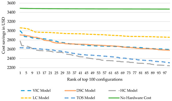
Figure 10.
Cost savings of the best 100 configurations for the four different categories.
3.2. Optimal Results with “HC Model” Cost Consideration
Using the “HC Model” cost category for the switches and the other costs as previously explained, very different configurations are found as an optimum. As this category is based on costs found online, it has to be considered with care, as there could be switches, which are sold with a lower/higher price compared to their parameters due to external factors.
Switch: The best switch for this configuration is the IAUT260N10S5N019 made by Infineon. Within the top 100, the most used switch (27 times) is IPP180N10N3, which is made by Infineon as well. Both switches have a rather high maximum voltage rating of 100 V, which allows a CHB inverter with only a few modules and therefore hardware costs lower than the IGBT inverter. So even though the costs are high, this configuration is still more cost efficient than the IGBT inverter.
Modules: The number of modules is now much lower compared to the previous category, as the switches are more costly. The first top nine configurations all work in a three module configuration. For the top 100, values from three to six are found with three the most common (43 times) and on average, 4.08 modules per phase.
Parallel: How many switches are connected in parallel now varies a lot, depending on the switch parameters. In the top 100 configurations, from two to the maximum 30 parallel switches, are found with an average of 11.67 and the most common configuration of seven (9 times).
Efficiency: The average and maximum efficiency drops slightly to 99.0% and 99.40% respectively, as such a cost-efficient solution has to be less efficient due to the restricted number of parallel switches and high switch costs.
Cost: With the high cost switches, still up to USD 2776 and USD 2422 on average are saved in total with the best configuration, even though all top 100 configurations have high cost inverter components. However, this saving is reducing fast when the top 100 configurations are compared, as shown in Figure 10. On average, the relevant components would cost USD 1371.
3.3. Optimal Results with “LC Model” Cost Consideration
The results of the “LC Model” switch selection have to be handled with even more care compared to the “HC Model” selection, as the values come from various sources with little possibility to verify them. Yet, it gives an interesting insight into the possible optimum of the configuration with low costs.
Switch: It is noticeable that the switch IPP023NE7N3 from Infineon is selected 29 times within the best 100 configurations and additionally all the 14 best configurations use this component. However, it cannot be decided if this switch is the most suitable or if just the price is unrealistically low.
Modules: Configurations reach from three to five now with an average of 4.12 and the best with four, as five modules dominate the top 100 list with 44 occurrences.
Parallel: Even as the switches are much more cost effective, the results for parallel configurations are still comparable to the “HC Model” category with two to 30 switches, 15.12 on average, and seven the most common configuration (7 times).
Efficiency: While the maximum efficiency is almost the same like for the “HC Model” configuration with 99.44% the average value has dropped to 98.60% for the cost-effective switches.
Cost: A maximum of up to USD 3065 and USD 2925 on average is saved in total compared to an IGBT inverter, which is only USD 412 away from the optimum value. On average, a CHB inverter with this “LC Model” switches would cost USD 946, which is close to the value from the reference vehicle (USD 741).
3.4. Optimal Results with “DSC Model”
As visible in Figure 10, both categories, “DSC Model” and “VIC Model”, perform very similar. This is expected, as the VIC Model is based on the DSC Model and therefore should give matching results with the additional advantage to avoid the otherwise necessary input of the die surface area, which is normally not published. Nevertheless, the results vary slightly and therefore are presented separately in a short form.
Switch: The preferred switches in this case are IPD90N10S4L-06 with 27 occurrences and additionally used in the best configuration and the IPT020N10N3 with 17 occurrences, both made by Infineon.
Modules: In this category, there are two to five modules within the best 100 with an average of 3.62, 52 out of the best 100, including the top one, have three modules and 31 come with four modules.
Parallel: Here smaller numbers are noticeable with two to 24 switches in parallel. On average, only 9.09 with six parallel switches, the most common configuration (15 occurrences).
Efficiency: Similar levels of efficiency are noticed compared to the “HC Model” category. The average efficiency is 99.0% and the maximum possible value is 99.33%.
Cost: On average USD 2705 and up to USD 2911 are saved over the lifetime compared to the reference vehicle, even though the components in general have higher costs with an average of USD 1102.
3.5. Optimal Results with “VIC Model”
Switch: Similar, like in the “DSC Model” category, switch IPD90N10S4L-06 made by Infineon has the most occurrences (19 times). The switch in the best configuration is IAUT260N10S5N019 from the same manufacturer and it is in the top 100 list, as well with a total of 13 occurrences.
Modules: Again two to five module configurations are found among the best 100 with an average of 3.62 and 46 three-module configurations including the best one.
Parallel: Lesser parallel connections are required in this category between two and 20 configurations. The average is 7.16 and six is the most common parallel configuration with 17 occurrences.
Efficiency: The efficiency is more or less the same than in the “DSC Model” configuration with 99.0% on average and a maximum of 99.35% maximum.
Cost: The cost savings are minimal higher with a maximum of USD 2998 and on average USD 2708 over the lifetime compared to the “DSC Model” configuration, even though the average relevant components costs are very similar with USD 1107.
3.6. Optimal Results with “TOS Model” Cost Consideration
The theoretical optimal switch is in its total performance less effective and more expensive compared to the other configurations. Nevertheless, it gives some interesting insights in an overall optimum CHB configuration, if no parameters are predefined. Additionally, this model can be used in the future with updated and more accurate parameters.
Modules: Also without constraints, between two and seven modules are in the top 100, with an average of 4.18, which is comparable to the “LC Model” configuration. Of the top 100 entries, 23, including the top selection, have three modules and 22 have four.
Parallel: Again, it is noticeable that higher numbers of parallel connections are preferred with configurations between four and 26 and on average 13.33. Again, this is similar to the “LC Model” category, as for the theoretical switch smaller and more cost effective switches are preferred.
Efficiency: Both the maximum value with 99.20% and the average of 98.69% are slightly lower than most other configurations.
Cost: The saved costs are comparable to the one of the HC Model configuration. Up to USD 2634 and on average USD 2473 are saved over the lifetime of the vehicle. This is also contributed by the total rather high costs of USD 1167 on average for the relevant components of the CHB inverter.
Switch: The switch voltage and current are directly defined by the number of modules and parallel switches including the required de-ratings. The drain-source on resistance is rather high with 3.89 mΩ when compared to the switches ranked high in the previous categories. This results in a low cost of an average USD 0.50 per switch.
3.7. Summary of Optimal Results
In Table 2, a summary of the main results in the different categories is collected. The average column excludes the “No cost” category, since these results are not achievable in an economic way and would distort the average values.
Table 2.
Summary of the main results in the different categories.
4. Discussion
It can be seen that an optimal switch selection and configuration has a major influence on the overall cost impact of the system. Even within the individual cost categories, the overall savings are dropping fast when the results are sorted, which means the actual saving is sensitive to the configurations. This is mainly caused by the different costs for switches and additionally various number of components, since the individual efficiency values are close. Under this aspect, the “no cost” configuration is an interesting result, even though it is not relevant for implementations. However, even when the parameters vary a lot, the efficiency, and therefore the total cost savings, are rather stable.
An important point is also the “theoretical optimal switch” modelling and result. Even though the switches are directly optimized for the exact use case and boundary conditions without discrete levels, the overall results of cost savings within this category are rather low and in a similar order compared to the high cost switches. This can be explained with the cost model and parameter model for the switches, where regression fits have low coefficients of determination. It results in rather average switches, which are unable to produce very good results in comparison. It thus can be concluded that for the design of a CHB inverter, results from such models cannot directly be used to find the optimal parameters, but in the best case, to identify magnitudes of the values. The final circuit has to be defined with a larger selection of real switches with realistic prices to get higher potential cost savings by finding positive outliners. An additional finding of the TOS modelling is that more low priced switches sub optimal parameters are preferable over very good and therefore pricier switches. The lack of efficiency is counterbalanced with the costs, which allows running more of them in parallel.
A critical point to mention is the influence of the energy costs in the cost optimization. The overall cost savings are linear correlating with the energy costs with a correlation coefficient of 99.9%. If the energy cost is changed by factor , the costs savings are changing by factor 0.84 + 0.15. With lower savings, changed configurations come along. However, with United States energy costs of USD 0.15 per kWh [1], still very similar configurations with an average amount of modules dropping by around 4% can be found besides the lowered overall saving. In a similar way, the distance driven until end of life of the vehicle/battery influences the saved costs directly. This is the case when either the range or the amount of cycles for the battery pack is changed. The cost savings here are directly correlating with the distance driven until end of life with a factor close to 1. Therefore, well representing values are required to run the optimization and can give different results for different areas worldwide.
Since the investigation is conducted under the aspect to use the CHB inverter to balance the battery tolerances, a high number of modules would be favourable, since each module still would contain several cells, which still have to be balanced in a conventional way. However, it can be seen that very high numbers of modules, where single or low number of cells could be integrated, are not achievable, since the additional losses would overcompensate the gains. Also, lower amounts of modules, e.g., 10–20, are not advisable, even though the efficiency would be optimized in these cases. The reason is that for these amounts of modules, the costs of the overall inverter would be too high, which forms a critical argument for the vehicle manufacturer. Therefore, a low module number of in total average four modules per phase is the preferred choice. Since the considered motor is a 3-phase motor, this would result to split the battery pack into 12 modules. This would still allow a better balancing compared to the current static battery pack, which will be quantified in future publications, and yet be the most cost effective solution.
A point only indirectly mentioned is the reduction of the battery size. It is included over the battery costs and therefore part of the optimization. However, a battery reduction has additional benefits of reduced environmental impact during manufacturing, reduced weight, and therefore even more increased vehicle efficiency and on top of that, lower amounts of waste requirements/energy demands for recycling. It can be seen that the pack on overall average is reduced by 3.22 kWh amongst all cost models with a range of 19.4% between the lowest and highest possible reduction. That means an average weight reduction of 18.5 kg for the battery pack and a volume reduction of 9.1 dm3 for the reference cells [48].
5. Conclusions
This paper has described an approach to simulate different configurations of CHB inverters for electric vehicles with different parameters, in order to identify the configuration with the highest possible cost savings. For that, a comprehensive model of the relevant components is implemented with a strong focus on the MOSFET switches and their losses. To input their parameters, a selection of 63 switches is gathered to have a summary of currently available specifications. These specifications are also used to extract a model of how the parameters of a MOSFET depend on each other to identify a theoretical optimal switch. To compare the economic benefits of the switches, five different cost categories are considered: low costs, high costs, following a model, following an adapted model due to hardly accessible parameters, and a cost model for theoretical switches. Cost savings are compared to a conventional IGBT inverter. The considerations are the differences in manufacturing costs, different sizing of the battery pack due to higher efficiency, and cost savings on the energy consumption over the lifetime.
It is concluded that on average, for the analyzed use case, four modules per phase result in the most economical solution independent of the switch cost configuration. On average, 11.27 MOSFET have to be connected in parallel, as switches with higher current capability tend to have unproportioned higher costs. Alternatively, also switch modules with 11 MOSFET dies connected in parallel inside can be considered, if that is preferred from a package manufacturing point of view. The parameters of switch voltage and current should be close to the minimum requirements to keep the costs low. Additionally, the package should be small to reduce the cost and the , , and should be low to reduce the losses. A best MOSFET for this configuration can be seen on average with the IPP023NE7N3 from Infineon amongst the selected switches for this research, rather independent from the cost model. This configuration can achieve on average efficiencies of 99.34% compared to the average 93.65% efficiency of the original IGBT inverter in the reference vehicle, which is an improvement of 5.69% in the WLTP driving cycle. With such a CHB inverter, during the whole life cycle of the vehicle, on average, up to USD 2877 is saved compared to a vehicle with an IGBT inverter, even though the hardware costs for the inverter are on average USD 473 more expensive. Such a configuration splits up the battery pack in 12 modules, which can be balanced against each other without any losses and therefore can be evenly discharged, which enables a higher utilization.
Author Contributions
F.R. is the main author of the paper. He initiated the research topic, developed the final models and obtained the results in the paper. M.A. contributed to the conception of the approach and the implementation of the models. F.C. developed the underlying partial elements of the models, and also helped to optimize the structure and the language of the paper. M.L. made an essential contribution to the conception of the research project. He revised the paper critically for important intellectual content. M.L. gave final approval of the version to be published and agrees to all aspects of the work. As a guarantor, he accepts responsibility for the overall integrity of the paper.
Acknowledgments
This work was financially supported by the Singapore National Research Foundation under its Campus for Research Excellence and Technological Enterprise (CREATE) programmer.
Conflicts of Interest
The authors declare no conflict of interest. The funders had no role in the design of the study; in the collection, analyses, or interpretation of data; in the writing of the manuscript, or in the decision to publish the results.
Nomenclature and Abbreviation Glossary
| Variable | Definition | Abbrev. | Definition |
| Drain-source voltage | CHB | Cascaded H-Bridge | |
| Drain current | BEV | Battery Electric Vehicles | |
| Temperature coefficient | EV | Electric Vehicles | |
| Drain-source on resistance | MMC | Modular Multilevel Converters | |
| Resistance of the diode | SM | Sub-Modules | |
| Diode on-state voltage | OEM | Original Equipment Manufacturer | |
| Recovered charge of the diode | LC Model | Low cost model | |
| Gate-drain capacitance | HC Model | High cost model | |
| Gate-drain capacitance | DSC Model | Die size cost model | |
| Plateau voltage | VIC Model | Voltage-Current cost model | |
| Current time | TOS Model | Theoretical Optimal Switch Model |
References
- Kochhan, R.; Fuchs, S.; Reuter, B.; Burda, P.; Matz, S.; Lienkamp, M. An Overview of Costs for Vehicle Components, Fuels and Greenhouse Gas Emissions. Available online: http://www.researchgate.net/publication/260339436_An_Overview_of_Costs_for_Vehicle_Components_Fuels_and_Greenhouse_Gas_Emissions (accessed on 17 June 2019).
- Dubarry, M.; Vuillaume, N.; Liaw, B.Y. From Li-ion single cell model to battery pack simulation. In Proceedings of the 2008 IEEE International Conference on Control Applications, San Antonio, TX, USA, 3–5 September 2008; pp. 708–713. [Google Scholar]
- Rumpf, K.; Naumann, M.; Jossen, A. Experimental investigation of parametric cell-to-cell variation and correlation based on 1100 commercial lithium-ion cells. J. Energy Storage 2017, 14, 224–243. [Google Scholar] [CrossRef]
- Schuster, S.F.; Brand, M.J.; Berg, P.; Gleissenberger, M.; Jossen, A. Lithium-ion cell-to-cell variation during battery electric vehicle operation. J. Power Sources 2015, 297, 242–251. [Google Scholar] [CrossRef]
- Zhou, L.; Zheng, Y.; Ouyang, M.; Lu, L. A study on parameter variation effects on battery packs for electric vehicles. J. Power Sources 2017, 364, 242–252. [Google Scholar] [CrossRef]
- Baumann, M.; Wildfeuer, L.; Rohr, S.; Lienkamp, M. Parameter variations within Li-Ion battery packs—Theoretical investigations and experimental quantification. J. Energy Storage 2018, 18, 295–307. [Google Scholar] [CrossRef]
- Baumhöfer, T.; Brühl, M.; Rothgang, S.; Sauer, D.U. Production caused variation in capacity aging trend and correlation to initial cell performance. J. Power Sources 2014, 247, 332–338. [Google Scholar] [CrossRef]
- Chang, F.; Roemer, F.; Baumann, M.; Lienkamp, M. Modelling and Evaluation of Battery Packs with Different Numbers of Paralleled Cells. World Electr. Veh. J. 2018, 9, 8. [Google Scholar] [CrossRef]
- Cao, J.; Schofield, N.; Emadi, A. Battery balancing methods: A comprehensive review. In Proceedings of the 2008 IEEE Vehicle Power and Propulsion Conference, Harbin, China, 3–5 September 2008; pp. 1–6. [Google Scholar]
- Thomitzek, M.; Schmidt, O.; Röder, F.; Krewer, U.; Herrmann, C.; Thiede, S. Simulating Process-Product Interdependencies in Battery Production Systems. Procedia CIRP 2018, 72, 346–351. [Google Scholar] [CrossRef]
- Helling, F.; Gotz, S.; Weyh, T. A battery modular multilevel management system (BM3) for electric vehicles and stationary energy storage systems. In Proceedings of the 2014 16th European Conference on Power Electronics and Applications, Lappeenranta, Finland, 26–28 August 2014; pp. 1–10. [Google Scholar]
- Li, Y.; Han, Y. A Module-Integrated Distributed Battery Energy Storage and Management System. IEEE Trans. Power Electron. 2016, 31, 8260–8270. [Google Scholar] [CrossRef]
- Peng, F.Z.; Qian, W.; Cao, D. Recent advances in multilevel converter/inverter topologies and applications. In Proceedings of the 2010 International Power Electronics Conference—ECCE ASIA-, Sapporo, Japan, 21–24 June 2010; pp. 492–501. [Google Scholar]
- Tolbert, L.M.; Peng, F.Z.; Habetler, T.G. Multilevel converters for large electric drives. IEEE Trans. Ind. Appl. 1999, 35, 36–44. [Google Scholar] [CrossRef]
- Tolbert, L.M.; Peng, F.Z.; Habetler, T.G. Multilevel inverters for electric vehicle applications. In Proceedings of the Power Electronics in Transportation (Cat. No.98TH8349), Dearborn, MI, USA, 22–23 October 1998; pp. 79–84. [Google Scholar]
- Li, N.; Gao, F.; Yang, T.; Zhang, L.; Zhang, Q.; Ding, G. An integrated electric vehicle power conversion system using modular multilevel converter. In Proceedings of the 2015 IEEE Energy Conversion Congress and Exposition (ECCE), Montreal, QC, Canada, 20–24 September 2015; pp. 5044–5051. [Google Scholar]
- Quraan, M.; Yeo, T.; Tricoli, P. Design and Control of Modular Multilevel Converters for Battery Electric Vehicles. IEEE Trans. Power Electron. 2016, 31, 507–517. [Google Scholar] [CrossRef]
- Chang, F.; Ilina, O.; Lienkamp, M.; Voss, L. Improving the Overall Efficiency of Automotive Inverters Using a Multilevel Converter Composed of Low Voltage Si MOSFETs. IEEE Trans. Power Electron. 2019, 34, 3586–3602. [Google Scholar] [CrossRef]
- Chang, F.; Ilina, O.; Hegazi, O.; Voss, L.; Lienkamp, M. Adopting MOSFET multilevel inverters to improve the partial load efficiency of electric vehicles. In Proceedings of the 2017 19th European Conference on Power Electronics and Applications (EPE’17 ECCE Europe), Warsaw, Poland, 11–14 September 2017; pp. P.1–P.13. [Google Scholar]
- Sarrazin, B.; Rouger, N.; Ferrieux, J.; Crebier, J. Cascaded Inverters for electric vehicles: Towards a better management of traction chain from the battery to the motor? In Proceedings of the 2011 IEEE International Symposium on Industrial Electronics, Gdansk, Poland, 27–30 June 2011; pp. 153–158. [Google Scholar]
- Patel, D.; Saravanakumar, R.; Ray, K.K.; Ramesh, R. Design and implementation of three level CHB inverter with phase shifted SPWM using TMS320F24PQ. In Proceedings of the India International Conference on Power Electronics 2010 (IICPE2010), New Delhi, India, 28–30 January 2011; pp. 1–6. [Google Scholar]
- Xiao, M.; Xu, Q.; Ouyang, H. An Improved Modulation Strategy Combining Phase Shifted PWM and Phase Disposition PWM for Cascaded H-Bridge Inverters. Energies 2017, 10, 1327. [Google Scholar] [CrossRef]
- Lee, J.-S.; Sim, H.-W.; Kim, J.; Lee, K.-B. Combination Analysis and Switching Method of a Cascaded H-Bridge Multilevel Inverter Based on Transformers With the Different Turns Ratio for Increasing the Voltage Level. IEEE Trans. Ind. Electron. 2018, 65, 4454–4465. [Google Scholar] [CrossRef]
- Miranbeigi, M.; Neyshabouri, Y.; Iman-Eini, H. State feedback control strategy and voltage balancing scheme for a transformer-less STATic synchronous COMpensator based on cascaded H-bridge converter. IET Power Electron. 2015, 8, 906–917. [Google Scholar]
- Majed, A.; Salam, Z.; Amjad, A.M. Harmonics elimination PWM based direct control for 23-level multilevel distribution STATCOM using differential evolution algorithm. Electr. Power Syst. Res. 2017, 152, 48–60. [Google Scholar] [CrossRef]
- Pereda, J.; Dixon, J. 23-Level Inverter for Electric Vehicles Using a Single Battery Pack and Series Active Filters. IEEE Trans. Veh. Technol. 2012, 61, 1043–1051. [Google Scholar] [CrossRef]
- Maharjan, L.; Yamagishi, T.; Akagi, H.; Asakura, J. Fault-Tolerant Operation of a Battery-Energy-Storage System Based on a Multilevel Cascade PWM Converter with Star Configuration. IEEE Trans. Power Electron. 2010, 25, 2386–2396. [Google Scholar] [CrossRef]
- Monopoli, V.G.; Ko, Y.; Buticchi, G.; Liserre, M. Performance Comparison of Variable-Angle Phase-Shifting Carrier PWM Techniques. IEEE Trans. Ind. Electron. 2018, 65, 5272–5281. [Google Scholar] [CrossRef]
- Vahedi, H.; Sharifzadeh, M.; Al-Haddad, K.; Wilamowski, B.M. Single-DC-source 7-level CHB inverter with multicarrier level-shifted PWM. In Proceedings of the IECON 2015—41st Annual Conference of the IEEE Industrial Electronics Society, Yokohama, Japan, 9–12 November 2015; pp. 4328–4333. [Google Scholar]
- Xiao, B.; Hang, L.; Riley, C.; Tolbert, L.M.; Ozpineci, B. Three-phase modular cascaded H-bridge multilevel inverter with individual MPPT for grid-connected photovoltaic systems. In Proceedings of the 2013 Twenty-Eighth Annual IEEE Applied Power Electronics Conference and Exposition (APEC), Long Beach, CA, USA, 17–21 March 2013; pp. 468–474. [Google Scholar]
- Yu, Y.; Konstantinou, G.; Hredzak, B.; Agelidis, V.G. Operation of Cascaded H-Bridge Multilevel Converters for Large-Scale Photovoltaic Power Plants Under Bridge Failures. IEEE Trans. Ind. Electron. 2015, 62, 7228–7236. [Google Scholar] [CrossRef]
- Ebadpour, M.; Bagher, M.; Sharifian, B. Cascade H-Bridge Multilevel Inverter with Low Output Harmonics for Electric/Hybrid Electric Vehicle Applications. Int. Rev. Electr. Eng. (IREE) 2012, 7, 3248–3256. [Google Scholar]
- Sarrazin, B.; Rouger, N.; Ferrieux, J.P.; Avenas, Y. Benefits of cascaded inverters for electrical vehicles’ drive-trains. In Proceedings of the 2011 IEEE Energy Conversion Congress and Exposition, Phoenix, AZ, USA, 17–22 September 2011; pp. 1441–1448. [Google Scholar]
- Pavlovic, J.; Ciuffo, B.; Fontaras, G.; Valverde, V.; Marotta, A. How much difference in type-approval CO2 emissions from passenger cars in Europe can be expected from changing to the new test procedure (NEDC vs. WLTP)? Transp. Res. Part A Policy Pract. 2018, 111, 136–147. [Google Scholar] [CrossRef]
- Advanced Powertrain Research Facility (APRF) at Argonne National Laboratory. Test Summary Sheet of BMW i3 BEV. Available online: https://www.anl.gov/es/energy-systems-d3-2014-bmw-i3bev (accessed on 17 June 2019).
- United States Environmental Protection Agency. EPA Fuel Economy Estimates. Available online: https://www.fueleconomy.gov/feg/PowerSearch.do?action=noform&path=1&year1=1984&year2=2019&vtype=Electric (accessed on 3 May 2019).
- Graovac, D.; Pürschel, M.; Andreas, K. MOSFET Power Losses Calculation Using the Data-Sheet Parameters. Infineon Appl. Note 2006, 1, 1–23. [Google Scholar]
- IPC—Association Connecting Electronics Industries. IPC-9592 Performance Parameters for Power Conversion Devices; IPC: Bannockburn, IL, USA, 2007; p. 93. [Google Scholar]
- Burkart, R.; Kolar, J.W. Component Cost Models for Multi-Objective Optimizations of Switched-Mode Power Converters. In Proceedings of the 2013 IEEE Energy Conversion Congress and Exposition, Denver, CO, USA, 15–19 September 2013; pp. 2139–2146. [Google Scholar]
- Domingues-Olavarria, G.; Fyhr, P.; Reinap, A.; Andersson, M.; Alakula, M. From Chip to Converter: A Complete Cost Model for Power Electronics Converters. IEEE Trans. Power Electron. 2017, 32, 8681–8692. [Google Scholar] [CrossRef]
- Octopart Inc. Octopart—Search Engine for Electronic Parts. Available online: https://octopart.com/ (accessed on 6 May 2019).
- Xiao, Y.; Shah, H.N.; Natarajan, R.; Rymaszewski, E.J.; Chow, T.P.; Gutmann, R.J. Integrated Flip-Chip Flex-Circuit Packaging for Power Electronics Applications. IEEE Trans. Power Electron. 2004, 19, 515–522. [Google Scholar] [CrossRef]
- Liu, X.; Jing, X.; Lu, G.-Q. Chip-scale packaging of power devices and its application in integrated power electronics modules. IEEE Trans. Adv. Packag. 2001, 24, 206–215. [Google Scholar]
- United Nations Addendum 99: Regulation No. 100; United Nations: New York City, NY, USA, 2013; Volume 2, pp. 1–82.
- BMW Group PressClub. The New BMW i3 94Ah. Available online: https://www.press.bmwgroup.com/united-kingdom/article/detail/T0259612EN_GB/the-new-bmw-i3-94ah?language=en_GB (accessed on 7 May 2019).
- BMW AG. Service and Warranty Information 2016 BMW i3. Available online: https://www.bmwusa.com/content/dam/bmwusa/warranty-books/2016/2016 BMW i3 SW.pdf (accessed on 17 June 2019).
- BMW Group PressClub. The New 2017 BMW i3 (94 Ah): More Range Paired to High-Level Dynamic Performance. Available online: https://www.press.bmwgroup.com/usa/article/detail/T0259560EN_US/the-new-2017-bmw-i3-94-ah-more-range-paired-to-high-level-dynamic-performance (accessed on 17 June 2019).
- Lima, P. Samsung SDI 94 Ah Battery Cell Full Specifications. Available online: https://pushevs.com/2018/04/05/samsung-sdi-94-ah-battery-cell-full-specifications/ (accessed on 17 June 2019).
- Harlow, J.E.; Ma, X.; Li, J.; Logan, E.; Liu, Y.; Zhang, N.; Ma, L.; Glazier, S.L.; Cormier, M.M.E.; Genovese, M.; et al. A Wide Range of Testing Results on an Excellent Lithium-Ion Cell Chemistry to be used as Benchmarks for New Battery Technologies. J. Electrochem. Soc. 2019, 166, A3031–A3044. [Google Scholar] [CrossRef]
© 2019 by the authors. Licensee MDPI, Basel, Switzerland. This article is an open access article distributed under the terms and conditions of the Creative Commons Attribution (CC BY) license (http://creativecommons.org/licenses/by/4.0/).