Abstract
Forecasting of real-time electricity load has been an important research topic over many years. Electricity load is driven by many factors, including economic conditions and weather. Furthermore, the demand for electricity varies with time, with different hours of the day and different days of the week having an effect on the load. This paper proposes a hybrid load-forecasting method that combines classical time series formulations with cubic splines to model electricity load. It is shown that this approach produces a model capable of making short-term forecasts with reasonable accuracy. In contrast to forecasting models that utilize a multitude of regressor variables observed at multiple time points within a day, only the hourly temperature is used in the proposed model and predictive power gains are achieved through the modeling of the 24-hour load profiles across weekends and weekdays while also taking into consideration seasonal variations of such profiles. Long-term trends are accounted for by using population and economic variables. The proposed approach can be used as a stand-alone predictive platform or be used as a scaffolding to build a more complex model involving additional inputs. The data cover the period from 1 January 1993 through 31 December 2013 from the Atlantic City Electric zone.
1. Introduction
There is a long history of research on the modeling of hourly real-time electricity load. They range from standard regression and time series approaches to methods that use machine learning algorithms, such as artificial neural networks (ANNs), which require training by experts familiar with the algorithms being utilized. In contrast to naive regression approaches or the use of more sophisticated machine learning algorithms, a hybrid method that amalgamates regression splines with time series methods is proposed. One advantage of the proposed method is that it is implementable by using standard off-the-shelf software that does not require specialized training to be an effective user. Another is that it utilizes temperature as the only weather-related variable. Moreover, the proposed time-varying spline approach allows one to model the profile of daily electricity load for weak days as well as weekends for winter, summer, and shoulder months, providing valuable information about the daily electricity use patterns and how they evolve across days and seasons. In addition, the proposed method can be used as a platform for building more sophisticated models with additional variables. Finally, the model is readily interpretable as opposed to a forecasting model that utilizes a “black box” type algorithm.
The literature on load forecasting is extensive, and therefore, a complete discussion of the literature is not possible in this paper. However, a sample of the approaches to load forecasting is presented herein to demonstrated the variety of available methods. For early classical work, the reader is referred to Bunn and Farmer [1], which summarized approaches developed for short-term forecasting of electricity load. An important reference that classifies different methods of load forecasting is Alfares and Nazeeruddin [2]. They categorized the various approaches into nine classes, which are: (1) multiple regression, (2) exponential smoothing, (3) iterative reweighted least-squares, (4) adaptive load forecasting, (5) stochastic time series, (6) Autoregressive Moving Average models with exogenous inputs (ARMAX models) and those with optimal model selection using the genetic algorithm, (7) fuzzy logic, (8) neural networks, and (9) expert systems. Alfares and Nazeeruddin also commented that while the pure time series approach is widely used, hybrid approaches, which combine several techniques, have become more common.
As mentioned by Alfares and Nazeeruddin, there are many instances of the use of hybrid methods. For example, El-Keib et al. [3] presented a hybrid approach where exponential smoothing was augmented with power spectrum analysis and adaptive autoregressive modeling. On the other hand, Dash et al. [4] utilized an expert system modeled fuzzy neural network and a hybrid neural network to forecast electricity load. Other publications that employed hybrid approaches are: Kim et al. [5] Chow et al. [6], and Choueiki et al. [7]. A more recent two-stage approach to forecasting the hourly electricity load for 24 hours ahead was developed by Gajowniczek and Zabkowski [8]. In this approach, the peak load values were determined by using the generic function quantile in the first stage, followed by building of three classification models, corresponding to the 99th, 95th, and 90th percentile of the distribution, to identify the load level. They used two machine learning algorithms, namely support vector machine (SVM) and artificial neural networks (ANN), to forecast the 24-hour electricity load. Another recently introduced approach, based on an extreme learning technique, was proposed by Das et al. [9]. This method considered relative difference in percentage of load at different intervals in its modeling approach. More recently, Annamareddi et al. [10] proposed a hybrid model based on a wavelet transform technique and double exponential smoothing to forecast the electricity load. Another hybrid method for predicting the electricity load using Support Vector Regression (SVR) and the Krill-Herd (KH) algorithm was proposed by Baziar and Kavousi-Fard [11]. The first step used training data, and the KH algorithm was used to optimize the SVR parameters. Consequently, in the second step, the optimized SVR was used to forecast the electricity load.
A research paper that influenced our approach to electricity load modeling is the publication by Nowicka-Zagrajek and Weron [12], which proposed a two-step procedure based on removing the trend and seasonal effects first and then fitting an autoregressive moving average (ARMA) model to the de-seasonalized data to obtain day-ahead predictions for the real-time load. In addition to removing trend and seasonal effects, our approach uses spline regression to model daily load profiles. In contrast, Liu et al. [13] utilized a semi-parametric model for nonlinear time series data, with the model consisting of two components. One of the components is nonparametric, while the other is a parametric Autoregressive Integrated Moving Average (ARIMA) component. Another approach that accounts for periodicity is a generalization of the logistic Smooth Transition Autoregressive (STAR) model for short term forecasting, developed by Amaral et al. [14]. This approach combines periodic models with a smooth transition between the regimes. Another publication that deals with cyclical behavior is that by Dordonnat et al. [15], which presented a periodic state space model, with different equations and different parameters for each hour, for forecasting of the hourly electricity load. The multi-equation linear model with autoregressive order two AR(2) approach developed by Chapagain and Kittipiyakul [16] uses 48 separate equations to forecast every half hour electricity load for one day ahead. Two different techniques, namely the ordinary least square (OLS) and a Bayesian approach, were used to estimate the model parameters for each type of day separately weekdays, weekends, and holidays.
The daily electricity use profile over a 24-hour period has prompted researchers to use functional approaches to modeling electricity load. Kosiorowski [17] compared methods of load forecasting that utilizes such approaches and concluded that the moving functional median is the appropriate approach for functional time series that contain outliers and nonstationary functional time series. In comparison, the other three approaches, functional autoregressive, fully functional regression, and the method proposed by Hyndman and Shang [18], work for a stationarity functional time series, and the prediction accuracy of the Hyndman and Shang method was the best overall. Our proposed methodology treats the 24-hour load profile as a function, which changes according to the type of day and season; however, we model these changing profiles using the well-understood cubic spline approach.
More recently, Papadopoulos and Karakatsanis [19] compared four different approaches, namely the seasonal autoregressive moving average (SARIMA), seasonal autoregressive moving average with exogenous variable (SARIMAX), random forests (RF), and gradient boosting regression trees (GBRT). Among the methods compared, GBRT showed the most accurate results based on mean absolute percentage error (MAPE) and root mean square error (RMSE). Alkhathami [20] also discussed the merits of various forecasting methodologies for load forecasting. He mentioned that the complex methods give more accurate results. Yang et al. [21] developed a hybrid method to forecast the half-hour electricity load, and they applied autocorrelation function (ACF) to select the important input features of least square support vector machines (LSSVM), followed by the grey wolf optimization algorithm (GWO) and cross validation (CV) to optimize the parameters of LSSVM. This method was more accurate compared to nine other approaches over three electricity load data sets from Australia.
In addition to the literature discussed in the previous paragraphs, there are a plethora of publications on the topics of load forecasting. Nevertheless, for the sake of brevity, we presented only a limited sample to illustrate the diversity of approaches taken by researchers in this area.
It is worth noting that many of the RTOs (Regional Transmission Organizations) and ISOs (Independent System Operators), as well as utility companies, have tended to use multiple regression models with a multitude of weather-related inputs for short-term prediction in spite of recent research that tend to include more sophisticated approaches. Possible reasons for this are discussed later in this section.
The Pennsylvania-New Jersey-Maryland (PFM) RTO uses multiple regression models with many regressor, such as 26 calendar variables, which are the days of the week (6), month of the year (11), holidays (15), and daylight-saving time impacts (see PJM Manual 19 [22]). Different variables for heating, cooling and shoulder seasons are included in the PJM model. Moreover, several formulae are used to calculate some of the weather, economic, and end-use variables. Another variable labeled load adjustment has also been used in PJM model.
It is evident that while many sophisticated models have been proposed, at least some practitioners, such as the modelers at PJM, seem to prefer models based on classical statistical approaches. One reason for this may be that the less sophisticated multiple regression models work reasonably well and are both interpretable as well as easy to modify and re-train compared to those that are based on ANNs (Artificial neural networks) or RFs (Random Forests). Keeping this perspective in mind, an approach for short-term forecasting of electricity load using classical techniques that are relatively easy to implement, is proposed. One of the goals is to avoid using “black box” approaches that result in non-interpretable formulations, but instead to utilize methodologies that result in easy to understand models. The proposed method, while somewhat more complex than straightforward regression approaches, is nevertheless based on regression and basic time series modeling that can be executed using widely available software. In addition, it uses a minimum amount of weather variables and drives the forecasting power by capturing the effect of such variables implicitly embedded in the lagged values of the load series as well as by exploiting the cyclical patterns inherent in the data. While relatively simple when compared to the more sophisticated models described earlier, the proposed approach nevertheless provides flexibility to model non-linear and non-stationary components that exhibit seasonal variability. In addition, it provides a platform on which more complex models, involving regressors such as additional weather variables, can be built.
The rest of the paper follows the following format. In Section 2, the main factors that affect electricity load are discussed and their impact on the load is illustrated graphically using empirical data. Section 3 describes the sources of the electricity load data employed in the analysis as well as weather and macro-economic data utilized in the proposed model. The proposed modeling approach is detailed in Section 4 and concluding remarks are made in Section 5.
2. The Factors Affecting Electricity Load
There are many factors that affect the electricity load, some in the short term and others in the long term. Fahad and Arbab [23] described the impact of various factors on the short-term load and grouped those factors into four categories, namely time, weather, economy, and random disturbances. Several economic and macroeconomic factors influence the electricity load over the long-term and researchers have utilized these to obtain long-term forecasts. Some examples of such variables are gross domestic product (GDP), gross domestic product per capita (GDP per capita), and population size. At the initial stages of the proposed modeling approach, long-term trend is removed using a regression model that accounts for several macro-economic variables and population size.
The time related changes in electricity load are not only due to long-term trend. Daily variations in human activity due to working, leisure, and sleeping periods (see Figure 1) can introduce a cyclical pattern with a 24-hour period. Other time related factors including day of the week, holidays, and seasonal changes in consumer behavior can affect this 24-hour cycle as seen in Figure 1.
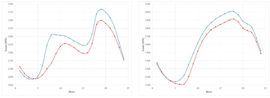
Figure 1.
The average of a 24-hour of load curve of weekdays (blue solid) and weekends (red dashed) 1993–2012 (left: January; right: July).
The weather variables, such as temperature, humidity, precipitation, and wind speed, have played a significant role in electricity load forecasting, such as in the models used by the PJM TRO. Out of these factors, the temperature plays a major role (Figure 2). The effect of seasons on the electricity load, as seen in Figure 3, can be mainly attributed to seasonal fluctuation of the temperature, even though seasonal changes in human behavior can also play a role. The proposed approach to modeling electricity load strives to capture these effects due to seasonality, week-day and weekend differences, as well as the intra-day fluctuation of temperature on the 24-hour load curve. Details of how this is accomplished are given in Section 4.
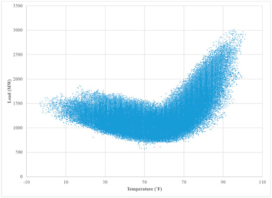
Figure 2.
The relationship between the hourly load and hourly temperature—South New Jersey 1993–2012.
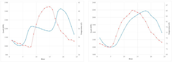
Figure 3.
The average of 24-hour load curves (blue solid) and the temperature (red doted) (left: January 2013; right: July 2013).
3. Data Sources
The historical load dataset used in this study was obtained from the Pennsylvania-New Jersey-Maryland RTO website (PJM) [24]. The data cover a sub region of PJM (see Figure 4), namely the Atlantic City Electric company (AE), which serve approximately 556,000 customers in eight counties (Atlantic, Burlington, Camden, Cape May, Cumberland, Gloucester, Ocean, and Salem), in southern New Jersey. This dataset includes hourly observations measured in megawatts (MW) over 20 years from 1 January 1993 through 31 December 2012 (see Figure 5), which were used for modeling purposes (i.e., as training data), and data from 1 January 2013 through 31 December 2013, shown in Figure 6, which were used as test data for computing forecasting error. The weather data were obtained from the National Oceanic Atmospheric Administration (NOAA) based on four weather stations in different locations of the study area, southern New Jersey. These stations are located in Atlantic City, Millville, Mount Holly, and Wildwood.

Figure 4.
Map of Pennsylvania-New Jersey-Maryland (PJM) [25].

Figure 5.
The hourly observed load over 20 years.
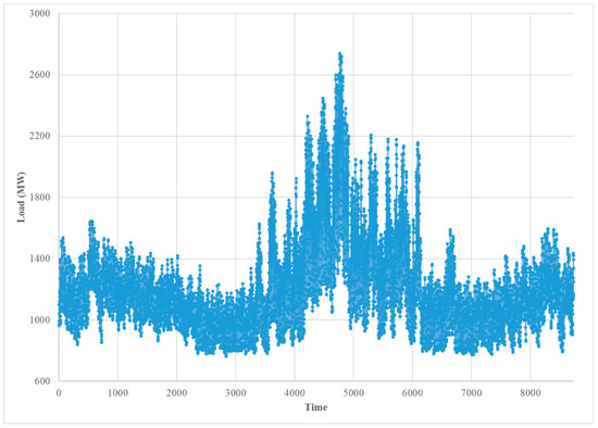
Figure 6.
The hourly load of Atlantic City Electric Company (AE) in 2013.
The economic data were obtained from Federal Reserve Bank of St. Louis. The specific economic variables used in this study are: industrial production index in the US (IPI) which is an economic indicator that measures the amount of the output from manufacturing, mining, electric and gas industries; government employment in New Jersey (NJGOVTN), which is defined as the total body of employees in all government agencies apart from the military; home vacancy rate in New Jersey (NJHVAC), which is defined as the percentage of all available units in a rental property that are vacant or unoccupied at a particular time.
4. The Proposed Approach to Modeling Electricity Load
The approach used in the following assumes a traditional structural time series model with trend, seasonal, and cyclical components, but utilizes a variation of cubic splines to estimate the 24-hour load profile for weekdays and weekends in a given season with hourly temperature playing an explanatory role. Specifically, model parameters are estimated for the mean load curve separately for weekdays and weekend days within each season after performing a de-trending operation. This approach can be considered suitable for short term prediction because of the need to have good estimates of hourly temperature.
The model assumes that , the real-time load at hour i on day t, is a composite of structural components consisting of a long-term trend , a seasonal component , a weekly cycle , a set of functions representing the hourly load profile at time x for season s and day of the week d (taking one value for week-days and a different value for weekends), and an irregular stochastic component . Thus, can be expressed as:
where t = 1, 2, …, N and i = 1, 2, …, 24. Note that N denotes the number of days in the training data set and i denotes the hour of the day.
The long-term trend was modeled using classical regression with select economic variables as regressors. The weakly seasonal component was modeled using a vector autoregressive moving average with exogenous terms (ARMAX) formulation with the average weekly temperature and its square as exogenous variables. The 24-hour load profiles were modeled by using a separate set of cubic splines for each season and weekdays/weekend combinations. Different spline models were used for each season because the 24-hour load profile within a season has almost the same pattern but differs across seasons. The weekdays were modeled separately within each season because they have quite different load profiles as well when compared to weekend patterns. The assumption of only one functional form for the load profile of weekdays can be relaxed by adding unique functions for each day of the week or for Monday, Friday, and the rest of the weekdays. Similarly, one can assume separate functional forms for Saturday and Sundays. Since such an approach can reduce the accuracy of estimates due to reduced sample sizes, the number of different functions was kept to a minimum.
Details of the modeling process are described below, beginning with the detrending process followed by the estimation of the seasonal components and concluding with the spline modeling of the 24-hour load profile.
4.1. Predicting Long-Term Trend
The first step included modeling the hourly average electricity load per year, , using classical regression analysis. Note that in the above expression for the average load, denotes the year with and denotes the total number of days in that year. A stepwise selection method was used to determine the independent variables to be included in the model. Out of more than 20 economic variables plus population size and the average monthly temperature, the following variables were selected: government employment in New Jersey (NJGOVTN), industrial production index in the US (IPI), home vacancy rate in New Jersey (NJHVAC), and the average temperature of September (Temp_Sep). Table 1 provides the results of the multiple linear regression analysis.

Table 1.
The results for the regression model for annual load.
The estimated regression model for the annual data is:
The selected independent variables explain 98.5% of the variation in the average annual load and the root mean square error (RMSE) is 9.7, which is relatively small. Moreover, no serious multicollinearity among the independent variables was detected. The residual analysis is shown in the Figure A1 in the Appendix A, and while two outliers (with high Cook’s distance) are shown, no major concern is raised. In addition, the model does a good job of predicting the annual load, as seen in Figure 7.
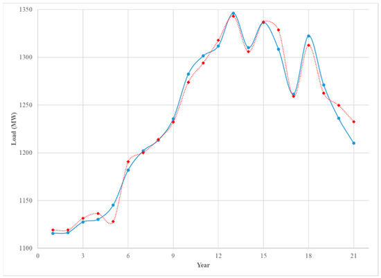
Figure 7.
The annual average of hourly load (blue solid) and the predicted load (red doted) 1993–2013.
Figure 7 displays the average annual real-time load per hour for the 20 years of training data and one year of test data and the average annual load predicted, using the estimated regression model. The figure shows the predicted trend using actual macroeconomic data for the test year, but the macroeconomic data for the test year can be predicted very accurately using an ARMA model, and the results do not change by much. The display shows very good in-sample agreement between the observed and predicted load and a reasonable agreement between the two for the test year. One word of caution is that we observed that the electricity load decreased in the last three years, but one of the two most important variables in the model, the government employment in New Jersey (NJGOVTN), decreased only slightly, while the industrial production index in the US (IPI) increased. Those two variables explained 92% of the variation in the electricity load. Thus, some delinking of these variables with electricity load may be occurring and developing an annual model with more recent data may be pragmatic.
4.2. Estimating Seasonal Variation in Data
The trend estimates for each year were transposed onto a weekly series, and a 52-week moving average was applied to this series to smooth the predictions from a step function to a smooth one. The smoothed trend, , for week w, was subtracted from the average load for each day within the corresponding week, with the process repeated for all weeks, yielding the detrended daily averages . The resulting data can be represented in a vector series , where each vector contains the seven detrended daily averages corresponding to that week. Note that w = 1, 2, …, W, where W is the total number of weeks in the training data set. The de-trended weekly time series, , was then used to fit a subset ARMAX model (see Baillie, R. T [26] for details) given below:
where denotes the autoregressive lag term, denotes the moving average lag terms, and T denotes the weekly average temperature. The residuals of the fit do not show any major autocorrelations and the test for white noise (bottom right hand corner of Figure A2 in the Appendix A) shows no evidence that the residuals are anything other than white noise. The check for normality of the residuals, given in Figure A3 in the Appendix A, shows some deviation from normality, but this is not much of a concern because the model performed an adequate job of extracting the seasonal component as indicated by white noise residual.
The forecasted weekly vector values for the test data set (year 2013) were then obtained using the estimated ARMAX model. These estimated vectors contain forecasted daily values for each week. These daily values were averaged to get a forecast weekly average. The trend model was then employed to forecast a yearly trend for the test data (year 2013). Note that to predict a trend, we needed macroeconomic data for the test year and in practice, these have to be predicted. We found that applying an ARMA model to the past macroeconomic data would yield accurate forecasts for the test year. This yielded a constant forecast across all the weeks of the test year. These were them smoothed using a 52-week moving average that utilized previous year’s data for the smoothing. The smoothed weekly trend data were then added to the forecast weekly average obtained from averaging the daily values from the ARMAX vector forecasts. The resulting weekly averages were then compared with the observed weekly average load for the test year (Figure 8). These out-of-sample checks show that the seasonal (weekly) model provides a satisfactory estimation of the seasonal component.
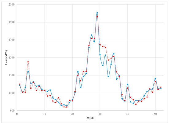
Figure 8.
The weekly average of the hourly load (blue solid) and the predicted load (red dashed) in 2013.
Note that the smoothing of the yearly trend data allows for a smooth transition from one year to the next. It also reduces any bias due to poor estimation of the trend value for the test year, when computing trend values for the early part of the test year. The trend estimates can be updated later in the test year by reforecasting the trend value by using updated macroeconomic variables that may become available after the first quarter of that year and later after the second and third quarter.
4.3. Modeling the Hourly Load
At this point, the weekly smoothed trend and the estimated seasonal component were removed from the hourly data for both training and test data years, and a new de-trended and de-seasonalized time series, , was obtained. The times series was modeled using the training data set, by fitting cubic splines to model the 24-hour daily profile. Different spline estimates were obtained for each season, weekday, and weekend combination. Temperature and its interaction with time were also fitted as regressors.
Two scenarios were applied here. The first one modeled each season and each day type (weekday or weekend) separately. We denoted the resulting model as Model 1. The second scenario modeled each season separately and ignored the day type but added a dummy variable to identify the type of day. This approach provided us with Model 2.
4.3.1. The First Scenario
The general spline Model 1 is:
where i is the hour, are the knots that change according to season and day type, and is temperature at hour i on day t. The knot positions were chosen by inspection for each season and are given, together with the parameter estimates, in the Table A2, Table A3, Table A4 and Table A5 in the Appendix A. Note that non-significant terms were dropped from the model and what is given above is the reduced model.
4.3.2. The Second Scenario
The general spline Model 2 is:
where i is the hour, is a knot that changes according to the season and the knot positions and parameter estimates are given in the Table A6 and Table A7 in the Appendix A. Note that is the temperature at time i on day t, and wt is a dummy variable denoting weekend day. Note that non-significant terms were dropped from the model and the results reported are for the reduced model.
As mentioned previously, the Table A2 through Table A7, given in the Appendix A, present the knot positions and the results of the regression model for each season and each type of day. The tables for weekdays and weekends for a given season are paired together for easy comparison.
Model obtained for each season is different from the others, reflecting changes in the daily load profiles across seasons. The comparison between Model 1 and Model 2, based on Akaike Information Criteria (AIC) and Root Mean Square Error (RMSE) is presented in Table 2. The results show very little difference between the two models. In addition, the Figures 10 and 11 show the comparison between the two models based on the Coefficient of Variation (CV) for each month and each hour, respectively.
Table 2.
The comparison between the two models.
Figure 9 shows very close agreement between the two models when compared using the CV by month. There is a slight drop in the CV for Model 1 suggesting a slight gain in accuracy when the weekdays and weekends are modeled separately. Figure 10 given below shows the CV for the two models by each hour of the day. Again, Model 1 shows a slight advantage with the CV for Model 2 showing higher values for hours before 10 am. This may be because the load profile for weekends shows a two-hour shift in the morning load profile and the inclusion of a dummy variable is not sufficient to account for this difference in the shape of the load profile.
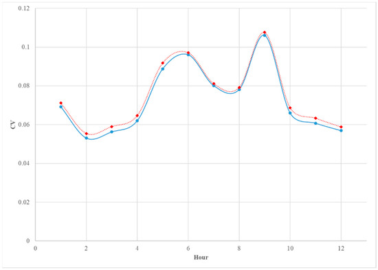
Figure 9.
The comparison between the CV of the predicted monthly average load of Model 1 (blue solid) and Model 2 (red doted).
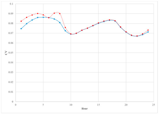
Figure 10.
The comparison between the CV of the predicted hourly average load of Model 1 (blue solid) and Model 2 (red doted).
The Figure 11, Figure 12, Figure 13 and Figure 14 provide a comparison between the two models for four different weeks of the test year. The weeks were chosen from the middle of each season. The forecasts based on each model were very close to one another, which suggests that adding a dummy variable for the day type instead of building the extra models for the type of day provides satisfactory forecast overall; however, for all seasons except summer, Model 2 yielded forecasts that fall below the observed load during the weekends (last two days in the graph), especially in the morning period. However, except for the weekends, both models underestimated the afternoon peak in winter and spring. For the summer season (Figure 13), the afternoon peak was overestimated by both models on Fridays.
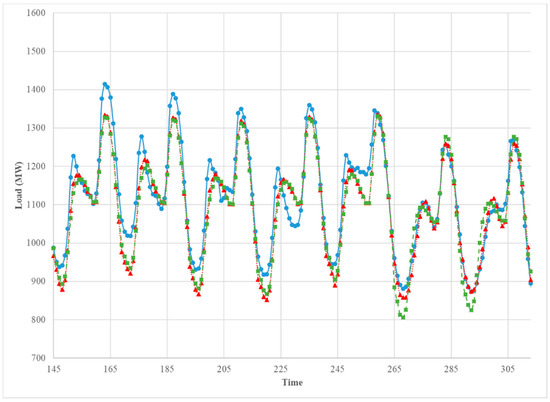
Figure 11.
The comparison between the observed hourly load (blue solid), the predicted hourly load of Model 1 (red doted), and Model 2 (green dashed). 7 January 2013–13 January 2013.
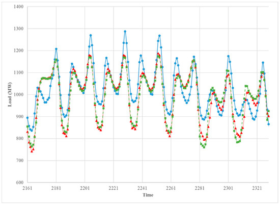
Figure 12.
The comparison between the observed hourly load (blue solid), the predicted hourly load of Model 1 (red doted), and Model 2 (green dashed). 1 April 2013–7 April 2013.
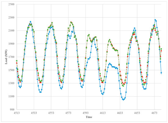
Figure 13.
The comparison between the observed hourly load (blue solid), the predicted hourly load of Model 1 (red doted), and Model 2 (green dashed). 8 July 2013–14 July 2013.
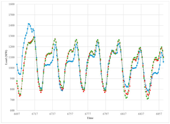
Figure 14.
The comparison between the observed hourly load (blue solid), the predicted hourly load of Model 1 (red doted), and Model 2 (green dashed). 7 October 2013–13 October 2013.
Table 3 provides an additional contrast between the two models based on CV. It is immediately apparent that any difference between the two models is quite marginal and may not have any practical consequences. The cells highlighted in light blue indicate places where the CV for a given model is lower than that for the competing model. If any conclusion can be made based examining these results, it may be that Model 1 is slightly better than Model 2 across most hours in winter and fall, and Model 1 appears to perform slightly better before noon during spring. One reason for this may be the somewhat poor performance of model two during the weekend mornings. If pressed to select one model over the other, the natural choice would be Model 1, but a strong argument cannot be made that it is much more superior to Model 2.
Table 3.
The comparison between the CV of the two models for each season by hour.
5. Conclusions
A multi-step approach to modeling the hourly electricity load using a structural time series model that utilizes only standard statistical modeling techniques was introduced. While the proposed methods require multiple steps to model the load data, every step can be implemented using commonly available statistical software packages, and therefore, they are within the reach of empirical modelers who do not have training in the use of sophisticated machine learning algorithms or have the time required to master complex analytical techniques. The results of modeling observed real-time load data from the PJM market show that the proposed method performs reasonably well in modeling the training data and short-term forecasting out-of-sample data. In addition, the proposed methodology utilized only macroeconomic and temperature data, and the use of additional input variables has the potential to further improve the performance of the models considered in this study. One shortcoming of the proposed study is the need to know macroeconomic data and the population figures to predict long-term trend, but in the context of forecasting in the short-term, this may not be a great drawback, because near-term forecasts of these can be quite reliable or one can use the most recent data without sacrificing much accuracy. In spite of the above shortcoming, it is seen that the cubic spline model worked very well in capturing the 24-hour load curve, and therefore, the proposed methodology can provide a framework for modeling other phenomena that exhibit a daily cycle, especially if long-term trend forecasting is not needed.
Author Contributions
The contributions made by the two authors are as follows: conceptualization, A.J. and V.A.S.; methodology, A.J. and V.A.S.; software, A.J.; validation, A.J.; formal analysis, A.J.; investigation, A.J.; resources, V.A.S.; data curation, A.J.; writing—original draft preparation, A.J.; writing—V.A.S.; visualization, A.J.; supervision, V.A.S.; project administration, V.A.S.
Funding
This research received no external funding.
Conflicts of Interest
The authors declare no conflict of interest.
Appendix A
In this appendix, additional figures and tables relevant to material presented in this paper are given.

Figure A1.
Residual Analysis of the Annual Regression Model.
Figure A1.
Residual Analysis of the Annual Regression Model.


Figure A2.
Analysis of Residual for the Weekly ARMAX Model.
Figure A2.
Analysis of Residual for the Weekly ARMAX Model.


Figure A3.
Normality Diagnostics of the Residuals of the Weekly ARMAX Model.
Figure A3.
Normality Diagnostics of the Residuals of the Weekly ARMAX Model.

Table A1.
The Results for the Weekly ARMAX Model.
Table A1.
The Results for the Weekly ARMAX Model.
| Maximum Likelihood Estimation | |||||
|---|---|---|---|---|---|
| Parameter | Estimate | Standard Error | t Value | Approx. Pr > |t| | Lag |
| MU | 1023.0 | 28.446 | 35.96 | <0.0001 | 0 |
| MA1,1 | 0.751 | 0.06 | 12.55 | <0.0001 | 1 |
| MA1,2 | −0.056 | 0.019 | −2.99 | 0.0028 | 50 |
| MA1,3 | 0.712 | 0.037 | 19.22 | <0.0001 | 52 |
| MA1,4 | −0.440 | 0.048 | −9.22 | <0.0001 | 53 |
| MA1,5 | −0.105 | 0.025 | −4.24 | <0.0001 | 54 |
| AR1,1 | 1.128 | 0.057 | 19.67 | <0.0001 | 1 |
| AR1,2 | −0.227 | 0.033 | −6.87 | <0.0001 | 2 |
| AR1,3 | 0.762 | 0.027 | 28.06 | <0.0001 | 52 |
| AR1,4 | −0.673 | 0.031 | −22.11 | <0.0001 | 53 |
| T | −50.357 | 0.958 | −52.56 | <0.0001 | 0 |
| T2 | 0.533 | 0.01 | 57.50 | <0.0001 | 0 |
| Constant Estimate | 10.074 | Std Error Estimate | 41.473 | ||
| AIC | 10765.4 | SBC | 10824.8 | ||
Table A2.
The Results for the Regression Model for the Winter Season (Model 1).
Table A2.
The Results for the Regression Model for the Winter Season (Model 1).
| Winter—Weekdays | Winter—Weekends | |||||
|---|---|---|---|---|---|---|
| Variable | Parameter Estimate | Pr > |t| | Variable | Parameter Estimate | Pr > |t| | |
| Intercept | −43.94700 | 0.0003 | Intercept | 33.16159 | 0.0438 | |
| i | 43.00126 | <0.0001 | i | −68.74540 | <0.0001 | |
| i2 | −28.47236 | <0.0001 | i2 | 10.86316 | 0.0456 | |
| i3 | 3.90525 | <0.0001 | i3 | −0.34335 | 0.5244 | |
| (i − 6)2 | −72.28854 | <0.0001 | (i − 5)2 | 4.53027 | 0.1994 | |
| (i − 14)2 | −42.29815 | <0.0001 | (i − 12)2 | 21.97808 | <0.0001 | |
| (i − 17)2 | −103.8987 | <0.0001 | (i − 17)2 | −42.63870 | <0.0001 | |
| (i − 6)3 | −1.95948 | <0.0001 | (i − 5)3 | −0.98781 | 0.0461 | |
| (i − 14)3 | 8.92152 | <0.0001 | (i − 12)3 | 2.63976 | <0.0001 | |
| (i − 17)3 | −9.58272 | <0.0001 | (i − 17)3 | −0.96957 | 0.0194 | |
| temp | −2.89175 | <0.0001 | temp | −2.59769 | <0.0001 | |
| T*i | −0.71365 | <0.0001 | T*i | −0.15635 | 0.0027 | |
| T* i2 | 0.17868 | <0.0001 | T* (i − 5)2 | 0.06344 | <0.0001 | |
| T* i3 | −0.01462 | <0.0001 | T*(i − 12)2 | −0.56360 | <0.0001 | |
| T* (i − 6)2 | 0.26047 | <0.0001 | T*(i − 17)2 | −0.67866 | 0.0005 | |
| T*(i − 14)2 | 0.23657 | <0.0001 | T*(i − 12)3 | 0.06180 | <0.0001 | |
| T*(i − 17)3 | 0.02458 | <0.0001 | T*(i − 17)3 | −0.03642 | 0.0005 | |
| RMSE | 72.961 | RMSE | 74.388 | |||
| Adj-R2 | 0.767 | Adj-R2 | 0.707 | |||
| AIC | 260089.07 | AIC | 100750.97 | |||
Table A3.
The Results for the Regression Model for the Spring Season (Model 1).
Table A3.
The Results for the Regression Model for the Spring Season (Model 1).
| Spring—Weekdays | Spring—Weekends | |||||
|---|---|---|---|---|---|---|
| Variable | Parameter Estimate | Pr > |t| | Variable | Parameter Estimate | Pr > |t| | |
| Intercept | 93.65097 | <0.0001 | Intercept | −7.13119 | 0.6187 | |
| i | −150.22285 | <0.0001 | i | −48.84602 | <0.0001 | |
| i2 | 68.15250 | <0.0001 | i2 | 13.06001 | <0.0001 | |
| i3 | −8.97118 | <0.0001 | i3 | −0.74388 | <0.0001 | |
| (i − 4)2 | 115.05545 | <0.0001 | (i − 9)2 | −13.54758 | 0.0001 | |
| (i − 8)2 | 61.51265 | <0.0001 | (i − 18)2 | 124.02630 | 0.0021 | |
| (i − 19)2 | −124.08785 | <0.0001 | (i − 20)2 | 231.54827 | 0.0011 | |
| (i − 4)3 | −3.47963 | 0.0009 | (i − 9)3 | 2.62643 | <0.0001 | |
| (i − 8)3 | 13.74708 | <0.0001 | (i − 18)3 | −66.42324 | <0.0001 | |
| (i − 19)3 | 9.48140 | <0.0001 | (i − 20)3 | 65.77067 | <0.0001 | |
| temp | −2.50879 | <0.0001 | Temp | −1.45289 | <0.0001 | |
| T* i2 | −0.41258 | <0.0001 | T* i2 | −0.22542 | <0.0001 | |
| T* i3 | 0.07054 | 0.0001 | T* i3 | 0.02324 | <0.0001 | |
| T* (i − 4)2 | −1.05263 | <0.0001 | T* (i − 9)2 | −0.43314 | <0.0001 | |
| T* (i − 8)2 | −1.02330 | <0.0001 | T*(i − 18)2 | −2.77329 | <0.0001 | |
| T*(i − 19)2 | 1.75668 | <0.0001 | T*(i − 20)2 | −5.14219 | <0.0001 | |
| T* (i − 4)3 | 0.06608 | <0.0001 | T*(i − 9)3 | −0.03102 | <0.0001 | |
| T* (i − 8)3 | −0.14706 | <0.0001 | T*(i − 18)3 | 1.26328 | <0.0001 | |
| T*(i − 19)3 | −0.19409 | <0.0001 | T*(i − 20)3 | −1.22318 | <0.0001 | |
| RMSE | 73.524 | RMSE | 84.087 | |||
| Adj-R2 | 0.75 | Adj-R2 | 0.625 | |||
| AIC | 271284.41 | AIC | 111701.59 | |||
Table A4.
The Results for the Regression Model for the Summer Season (Model 1).
Table A4.
The Results for the Regression Model for the Summer Season (Model 1).
| Summer—Weekdays | Summer—Weekends | |||||
|---|---|---|---|---|---|---|
| Variable | Parameter Estimate | Pr > |t| | Variable | Parameter Estimate | Pr > |t| | |
| Intercept | −1031.8216 | <0.0001 | Intercept | −1121.8108 | <0.0001 | |
| i | 20.83889 | 0.6311 | i | 92.24404 | 0.0765 | |
| i2 | 23.34519 | 0.0028 | i2 | −4.50357 | 0.5201 | |
| i3 | −2.15146 | <0.0001 | i3 | 0.23011 | 0.4594 | |
| (i − 9)2 | −58.35710 | <0.0001 | (i − 7)2 | −50.56548 | 0.0002 | |
| (i − 14)2 | −52.55395 | 0.0212 | (i − 12)2 | 79.89184 | <0.0001 | |
| (i − 19)2 | −55.43427 | 0.1113 | (i − 20)2 | −45.09066 | 0.0476 | |
| (i − 9)3 | 13.63412 | <0.0001 | (i − 7)3 | 0.75179 | 0.4427 | |
| (i − 14)3 | −10.04996 | <0.0001 | (i − 12)3 | −1.41147 | 0.3334 | |
| (i − 19)3 | −3.42800 | <0.0001 | (i − 20)3 | −5.65133 | <0.0001 | |
| temp | 12.30673 | <0.0001 | temp | 13.92763 | <0.0001 | |
| T*i | −1.67881 | 0.0056 | T*i | −2.61695 | <0.0001 | |
| T* i2 | −0.23403 | 0.0326 | T* i2 | 0.15085 | 0.0283 | |
| T* i3 | 0.03886 | <0.0001 | T* (i − 7)2 | 1.43653 | <0.0001 | |
| T*(i − 14)2 | 1.07409 | 0.0002 | T*(i − 20)2 | 0.72256 | 0.0058 | |
| T*(i − 19)2 | 1.20714 | 0.0053 | T*(i − 7)3 | −0.14516 | <0.0001 | |
| T*(i − 9)3 | −0.17607 | <0.0001 | T*(i − 12)3 | 0.15275 | <0.0001 | |
| T*(i − 14)3 | 0.09527 | <0.0001 | ||||
| RMSE | 121.682 | RMSE | 138.235 | |||
| Adj-R2 | 0.866 | Adj-R2 | 0.815 | |||
| AIC | 303082.91 | AIC | 124226.62 | |||
Table A5.
The Results for the Regression Model for the Fall Season (Model 1).
Table A5.
The Results for the Regression Model for the Fall Season (Model 1).
| Fall—Weekdays | Fall—Weekends | |||||
|---|---|---|---|---|---|---|
| Variable | Parameter Estimate | Pr > |t| | Variable | Parameter Estimate | Pr > |t| | |
| Intercept | −124.73508 | <0.0001 | Intercept | −21.40477 | 0.3987 | |
| i | 49.54582 | 0.0001 | h | −27.84008 | 0.0282 | |
| i2 | −20.69335 | <0.0001 | h2 | 7.44891 | 0.0016 | |
| i3 | 2.88465 | <0.0001 | h3 | −0.32170 | 0.0803 | |
| (i − 6)2 | −62.12202 | <0.0001 | (i − 8)2 | −14.30060 | 0.3538 | |
| (i − 15)2 | 106.77851 | <0.0001 | (i − 10)2 | 5.40145 | 0.5837 | |
| (i − 20)2 | 190.28792 | <0.0001 | (i − 18)2 | −147.68332 | <0.0001 | |
| (i − 6)3 | −1.41533 | <0.0001 | (i − 8)3 | −1.67366 | 0.6195 | |
| (i − 15)3 | −17.40696 | <0.0001 | (i − 10)3 | 5.28608 | 0.1368 | |
| (i − 20)3 | 4.95084 | <0.0001 | (i − 18)3 | 5.18245 | <0.0001 | |
| temp | −0.55227 | 0.0901 | temp | −1.22595 | 0.0026 | |
| T* i | −0.95896 | <0.0001 | T* i | −0.87935 | <0.0001 | |
| T* i2 | 0.05788 | 0.0049 | T* i2 | 0.00681 | <0.0001 | |
| T* (i − 6)2 | 0.31932 | <0.0001 | T* (i − 8)2 | 0.68040 | 0.0036 | |
| T*(i − 15)2 | −1.29167 | <0.0001 | T*(i − 18)2 | 1.72536 | <0.0001 | |
| T*(i − 20)2 | −3.25219 | <0.0001 | T*(i − 8)3 | −0.14824 | 0.0002 | |
| T* (i − 6)3 | −0.02245 | <0.0001 | T*(i − 10)3 | 0.11613 | 0.0105 | |
| T*(i − 15)3 | 0.23814 | <0.0001 | T*(i − 18)3 | −0.10069 | <0.0001 | |
| RMSE | 92.402 | RMSE | 100.78 | |||
| Adj-R2 | 0.745 | Adj-R2 | 0.653 | |||
| AIC | 282449.54 | AIC | 115156.88 | |||
Table A6.
The Results for the Regression Model for the Winter and Spring Seasons (Model 2).
Table A6.
The Results for the Regression Model for the Winter and Spring Seasons (Model 2).
| Winter | Spring | |||||
|---|---|---|---|---|---|---|
| Variable | Parameter Estimate | Pr > |t| | Variable | Parameter Estimate | Pr > |t| | |
| Intercept | −16.55248 | 0.1207 | Intercept | −28.71512 | 0.3281 | |
| i | 23.25116 | 0.0014 | i | 43.44180 | 0.1746 | |
| i2 | −20.66445 | <0.0001 | i2 | −18.69310 | 0.0568 | |
| i3 | 2.96367 | <0.0001 | i3 | 2.56499 | 0.0042 | |
| (i − 6)2 | −52.98180 | <0.0001 | (i − 5)2 | 17.48659 | <0.0001 | |
| (i − 15)2 | −16.66555 | <0.0001 | (i − 8)2 | 42.40157 | <0.0001 | |
| (i − 17)2 | −112.22096 | <0.0001 | (i − 19)2 | −123.9761 | <0.0001 | |
| (i − 6)3 | −1.83272 | <0.0001 | (i − 5)3 | −13.11806 | <0.0001 | |
| (i − 15)3 | 13.03173 | <0.0001 | (i − 8)3 | 11.98398 | <0.0001 | |
| (i − 17)3 | −12.65773 | <0.0001 | (i − 19)3 | 9.16725 | <0.0001 | |
| temp | −2.76643 | <0.0001 | temp | −0.64997 | 0.2414 | |
| T* i | −0.64320 | <0.0001 | T* i | −2.15721 | 0.0003 | |
| T* i2 | 0.13092 | <0.0001 | T* i2 | 0.50905 | 0.0049 | |
| T* i3 | −0.00834 | <0.0001 | T* i3 | −0.04807 | 0.0027 | |
| T*(i − 6)2 | 0.12037 | 0.0070 | T*(i − 8)2 | −0.96311 | <0.0001 | |
| T*(i − 15)2 | 0.13705 | 0.0009 | T*(i − 19)2 | 1.72975 | <0.0001 | |
| T*(i − 17)3 | 0.01452 | <0.0001 | T* (i − 5)3 | 0.18007 | <0.0001 | |
| Weekend | −49.01851 | <0.0001 | T*(i − 8)3 | −0.14305 | <0.0001 | |
| T*(i − 19)3 | −0.18822 | <0.0001 | ||||
| Weekend | −59.90003 | <0.0001 | ||||
| RMSE | 75.781 | RMSE | 79.687 | |||
| Adj-R2 | 0.741 | Adj-R2 | 0.705 | |||
| AIC | 363556.63 | AIC | 386694.58 | |||
Table A7.
The Results for the Regression Model for the Summer and Fall Seasons (Model 2).
Table A7.
The Results for the Regression Model for the Summer and Fall Seasons (Model 2).
| Summer | Fall | |||||
|---|---|---|---|---|---|---|
| Variable | Parameter Estimate | Pr > |t| | Variable | Parameter Estimate | Pr > |t| | |
| Intercept | −1131.9170 | <0.0001 | Intercept | −84.22522 | <0.0001 | |
| i | 115.72585 | <0.0001 | i | 40.45021 | 0.0004 | |
| i2 | 1.12711 | 0.2755 | i2 | −17.21285 | <0.0001 | |
| i3 | −0.77157 | <0.0001 | i3 | 2.41275 | <0.0001 | |
| (i − 9)2 | −83.52495 | <0.0001 | (i − 6)2 | −51.38721 | <0.0001 | |
| (i − 14)2 | −46.86818 | 0.0578 | (i − 15)2 | 120.69047 | <0.0001 | |
| (i − 19)2 | −45.76871 | 0.1566 | (i − 20)2 | 205.64318 | <0.0001 | |
| (i − 9)3 | 13.02938 | <0.0001 | (i − 6)3 | −1.34485 | <0.0001 | |
| (i − 14)3 | −11.66866 | <0.0001 | (i − 15)3 | −18.15278 | <0.0001 | |
| (i − 19)3 | −3.20285 | <0.0001 | (i − 20)3 | 4.97629 | <0.0001 | |
| temp | 13.81380 | <0.0001 | temp | −0.70591 | 0.0145 | |
| T*i | −2.73699 | <0.0001 | T*i | −0.99218 | <0.0001 | |
| T* i3 | 0.02435 | <0.0001 | T* i2 | 0.06113 | 0.0008 | |
| T* (i − 9)2 | 0.30996 | 0.0564 | T* (i − 6)2 | 0.30423 | <0.0001 | |
| T*(i − 14)2 | 1.08035 | 0.0008 | T*(i − 15)2 | −1.37326 | <0.0001 | |
| T*(i − 19)2 | 1.11159 | 0.0059 | T*(i − 20)2 | −3.36051 | <0.0001 | |
| T*(i − 9)3 | −0.17592 | <0.0001 | T*(i − 6)3 | −0.02131 | <0.0001 | |
| T*(i − 14)3 | 0.11706 | <0.0001 | T*(i − 15)3 | 0.24565 | <0.0001 | |
| Weekend | −55.87929 | <0.0001 | Weekend | −71.82423 | <0.0001 | |
| RMSE | 128.175 | RMSE | 97.147 | |||
| Adj-R2 | 0.85 | Adj-R2 | 0.717 | |||
| AIC | 428670.67 | AIC | 399798.26 | |||
References
- Bunn, D.; Farmer, E. Comparative Models for Electrical Load Forecasting; John Wiley & Sons: New York, NY, USA, 1985. [Google Scholar]
- Alfares, H.; Nazeeruddin, M. Electric load forecasting: Literature survey and classification of methods. Int. J. Syst. Sci. 2002, 33, 23–34. [Google Scholar] [CrossRef]
- El-Keib, A.A.; Ma, X.; Ma, H. Advancement of statistical based modeling techniques for short-term load forecasting. Electr. Power Syst. Res. 1995, 35, 51–58. [Google Scholar] [CrossRef]
- Dash, P.K.; Liew, A.C.; Rahman, S. A comparison fuzzy neural network for the generation of daily average and peak load profiles. Int. J. Syst. Sci. 1995, 26, 2091–2106. [Google Scholar] [CrossRef]
- Kim, K.H.; Park, J.K.; Hwang, K.J.; Kim, S.H. Implementation of hybrid short-term load forecasting system using artificial neural networks and fuzzy expert system. IEEE Trans. Power Syst. 1995, 10, 1534–1539. [Google Scholar]
- Cho, H.; Goude, Y.; Brossat, X.; Yao, Q. Modeling and forecasting daily electricity load curves: A hybrid approach. J. Am. Stat. Assoc. 2013, 108, 7–21. [Google Scholar] [CrossRef]
- Choueiki, M.H.; Mount-Campell, C.A.; Ahalt, S. Implementing a weighted least squares procedure in training a neural network to solve the short-term load forecasting problem. IEEE Trans. Power Syst. 1997, 12, 1689–1694. [Google Scholar] [CrossRef]
- Gajowniczek, K.; Zabkowski, T. Two-stage electricity demand modeling using machine learning algorithms. Energies 2017, 10, 1–25. [Google Scholar]
- Das, S.P.; Laharika, V.; Achray, N.S. Improved short-term electricity load forecasting using extreme learning machine. In Proceedings of the International Conference on Big Data Analytics and Computational Intelligence (ICBDAC), Chirala, India, 23–25 March 2017. [Google Scholar]
- Annamareddi, S.; Gopinathan, S.; Dora, B. A simple hybrid model for short-term load forecasting. J. Eng. 2013, 5, 23–34. [Google Scholar] [CrossRef]
- Baziar, A.; Kavousi-Fard, A. Short term load forecasting using a hybrid model based on support vector regression. Int. J. Sci. Technol. Res. 2015, 4, 189–195. [Google Scholar]
- Nowicka-Zagrajek, J.; Weron, R. Modeling electricity loads in California: ARMA models with hyperbolic noise. Signal Process. 2002, 82, 1903–1915. [Google Scholar] [CrossRef]
- Liu, J.M.; Chen, R.; Liu, L.; Harris, J. A semi-parametric time series approach in modeling hourly electricity loads. J. Forecast. 2006, 25, 537–559. [Google Scholar] [CrossRef]
- Amaral, L.F.; Souza, R.C.; Stevenson, M. A smooth transition periodic autoregressive (ATPAR) model for short-term load forecasting. Int. J. Forecast. 2008, 24, 603–615. [Google Scholar] [CrossRef]
- Dordonnat, V.; Koopman, S.J.; Ooms, M.; Dessertaine, A.; Collet, J. An hourly periodic state space model for modeling French national electricity load. Int. J. Forecast. 2008, 24, 566–587. [Google Scholar] [CrossRef]
- Chapagain, K.; Kittipiyakul, S. Short-term electricity load forecasting model and Bayesian estimation for Thailand data. MATEC Web Conf. 2016, 55, 06003. Available online: https://www.matec-conferences.org/articles/matecconf/abs/2016/18/matecconf_acpee2016_06003/matecconf_acpee2016_06003.html (accessed on 1 November 2019). [CrossRef]
- Kosiorowski, D. Functional regression in short-term prediction of economic time series. Stat. Transit. 2014, 15, 611–626. [Google Scholar]
- Hyndman, R.J.; Shang, H.L. Functional time series forecasting. J. Korean Stat. Soc. 2009, 38, 199–211. [Google Scholar] [CrossRef]
- Papadopoulos, S.; Karakatsanis, I. Short term electricity load forecasting using time series and ensemble learning methods. In Proceedings of the IEEE Power and Energy Conference at Illinois (PECI), Champaign, IL, USA, 20–21 February 2015; ISBN 978-1-4799-7949-3. [Google Scholar]
- Alkhathami, M. Introduction to electric load forecasting methods. J. Adv. Electr. Comput. Eng. 2015, 2, 1–12. [Google Scholar]
- Yang, A.; Li, W.; Yang, X. Short-term electricity load forecasting based on feature selection and least squares support vector machines. Knowl. Based Syst. 2019, 163, 159–173. [Google Scholar] [CrossRef]
- PJM. PJM Manual 19. Load Forecasting and Analysis; PJM: Audubon, PA, USA, 2018. [Google Scholar]
- Fahad, M.U.; Arabab, N. Factor affecting short term load forecasting. J. Clean Energy Technol. 2014, 2, 305–309. [Google Scholar] [CrossRef]
- PJM. Historical Load Data. Available online: http://www.pjm.com/markets-and-operations/ops-analysis/historical-load-data.aspx (accessed on 6 May 2014).
- Kunkel, C. Reforms Across PJM’s 13-State Market are Costly and Regressive. Institute for Energy Economics and Financial Analysis. Available online: http://ieefa.org/pjms-reform/ (accessed on 10 December 2018).
- Baillie, R.T. Predictions from ARMAX models. J. Econom. 1980, 12, 365–374. [Google Scholar] [CrossRef][Green Version]


© 2019 by the authors. Licensee MDPI, Basel, Switzerland. This article is an open access article distributed under the terms and conditions of the Creative Commons Attribution (CC BY) license (http://creativecommons.org/licenses/by/4.0/).