Multi-Objective Based Optimal Energy Management of Grid-Connected Microgrid Considering Advanced Demand Response

Abstract

This paper proposes an optimal energy management approach for a grid-connected microgrid (MG) by considering the demand response (DR). The multi-objective optimization framework involves minimizing the operating cost and maximizing the utility benefit. The proposed approach combines confidence-based velocity-controlled particle swarm optimization (CVCPSO) (i.e., PSO with an added confidence term and modified inertia weight and acceleration parameters), with a fuzzy-clustering technique to find the best compromise operating solution for the MG operator. Furthermore, a confidence-based incentive DR (CBIDR) strategy was adopted, which pays different incentives in different periods to attract more DR participants during the peak period and thus ensure the reliability of the MG under the peak load. In addition, the peak load shaving factor (PLSF) was employed to show that the reliability of the peak load had improved. The applicability and effectiveness of the proposed approach were verified by conducting simulations at two different scales of MG test systems. The results confirm that the proposed approach not only enhances the MG system peak load reliability, but also facilitates economical operation with better performance in terms of solution quality and diversity.

1. Introduction

At present, power systems face major issues such as the intermittent supply of power sources due to the growing interest in renewable energy sources and energy storage systems as well as concerns regarding climate change. To this end, additional power plants can be constructed to support the network on the generation side [1], however, conventional generators involve high installation and operating costs due to the materials and transmission logistics as well as high pollutant emissions. To deal with the intermittent nature of renewable energies, researchers have proposed energy storage systems (ESSs) that can be charged or discharged by the system operator to preserve the power balance of the network [2]. Due to the high costs related to not only the system operating under suitable conditions, but also maintenance over a long service life, the integration of an energy storage system into a network may incur additional costs. Such technical and economic challenges as well as environmental concerns have inspired studies on a suitable scheme for system operators.

Demand-side management (DSM) [3] is a robust approach that regulates the demand of customers through various programs such as building upgrades, financial support, incentives, and behavioral changes via education. DSM can be classified into two types: energy efficiency and demand response (DR). Energy efficiency is usually considered as a perpetual load curtailment [4] whereas DR focuses on load elasticity, which can be considered as a temporary load reduction. In other words, DR encourages customers to reduce their power demand through certain incentive programs or education. DR can be further classified into price-based DR (PDR) and incentive-based DR (IDR). In PDR, consumer prices vary with the hours of operation in accordance with the supply-side cost; for example, prices are high, medium, and low for peak, off-peak, and low-peak periods, respectively [5]. IDR is a program in which participating consumers are awarded incentives according to the amount of power curtailed; this can be classified into four types: direct load control, load curtailment, demand bidding, and emergency demand reduction [6]. Recent years have witnessed an increase in the use of microgrids (MGs). Many researchers have employed MGs to test the DR performance in terms of how it can resolve the power supply uncertainty as well as economic and environmental problems [7,8,9]. A MG can be defined as a small-scale distribution network comprised of various renewable energy systems (RES) such as photovoltaic (PV) systems and wind turbines (WTs) as well as conventional generators such as thermal generators and diesel engines (DEs), energy storage systems (ESSs), and fuel cells. In general, it can be connected with the main grid to exchange power, or it can operate in an island mode in emergencies or remote locations [10].

Considerable effort has been devoted toward the energy management of a MG by adjusting the DR. In [11,12,13,14], significant effects in terms of reducing the operating cost by incorporating DR was fully analyzed. In [11], a genetic algorithm was adopted to show the effectiveness of the DR in reducing the operating cost of a MG. In [12], a hierarchical energy management system was proposed to deal with the uncertainty of renewable sources and loads for the optimal operation of a MG. In [13], a multi-agent system was used to optimize the operation of a MG including the DR strategy. In [14], the optimal operation of a multi-MG system incorporating DR was investigated. A dynamic DR program especially for customers was designed in [15,16] to maximize the benefits. In [15], a smart transactive energy framework for grid-connected multi-home MGs was proposed on the basis of the artificial bee colony algorithm. In [16], the optimal management of a hybrid MG was proposed by considering both PDR and the internal power market via the particle swarm optimization (PSO) algorithm. The DR strategy was considered to cope with the multi-objective problem by minimizing operating costs while maximizing the benefits, when optimizing energy management problem [17,18,19,20]. The multi-agent system was also employed in [17] to solve the economic dispatch problem with the DR by using the distributed constraint optimization scheme. In [18], a game-theory-based multi-objective dynamic economic dispatch problem was solved using an advanced interactive multi-dimensional modeling method. The economic dispatch problem was also addressed in [19], which considered the pollutant emissions, DR, and renewable energy sources by using the model predictive control algorithm. In [20], a stochastic multi-objective based optimal energy management considering DR was solved on the basis of the weighted sum technique with the fuzzy satisfying method. The authors in [21,22] demonstrated the effectiveness of DR in reducing both the operating cost and pollutant emissions. In [21], stochastic linear programming was used to solve the energy management problem with the presence of real time DR and a multiple power market. In [22], a multi-objective based energy management problem with DR was solved by the augmented epsilon constraint method.

The above-mentioned studies involving the DR strategy mainly focus on reducing the operating costs, pollutant emissions, and increasing the benefits. In this regard, the effectiveness of the DR scheme has been demonstrated through various methods. Although economic and environmental issues are significant aspects of MG operation, challenges related to the peak load should also be considered. By primarily reducing the peak period load, the MG operator can ensure the reliability of the MG in emergencies. Therefore, there is an evident need to alleviate the risk of the peak period load while ensuring economical and environmentally-friendly operation when considering the optimal energy management problem of a MG.

This study emphasized an optimal energy management approach with an advanced CBIDR strategy that was implemented to enhance the reliability of the MG by mainly decreasing the peak load. The validity of our proposed strategy was verified by comparing the PLSF value to quantify the benefits of our scheme. By incorporating CVCPSO with the fuzzy-clustering technique, the proposed approach becomes capable of finding the optimal operating solution of the MG.

The major contributions of this paper can be summarized as follows:

• The proposed optimal energy management implementing CBIDR could improve the reliability of the peak load when compared to the existing IDR strategy and increase the economic benefits of the MG, since the operating costs, utility benefit, and the stability of the peak load are effectively considered simultaneously. Therefore, the optimal operating solution for the MG is more reasonable and feasible.
• A peak load shaving factor (PLSF) was adopted to present the effectiveness of our proposed strategy in peak load curtailment. The proposed factor helps the MG operator to determine conditions when decision-making, during which DR strategy is more advantageous in peak load reduction and thus enhances the reliability.
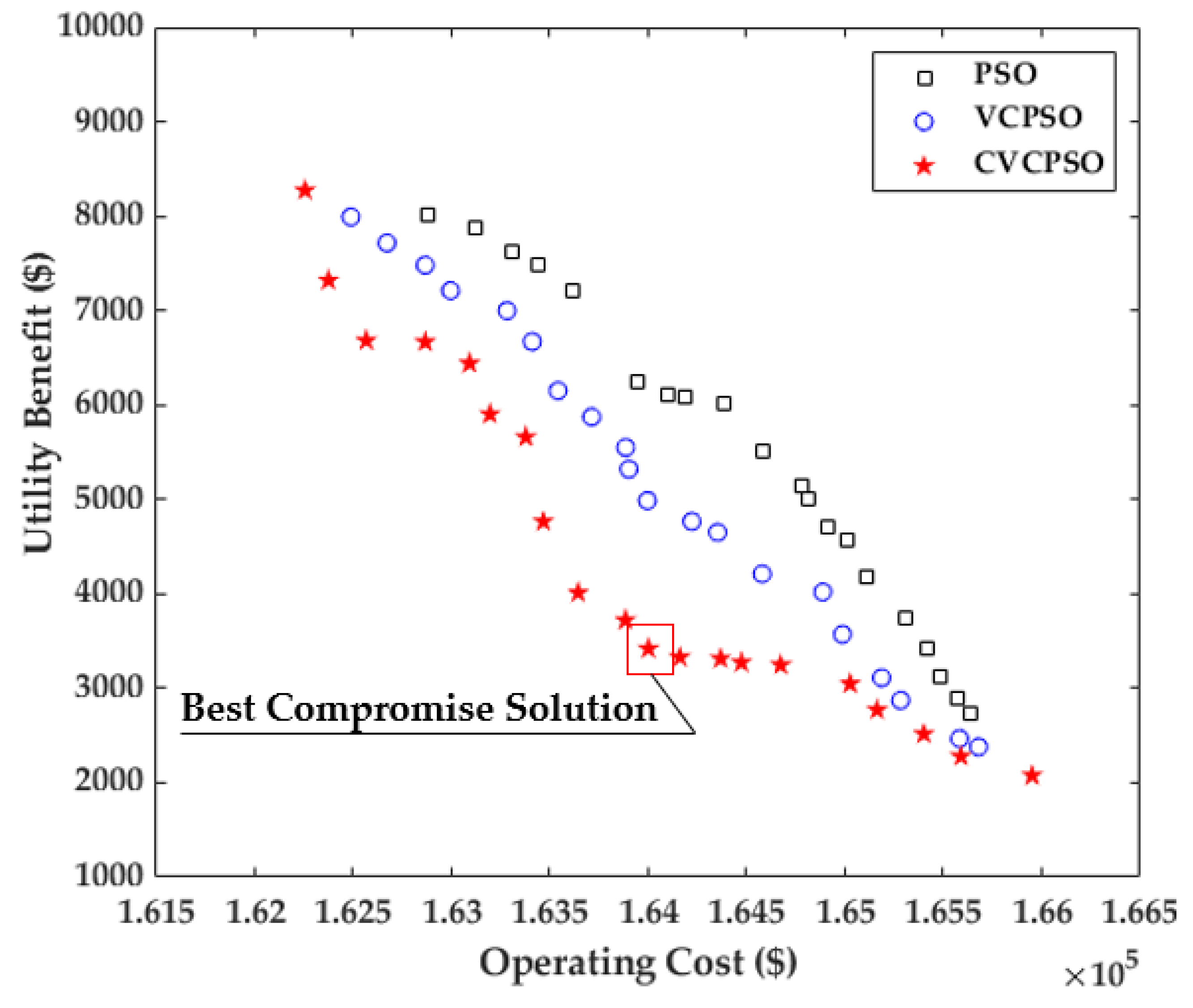
• A confidence-based velocity-controlled PSO (CVCPSO) with the recommended fuzzy-clustering technique was also formulated in the proposed approach for the MG system. By using CVCPSO, the solution quality and diversity of the optimal Pareto set was improved with respect to the conventional PSO and the best compromise solution can be obtained through the fuzzy-clustering technique.

Therefore, it was noted that the proposed approach presents an optimal energy management strategy with CBIDR for a grid-connected MG system in order to ensure the economic and reliable operation; in this regard, the proposed approach provides a more reasonable and flexible solution to the MG operator to consider the economic aspect and the risk of peak load simultaneously.

The remainder of this paper is organized as follows. Section 2 provides an overview of the grid-connected MG model. Section 3 introduces the proposed IDR strategy. Section 4 deals with the formulations of the multi-objective optimization problems. Section 5 describes the formulations of the CVCPSO algorithm and fuzzy-clustering technique. In addition, it summarizes the overall process of optimal energy management. Section 6 presents and analyzes the simulation results of the two different systems. Finally, Section 7 concludes the paper.

2. Overall Scheme of Grid-Connected Microgrid

2.1. Grid-Connected MG Model

The overall structure of the proposed grid-connected MG is shown in Figure 1 and consists of a photovoltaic (PV) system, wind turbine (WT), diesel engine (DE), and load. Clearly, most of the power sources considered in the MG are micro-power sources, in other words, the aggregation of small actual entities that cover various forms of power generation such as renewable energy generation (PV system and WT) and non-renewable generation (DE). To link the renewable and non-renewable energy, several power conversion systems could be requested by the MG [23]. Although converters can be synchronized with the grid to control the grid current and maximum power tracking point, the efficiency of the converter was not considered in our work because the DC/AC or DC/DC conversion efficiency is negligible in the MG system [24]. Moreover, in the MG system, various types of customers are assumed to be linked with an advanced metering infrastructure that provides the information required from the MG operator.

2.2. Modeling of WT

Wind power, an environment-friendly energy source, is the electric power generated by the rotation of turbine blades mounted on towers at a considerable height. As wind is probabilistic in nature, a WT has no control over its power generation. Thus, the power generated by a WT is solely dependent on the wind speed and tower height. Specifically, depending on the height at which the blades are mounted, wind speed can be converted from the anemometer height to the desired hub height in accordance with the following power law equation [25]:

$$\frac{v_2}{v_1}={(\frac{h_2}{h_1})}^{\alpha }$$

(1)

where α is the power law exponent defined by certain parameters (i.e., wind speed, terrain roughness, temperature, hour of day, height above ground, and time of year).

The value of α is generally considered as 0.11 and 0.2 for extreme and normal wind conditions, respectively [26]. The expected power output generated by the WT is expressed as

$$P_{WT}=\{\begin{array}{ccc}0& \mathrm{if}& v_{cut-off}\le v\le v_{cut-in}\\ P_r\times \frac{v^3-v^3{}_{cut-in}}{v^3-v^3{}_c}& \mathrm{if}& v_{cut-in}\le v\le v_{rated}\\ P_r& \mathrm{if}& v_{rated}\le v\le v_{cut-off}\end{array}$$

(2)

which is based on the rated power (P_r), rated speed (v), cut-in speed (v_cut-in), and cut-out speed (v_cut-out) of the WT.

2.3. Modeling of PV

Solar power is the electric power generated by PV panels from sunlight. The generated solar power can be calculated as follows [27]:

$$P_s={\eta }_s\times A\times SI(1+\beta (t_0-25))$$

(3)

The generated solar power depends on the efficiency (η_s) and size (A) of the PV panels as well as the solar irradiation (SI). Furthermore, β is generally denoted as a negative percentage per Kelvin or degree Celsius. The total output solar power (P_ST) can be calculated as

$$P_{ST}=N_S\times P_S$$

(4)

where N_S represents the number of solar generators.

2.4. Modeling of DE and Load

The DE is an important generator unit in the MG, which can be flexibly regulated by the MG operator. When the MG cannot satisfy the load through renewable energy generation, the DE operates as a secondary generation source to fulfill the load reliably. As the DE operates at a low loading rate with less efficiency, it should be controlled within a safe range to avoid unloaded and slightly loaded conditions.

Accurate modeling of the load is a prerequisite when solving the MG optimization problem. In general, the load is simply considered as the sum of individual customer units. However, here, we considered the load as individual customers who could be classified into different types depending on their willingness for DR engagement. In general, the customer type ranged from 0 to 1, where 0 denotes the least willing customer and 1 denotes the most willing customer for DR participation. In the following section, we propose a novel IDR scheme that considers various types of customer units.

3. Proposed Demand Response Strategy

We propose the CBIDR strategy to overcome the limitations of pre-determined IDR, which involves fixed incentive rates, and thus ensures system reliability under the peak load. To this end, the PLSF is used to quantify the specific benefits of implementing the CBIDR strategy.

3.1. Confidence-Based IDR

CBIDR primarily aims to encourage customers to reduce their load in the peak period through certain incentivizing strategies. Specifically, high incentives will be awarded when the load is in the peak period. In the CBIDR program, the value of the incentives awarded to the customers is considered as a function of the peak intensity (ρ), and it varies with the period in contrast to conventional IDR, which involves a fixed value. Accordingly, the incentive payment can be formulated as follows:

• Customer incentive

$$y_t={\rho }_t^{k-1}{x}_t^k={\rho }_t^{k-1}[D^k{}_t-D^{k-1}{}_t]$$

(5)

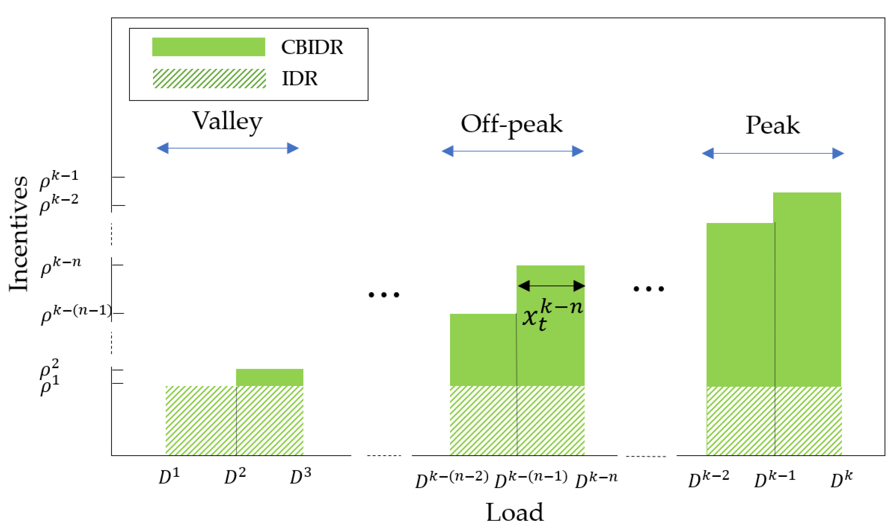
Here, ρ^k−1 is a function of the peak intensity, where higher incentives will be paid to the customer for load reduction during the peak period. Figure 2 compares the CBIDR and conventional IDR in terms of the incentive payment scheme. When the amount of load reduction is the same (D^k to D^k−1, D^k−n to D^k−(n−1), and D³ to D²) as x_t^k−n, the incentives (ρ^k−1, ρ^k−n, and ρ² for peak, off-peak, and valley period, respectively) paid to the customers vary with the period in which the DR event occurs. As shown in Figure 2, the incentive payment ρ^k−1 is higher for the same load reduction when compared with the off-peak and valley periods. This concept is an advantage of the CBIDR over the general IDR, where there is no such distinction between the incentive payments over the periods. It must be improved by considering incentive payments as a function of the peak intensity. This means that customers participating in the CBIDR program will earn higher incentive payments during the peak period than during the off-peak or valley periods. Higher incentives for peak reduction can motivate customers to take part in the DR program in the peak period. To this end, the customers must be more willing to decrease their load in the peak period with respect to the conventional IDR program.

• Customer cost function

$$c({\theta }_j,x_t^k)=K_1{(x_t^k)}^2+K_2{x}_t^k-K_2{x}_t^k{\theta }_j$$

(6)

Here, the −K₂x_t^kθ_j term is included to ensure that different values of θ_j leads to different values of customer marginal cost. Equation (6) represents the monetary loss incurred by load reduction x_t by a customer of type θ_j.

• Customer benefit function

$$B_{c,\text{\hspace{0.17em}}t}=y_t-c({\theta }_j,x_t)\text{\hspace{0.17em}}$$

(7)

Equation (7) defines the difference between the incentives and the cost incurred by the customer. The customer net benefit by load reduction x_t must be equal to or exceed zero in order to encourage DR action.

• Utility benefit function

$$B_{u,t}={\lambda }_t{x}_t-y_t$$

(8)

Equation (8) represents the total utility benefit for not supplying power to the customer for time t. During the peak period, it could be expensive to supply power to the customer. In other words, paying incentives to the customers in the peak period would be more cost-effective than supplying power to the customers. In this regard, introducing CBIDR is useful for reducing the peak load while increasing the grid reliability and reducing the supply cost.

• Load shedding constraints

$$D_t^{k,\min }\le x_t^k\le D_t^k,k=1$$

(9)

$$0\le x_t^k\le (D_t^k-D_t^{k-1}),k=2,3,...,K$$

(10)

$$x_{Total}={\displaystyle \sum _{k=1}^K{x}_t^k}$$

(11)

$$y_{j,t}^k-c({\theta }_j,x_t^k)\ge 0,j=1,2,...,J$$

(12)

$$y_{j,t}^k-c({\theta }_j,x_t^k)\ge y_{j,t}^{k-1}-c({\theta }_j,x_t^{k-1})k=2,...,K$$

(13)

Equation (9) implies that for k = 1, the load reduction should be less than D_t^k − D_t^k,min. Equation (10) represents a constraint for k = 2, 3, …, K, such that the load reduction in step k for time t must be less than D_t^k − D_t^k−1 and greater than zero. Equation (11) represents the total reduction for all the participants for time t. Equation (12) ensures that the customers’ net benefit exceeds zero. Equation (13) implies that the customers should be appropriately compensated for their load reduction.

3.2. Peak Load Shaving Factor

The main objective of implementing the CBIDR program is peak load shaving by paying higher incentives to the customers during the peak hours. To demonstrate the effectiveness of the CBIDR program, we propose the PLSF for the MG operator, which can be defined as

$$PLSF=\frac{APL{F}_W}{APL{F}_{WO}}$$

(14)

where APLF_W and APLF_WO denote the average to peak ratio (APLF) with and without DR, respectively. PLSF is the ratio between APLF_W and APLF_WO. This index represents the peak load reduction without DR. APLF can be defined as

$$APL{F}_W=\frac{1}{T}{\displaystyle \sum _{t=1}^T\frac{d_t^{\prime }}{d_{peak}^{\prime }}}\mathrm{and}APL{F}_{WO}=\frac{1}{T}{\displaystyle \sum _{t=1}^T\frac{d_t}{d_{peak}}}$$

(15)

APLF is defined as the ratio between the average load and the peak load in the same period. It represents the variability of the load, so that the higher the value of APLF, the greater the peak load shaving. If DR successfully curtails the load in the peak period, then APLF_W will increase and PLSF will improve accordingly. The higher the value of PLSF, the greater the enhancement of the system reliability during the peak period.

The PLSF quantifies the benefits of CBIDR unless d’_t reaches zero. It represents the effectiveness in terms of peak load reduction, which can be analyzed as follows:

• Condition 1. PLSF > 1.
• Condition 2. PLSF < 1.
• Condition 3. PLSF = 1.

In condition 1, when APLF_W is greater than APLF_WO, the value of PLSF will be greater than 1. This represents the amount of peak demand shaving achieved without DR.

In condition 2, when APLF_W is less than APLF_W, the value of PLSF is less than 1. This represents the reduction in APLF without DR.

In condition 3, PLSF = 1 (i.e., the APLF with and without DR are equal). This implies that the PLSF is constant.

The PLSF represents the quantitative results for various DR strategies, and the highest value among them is the best APLF with respect to the others. In addition, if all of the DR strategies achieve the same amount of load reduction, then the DR strategy with the higher PLSF value will be ranked higher in terms of the relative peak load reduction. Based on these values, the established indices can enable the MG operator to identify the DR benefits in terms of stability in the peak period.

4. Multi-Objective Optimal Formulation

The main objective of the optimal management of energy sources in the MG is to allocate the load among the available generation units economically and securely. To determine the optimal power generation units in the MG, a multi-objective optimization problem was solved by incorporating the CBIDR. The mathematical formulations of two different objectives subject to the related constraints are presented in the following subsection.

4.1. Objective Function

The MG multi-objective formulation consists of two objectives: (i) minimizing the operating cost function f₁(x), which includes the DE fuel cost, transaction cost, and pollutant treatment cost, by maximum use of renewable energies, and (ii) maximizing the utility benefit function f₂(x) by implementing DR.

4.1.1. Minimization of Operating Cost Function: f₁(x)

The objective function for minimizing the operating cost is as follows:

$$\min f_1(x)=\min \left({\displaystyle \sum _{t=1}^T{\displaystyle \sum _{z=1}^Z{F}_z(P_z(t))}}+{\displaystyle \sum _{t=1}^T{C}_{tr}({\mathrm{P}}_{tr}(t))}+{\displaystyle \sum _{t=1}^T{\displaystyle \sum _{z=1}^Z{C}_p(P_z(t))}}\right)$$

(16)

The DE fuel cost can be described as a quadratic model as follows:

$$F_z(P_z(t))=a_z{P}_z{(t)}^2+b_z{P}_z(t)$$

(17)

The transaction cost for trading transferable power between the main grid and the MG is given by

$$C_{tr}(P_{tr}(t))=\{\begin{array}{cc}{\gamma }_t\times P_{tr}(t)& \mathrm{Maingrid}\mathrm{to}\mathrm{MG}\\ 0& \mathrm{Disconnect}\\ -{\gamma }_t\times P_{tr}(t)& \mathrm{MG}\mathrm{to}\mathrm{main}\mathrm{grid}\end{array}$$

(18)

If the supply of the grid-connected MG cannot meet the demand, then power must be purchased from the main grid. In contrast, if the supply exceeds the demand, the power remaining after satisfying the demand can be sold to the main grid. In our study, locational marginal prices (LMPs) were used to obtain the power trading coefficient γ_t between the main grid and the MG [18].

The DE pollutant treatment cost [28] can be defined as

$$C_p(P_z(t))={\displaystyle \sum _e(C_e{\delta }_{z,e})\times P_z(t)}+{\displaystyle \sum _e(C_e{\delta }_{grid,e})\times P_{tr}(t)}$$

(19)

4.1.2. Maximization of Utility Benefit Function: f₂(x)

In this study, the IDR formulations (Equations (5)–(11)) were extended to more than a single time interval to incorporate them into the dynamic energy management problem. Equation (8) can be modified to adapt it to the total optimization problem horizon T instead of one time interval. Such conversion into a dynamic problem is more economical and practical in terms of solving the dynamic energy management problem. Finally, we adjusted the maximum power target for the utility benefit function f₂(x) as follows:

$$\max f_2(x)=\max \left({\displaystyle \sum _{t=1}^T{\displaystyle \sum _{j=1}^J{\displaystyle \sum _{k=1}^K{\lambda }_{j,t}{x}_{j,t}^k-y_{j,t}}}}\right)$$

(20)

where the number of customers is j over period T. Therefore, the MG operator makes a profit by not supplying power to certain customers and deducting incentive payments as shown in Equation (20).

4.2. Constraints

• Power balance constraints

$${\displaystyle \sum _{z=1}^Z{P}_z}+P_{WT}+P_{PV}+P_{tr}=D-{\displaystyle \sum _{j=1}^J{x}_j}$$

(21)

The total power generation from the DE, WT, and PV and transferred power from or to the main grid should match the load.

• Generation limit constraints for DE, WT, and PV

$$P_z^{\min }\le P_z\le P_z^{\max }$$

(22)

$$-D{R}_z\le P_{z,t+1}-P_{z,t}\le U{R}_z$$

(23)

$$0\le P_{WT}\le P_r$$

(24)

$$0\le P_{PV}\le P_{PV}{}^{\max }$$

(25)

Equation (22) represents the DE generation limit, which ensures that the generator is operated between the minimum and maximum power limits. Equation (23) denotes the increased or decreased DE power output per unit time t. Equations (24) and (25) represent the constraints of the minimum and maximum WT and PV generation limits, respectively.

• Transmission power constraints

$$-P_{tr}{}^{\max }\le P_{tr}\le P_{tr}{}^{\max }$$

(26)

Equation (26) represents the transmission power constraint, which ensures that the transmission power between the main grid and the MG does not exceed the maximum limit (P_tr^max).

• Demand response constraints

$${\displaystyle \sum _{t=1}^T\left({\rho }_{j,t}^k{x}_{j,t}^k-c(\theta ,x_{j,t}^k)\right)}\ge 0forj=1,...,J$$

(27)

$${\displaystyle \sum _{t=1}^T\left({\rho }_{j,t}^k{x}_{j,t}^k-c(\theta ,x_{j,t}^k)\right)}\ge {\displaystyle \sum _{t=1}^T\left({\rho }_{j,t}^{k-1}{x}_{j,t}^{k-1}-c(\theta ,x_{j,t}^{k-1})\right)}fork=2,...,K$$

(28)

$${\displaystyle \sum _{t=1}^T{\displaystyle \sum _{j=1}^J{y}_{j,t}\le UTDB}}$$

(29)

$${\displaystyle \sum _{t=1}^T{\displaystyle \sum _{k=1}^K{x}_{j,t}^k}}\le C{M}_j$$

(30)

Equations (27)–(30) represent the constraints of the utility benefit function f₂(x). Equations (27) and (28) can be substituted for Equations (12) and (13) over a day rather than a single time interval. Equation (27) ensures that a customer’s daily total incentives are greater than or equal to zero. Equation (28) implies that the greater the customers’ power consumption reduction, the greater the remuneration that they receive over the same period T. Equation (29) implies that the daily total incentives paid to the customer by the utility should be less than UTDB. Equation (30) ensures that the total daily power reduced by each customer does not exceed CM_j.

5. Solution Method

5.1. Confidence-Based Velocity-Controlled PSO

PSO is a population-based stochastic optimization technique inspired by bird flocking theory [29] and finds optimal solutions by attempting to improve a candidate solution iteratively. In a particle swarm optimizer, each particle denotes a potential solution to a problem, and it is regulated to search for the optimal solution by moving at a certain velocity in the search space in response to its own and its companions’ experience. The particles are treated in an N-dimensional space, and the ith particle, velocity, and position are expressed as X_i = (x_i1, x_i2, ⋯, x_iN), V_i = (v_i1, v_i2, ⋯, v_iN), and P_g = (p_g1, p_g2, ⋯, p_gN), respectively. The position and velocity of each particle will change according to the best and global positions. At each time step, the updated velocity and position of each particle is given by the following expression:

$$v_{i,n}(b+1)=w_1\times v_{i,n}(b)+c_1\times r_1\times (p_{best,i,n}(b)-x_{i,n}(b))+c_2\times r_2\times (g_{best,i,n}(b)-x_{i,n}(b))$$

(31)

$$x_{i,n}(b+1)=x_{i,n}(b)+v_{i,n}(b+1)$$

(32)

where c₁ and c₂ indicate the cognitive and social learning rates ranging from 0 to 1, respectively. In addition, r₁ and r₂ are random numbers ranging from 0 to 1, respectively.

The advantage of PSO lies in its simple principle and fast convergence. However, it tends to easily fall into local optima or converge prematurely. In a conventional PSO, there are three parameters (w₁, c₁, c₂) that are fixed. However, they should be adjusted several times to obtain the desired value. To overcome the limitations of a conventional PSO, we proposed the CVCPSO to improve the solution quality of the algorithm as follows [29,30]:

$$w_1=\frac{1}{2}\left(\cos \left({(m/M)}^l\pi \right)+1\right)$$

(33)

where l is a constant that varies according to the distribution of the population. Specifically, l = 0.5 or 2 when the distribution is too wide or too narrow, respectively; otherwise, l = 1. The inertia weight, w₁, is a critical constant that affects the convergence speed and performance of the algorithm. Therefore, the inertia weights should be set judiciously by considering a particle’s maximum movement distance to optimize its local and global exploration capabilities. In general, there is a trade-off between a particle’s search speed and its accuracy depending on the value of w₁. The higher the inertia weight, the higher the particle’s search speed and the lower its search accuracy. According to the characteristic of the inertia value, Equation (33) implies that, instead of being fixed, the inertia weight should vary with time, decreasing linearly or non-linearly, to achieve better performance. Therefore, given the characteristic of the inertia weight above-mentioned, Equation (33) can simultaneously guarantee high search accuracy and convergence speed.

In addition, if the particle velocities are not limited, then they may increase to unacceptable levels. Accordingly, the particle velocities should be regulated by introducing constriction coefficients c₁ (m) and c₂(m), given by

$$c_1(b)=(c_{1,final}-c_{1,initial})\frac{b}{B}+c_{1,initial}$$

(34)

$$c_2(b)=(c_{2,final}-c_{2,initial})\frac{b}{B}+c_{2,initial}$$

(35)

Equations (34) and (35) respectively ensure that c₁(m) decreases linearly and c₂(m) increases linearly to achieve the global search ability in the early stages of iteration and local optimization ability in the later stages of iteration. Here, c_1,initial, c_1,final, c_2,initial, and c_2,fianal are the initial and final values of c₁(m) and c₂(m), which were set to 2.5, 0.5, 0.5, and 2.5, respectively [31].

To avoid local optima and achieve global improvement, we added a confidence term by substituting the following equation into Equation (31):

$$v_{i,n}(b+1)=w_1\times v_{i,n}(b)+c_1\times r_1\times (p_{best,i,n}(b)-x_{i,n}(b))+c_2\times r_2\times (g_{best,i,n}(b)-x_{i,n}(b))-w_2{r}_3{g}_{best,i,n}(b)$$

(36)

Due to the effect of the confidence term, the velocity of the particles can be reduced at a certain iteration and the particle positions can be retreated in the opposite direction from the beginning accordingly. A particle’s retreating distance is assumed to be uncertain by employing the inertia weight w₂ and random variable r₃. Accordingly, the particle’s trust differs in each generation (i.e., the effect of g_best,i,n(b) varies). This improvement can reduce the density of the particles and thus maintain the particles’ diversity. To minimize the running time of the algorithm, we set w₁ = w₂.

5.2. Fuzzy-Clustering Technique

In general, multi-objective problems involve competing objectives. Non-commensurable and conflicting objectives that optimize more than two objective functions together cannot be solved by finding a single optimal solution. In this regard, acceptable solutions, rather than unit solutions, are attempted to be determined. To determine the superiority of solutions with respect to others, a concept of dominance is defined. Consider two vectors x₁ and x₂, where x₁ = [x_1,1, x_{1,2 ⋯}x_1,y], x₂ = [x_2,1, x_2,2⋯x_2,y], and y is the number of objective functions. In a maximization problem, a solution x₂ dominates x₁ if neither of the following two constraints is violated:

$$\forall p\in \{1,2,\cdots ,y\}:f_p(x_1)\le f_p(x_2)$$

(37)

$$\exists q\in \{1,2,\cdots ,y\}:f_q(x_1)\le f_q(x_2)$$

(38)

If all the above-mentioned constraints are satisfied, x₂ dominates x₁. A vector x₂ is called a non-dominated local set and the solutions that are non-dominated among the entire search space are called the non-dominated global set or the Pareto-optimal set. Accordingly, a multi-objective optimization problem leads to a set of optimal solutions called the Pareto-optimal set. In this study, a fuzzy-clustering technique [32] was used to extract the best solution that had the maximum value of the fuzzy membership function and provide it to the decision maker. The optimal-Pareto solution sets were converted into fuzzy membership functions as follows:

$${\mu }_y(a)=\frac{f_y{}^{\max }-f_y(a)}{f_y{}^{\max }-f_y{}^{\min }}$$

(39)

Finally, μ_y(a), considering all the objective functions, can be calculated as

$$\mu (a)=\frac{{\displaystyle {\sum }_{y=1}^S{w}_y{\mu }_y(a)}}{{\displaystyle {\sum }_{a=1}^U{\displaystyle {\sum }_{y=1}^S{w}_y{\mu }_y(a)}}}$$

(40)

The higher the value of μ(a), the higher the likelihood of obtaining the best compromise solution.

5.3. Solution Procedure

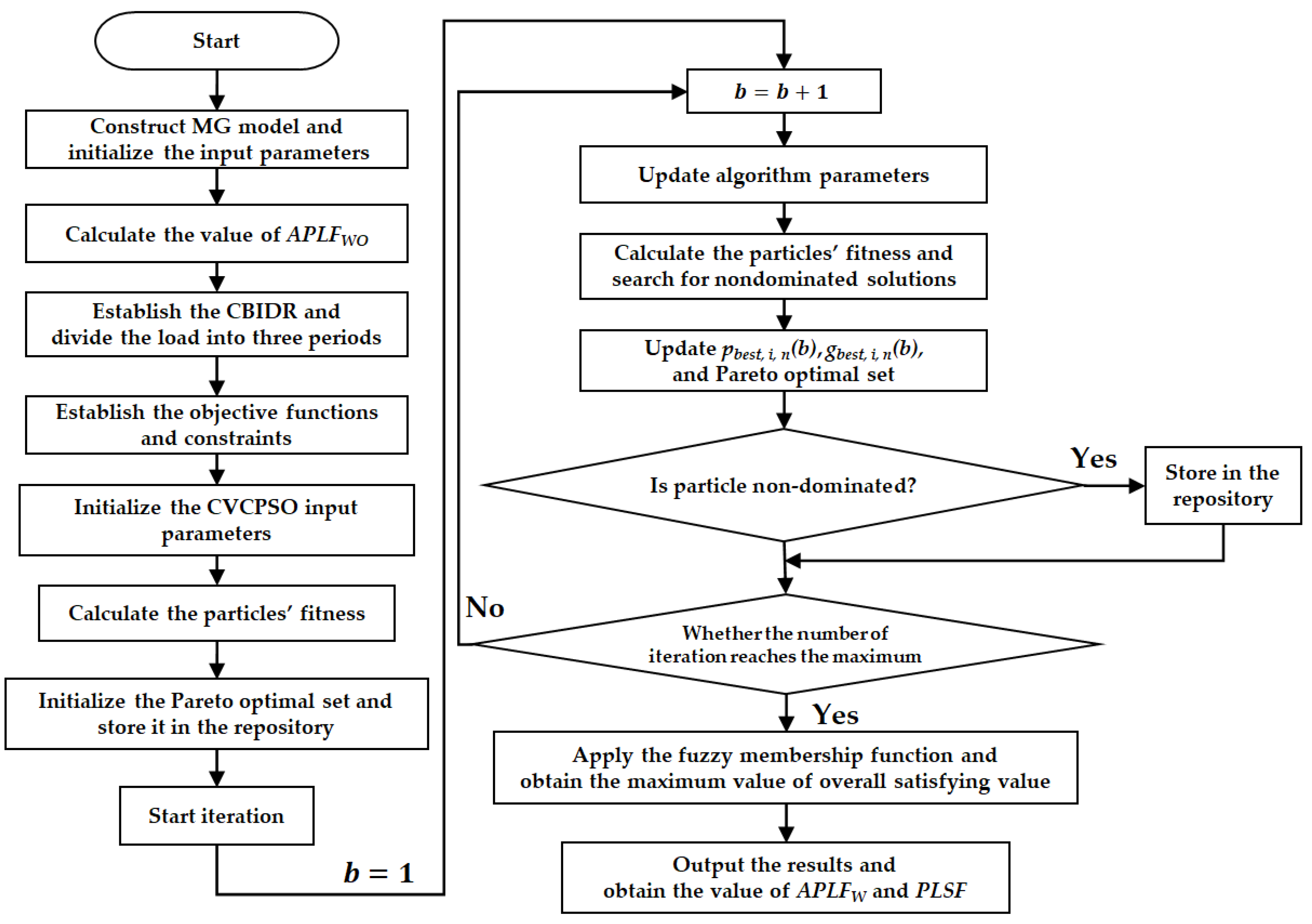
Optimal energy management procedure of the grid-connected MG implementing CBIDR is performed in the following sequential manner:

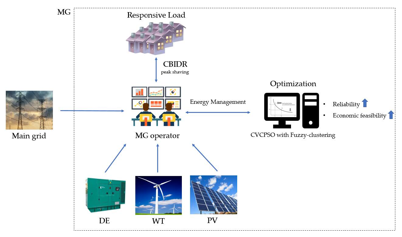
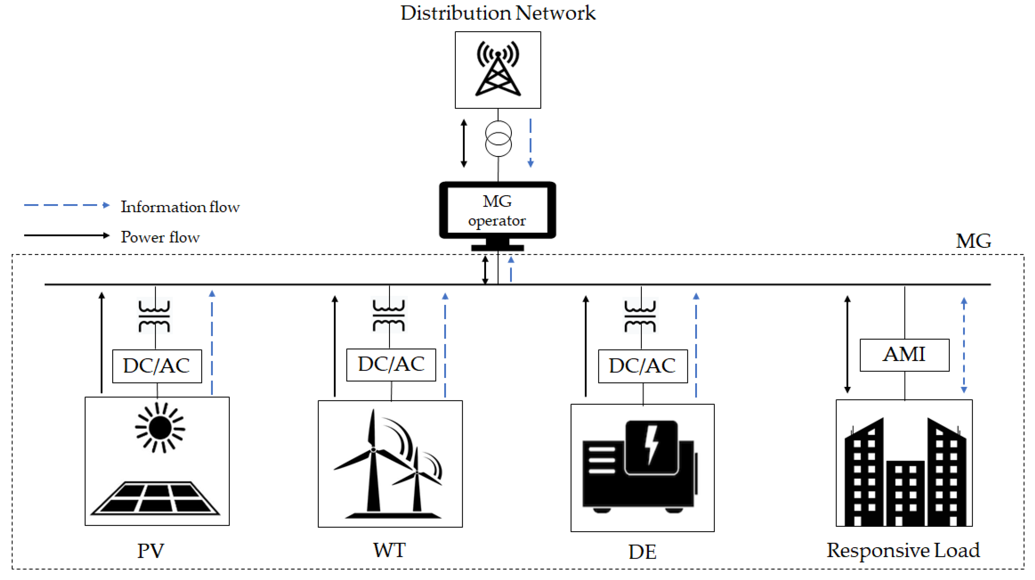
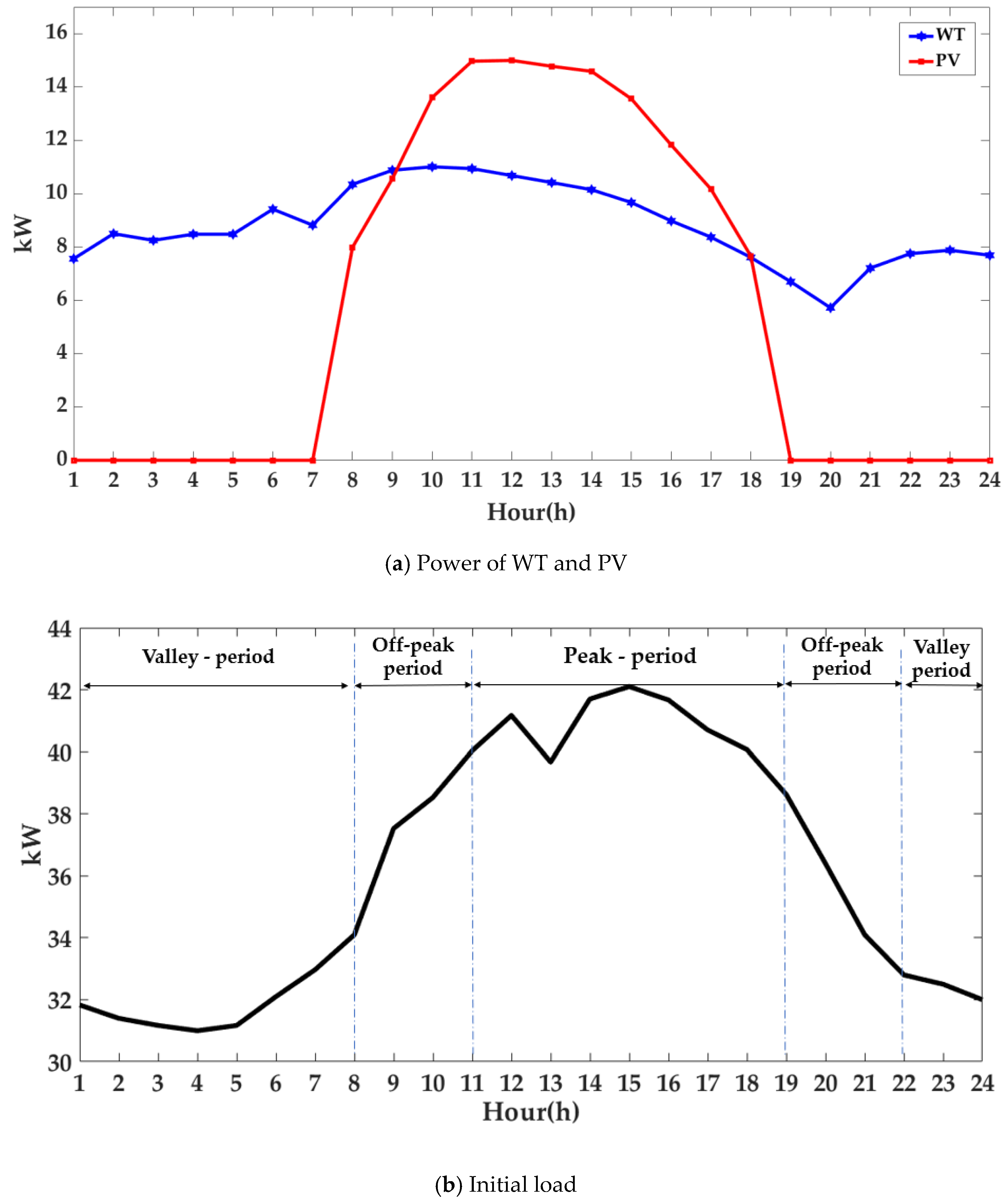
Step 1. Construct the MG model as shown in Figure 1 and initialize the MG input parameters (DE, WT, PV, and Load).

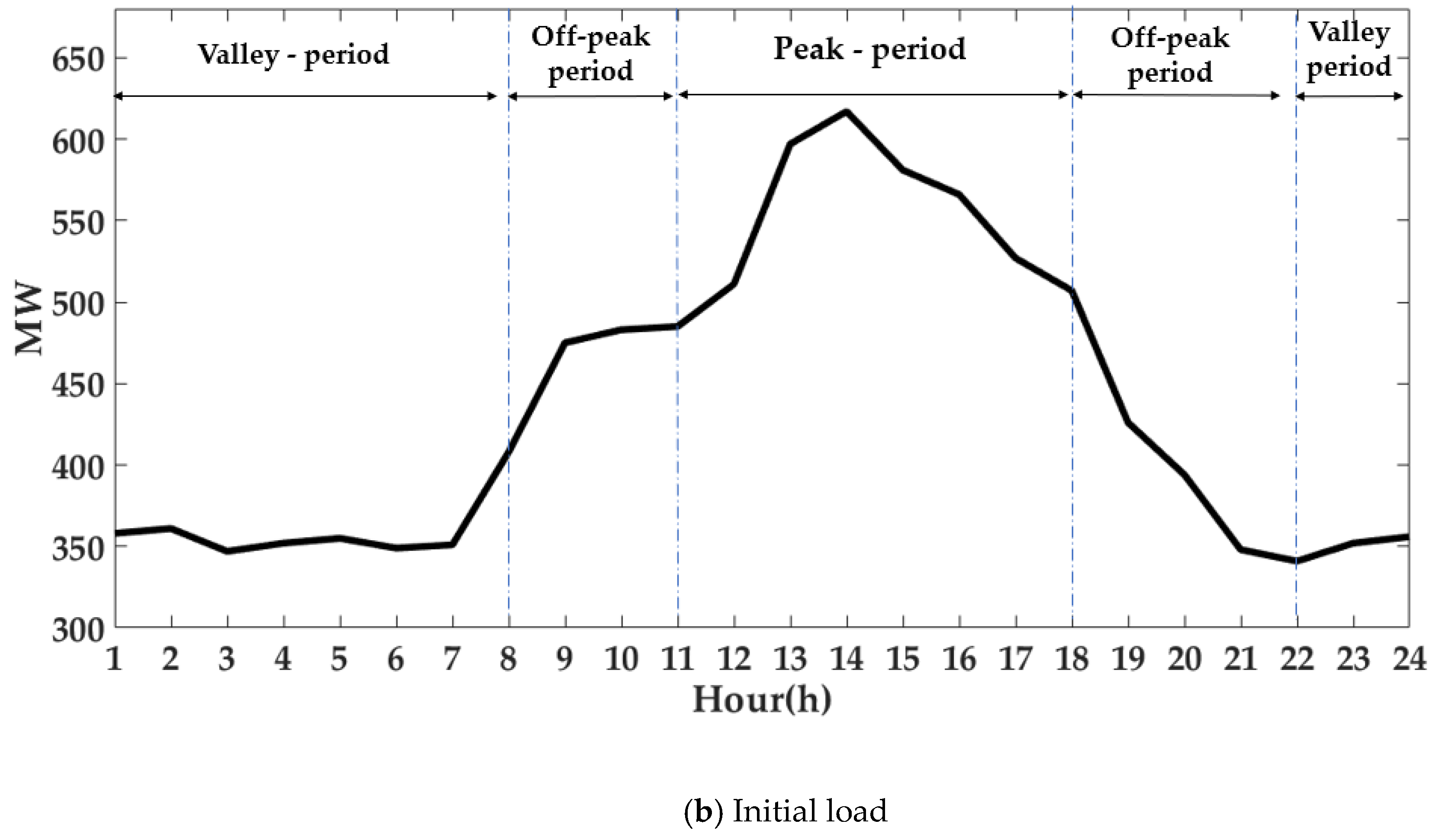
Step 2. Calculate the value of APLF_WO, according to Equation (15).

Step 3. Establish the CBIDR program as shown in Figure 2 and divide the load into three periods.

Step 4. Establish the objective functions and the corresponding constraints given by Equations (16)–(30). Set the CVCPSO input parameters (w₁, w₂, c₁(1), c₂(1), B, NP, S, and U) required to initialize the algorithm.

Step 5. Calculate the particle fitness according to the objective functions and the corresponding constraints. Initialize the Pareto-optimal set and store it in the repository.

Step 6. Start a loop iteration.

Step 7. Update the position and velocity of each particle according to Equations (32) and (36). Update the algorithm parameters w₁, w₂, c₁(m), and c₂(m) according to Equations (33)–(35).

Step 8. Calculate the particle fitness and update the non-dominated global set.

Step 9. Obtain the iteration results (i.e., the Pareto-optimal set) stored in the repository.

Step 10. Take the maximum value of the fuzzy membership function from Equation (39) and take the maximum value of μ(a) from Equation (40) to obtain the best compromise solution.

Step 11. Output the best compromise solution and calculate the values of APLF_W and PLSF.

The overall optimization process of MG energy management is shown in Figure 3.

6. Simulation Results

The validity and feasibility of the proposed approach were demonstrated using two MG test systems (1 and 2). First, we conducted a comparative analysis of two different IDR strategies: Case 1 (conventional IDR) and Case 2 (proposed CBIDR). The overall multi-objective optimization problems were solved using the CVCPSO algorithm, whose performance generally varies according to the size of the particles and the number of iterations. The number of particles and maximum number of iterations were set to 20,000 and 100, respectively, for both MG test systems 1 and 2. For the sake of computational convenience in solving the optimization problem, we converted the maximization problem f₂(x), Equation (20), into the minimization problem by multiplying it with (−1). CVCPSO is used to calculate the fitness values of the objective functions individually to search for the Pareto-optimal solution set with the trade-off characteristic. Then, the fuzzy-clustering technique was adopted to obtain the best result among the Pareto-optimal set. Conventional PSO, velocity-controlled PSO (VCPSO) [24], and the proposed CVCPSO algorithm were compared to show the superiority of our energy management approach. The simulations were performed in MATLAB R2017b on a computer with the following specifications: CPU, 3.4 GHz; RAM, 8 GB; operating system, Windows 10 Pro 64-bit.

6.1. MG Test System 1

The MG test system 1 consisted of one WT, one PV, three Des, and three load customers [18].

Table 1. Cost coefficients of the DE and customer.

z, j	DE						Customer
	az	bz	Pz,min	Pz,max	DRz	URz	K1,j	K2,j	θj	CMj (kWh)
1	0.06	0.5	1	4	3	3	1.079	1.32	0	50
2	0.03	0.25	1	6	5	5	1.078	1.63	0.45	55
3	0.04	0.3	1	9	8	8	1.847	1.64	0.9	60

lists the cost coefficients of the three DEs and three customers as well as the corresponding daily interruptibility limits.

Table 2. Value of power interruptibility for Case 1.

Time (h)	λ1,t ($)	λ2,t ($)	λ3,t ($)
1	1.70	3.70	2.70
2	1.40	2.70	1.90
3	2.20	3.20	1.80
4	3.70	2.60	1.90
5	4.50	3.80	2.30
6	4.70	1.70	0.70
7	5.10	2.30	1.40
8	5.30	1.50	0.50
9	6.70	4.30	2.90
10	6.60	4.60	1.60
11	6.80	3.50	4.30
12	6.20	4.20	4.80
13	7.30	4.30	5.10
14	7.80	6.30	5.40
15	0.50	3.50	5.50
16	5.20	5.30	6.10
17	6.80	5.30	5.60
18	5.70	6.10	6.30
19	4.80	2.60	4.50
20	3.90	3.60	4.20
21	3.80	4.20	3.90
22	3.10	3.80	3.20
23	2.50	2.30	2.80
24	1.90	3.80	4.20

lists the hourly values of power interruptibility for the three customers. The pollutant discharge coefficients of the DEs were adopted from [28].

Figure 4 shows the hourly forecast curves of WT, PV, and load for MG test system 1. Figure 4a shows the hourly forecast curve of WT and PV, where the maximum WT and PV power values were 11 kW and 15 kW, respectively [18]. The WT and PV data were estimated from the region of Harare, Zimbabwe, where the average solar irradiation model was estimated stochastically using the simplified inclined model in latitude 17.80° S, and the average wind speed was calculated at 1480 m above sea level and 10 m of anemometer height. Figure 4b shows the hourly load divided into three periods: valley, off-peak, and peak. The transferred power cost between the main grid and the MG was symmetric ($5), and the maximum power transferred between the MG and the main grid was 5 kW. We assumed that the MG operator’s UDTB was $500.

The amounts of DR for the two different cases of the grid-connected MG test system 1 are compared in Figure 5. Case 1 aimed to decrease the load for the entire period, whereas Case 2 mainly aimed to reduce the load in the peak period. The total amounts of DR for Cases 1 and 2 were 104.61 kWh and 107.26 kWh, respectively, which may not seem significantly different. However, a comparison of the values of the valley, off-peak, and peak periods revealed the advantage of the proposed CBIDR. The amounts of DR for each period were 37.77 kWh, 34.19 kWh, and 32.65 kWh for Case 1 and 29.35 kWh, 28.97 kWh, and 48.94 kWh for Case 2. The peak load restriction in Case 2 (48.94 kWh) was clearly higher than that in Case 1 (32.65 kWh). These results show that Case 2 achieved a superior peak load reduction and can thus lower the DE operating cost when the generating cost is high while ensuring the reliability of the peak load.

Figure 6 shows the hourly load variations of MG test system 1 before and after implementing the IDR. The peak load decreased to 37.67 kW for Case 2 compared to 39.38 kW for Case 1. In addition, the load variation in Case 2 was smooth when compared with the initial load and the load in Case 1. As the customers’ remuneration differed with the period, the peak load reduction in Case 2 was considerably higher; thus, the peak load stability was also improved in the grid-connected MG.

Table 3. Comparative results of PLSF for MG test system 1.

	Case 1	Case 2
PLSF	0.94	1.12
APLFWO	20.55	20.55
APLFW	19.31	22.97

compares two different cases of MG test system 1 in terms of the PLSF. In Case 1, the value of APLF_W decreased with respect to the APLF_WO. This indicates a smaller contribution to the peak load curtailment when implementing the DR event, and the value of PLSF must be less than one. In contrast, the value of APLF_W in Case 2 increased up to 22.97, which represents better performance in terms of peak restriction. Here, the value of PLSF must be greater than one. As shown in Figure 6, the amount of peak restriction was greater in Case 2, and the value of APLF_W was higher accordingly. These quantitative results showed that the proposed IDR strategy provides more reliable operational conditions by reducing the load in the peak period.

Figure 7 shows the optimal generation scheduling of the DE and the transactional power (P_tr) between the main grid and the MG for MG test system 1. Here, we assumed that the renewable energies generated the maximum power output. In general, before the renewable energies are introduced, power is usually generated from the DEs or purchased from the main grid in both cases. However, when the renewable sources generate the maximum output power, the MG starts decreasing the DE output power or purchases less power from the main grid. Note that the power generated from the DE varied with the amount of DR for each case. In Figure 7a, DE 1 and 2 generated nearly the maximum power through the entire period, while the power generation by DE 3 varied with the amount of DR. As shown in Figure 7b, in the range of 8–18 h, the amount of power generated from the DEs was reduced when compared to Case 1. By reducing the load in the peak period and operating with minimal DE generation, the MG operator can alleviate the risk of the peak load and thus protect the MG from instability, system collapse, and other precarious situations such as loss of DE, renewable energies, or the main grid.

Figure 8 shows the Pareto-optimal set and the best compromise solution obtained by the CVCPSO algorithm with the fuzzy-clustering technique for MG test system 1. The best compromise results in terms of the operating cost and utility benefit were $479 and $135, respectively. The best operating point was obtained by the CVCPSO algorithm together with the fuzzy-clustering technique. The Pareto-optimal set is composed of a maximum of 20 points, and these points are the candidates for the best operating solution. Then, the proposed approach successfully finds the best solution as the 7th Pareto-optimal set. It is clear that the proposed algorithm is superior to the conventional PSO and VCPSO in terms of quality and diversity.

Table 4. Comparative energy management solutions for MG test system 1.

Algorithm	IDR	Operating Cost ($)	Utility Benefit ($)	Run Time (s)
PSO	Case 1	640	125	890
	Case 2	543	109	888
VCPSO	Case 1	621	131	693
	Case 2	525	111	692
CVCPSO	Case 1	568	147	452
	Case 2	479	135	446

summarizes the optimal operation conditions obtained from the three different PSO algorithms for each case of MG test system 1. CVCPSO in Case 2 had the lowest operating cost of $479. Furthermore, the highest utility benefit was obtained by CVCPSO with Case 1. As the proposed CBIDR pays higher incentives to reduce the peak load, both the operating cost and the utility benefit were reduced when compared to Case 1. However, from the MG operator’s perspective, it is more reasonable to adopt CVCPSO in Case 2 because of the significant decrease in the operating cost with respect to the decrease in the utility benefit. From the comparative results, we can conclude that the proposed energy management scheme presents an optimal operating point to assist the MG operator in decision-making whenever there is a trade-off between operating cost and utility benefit. The total run time of the proposed approach has been considerably decreased with respect to the others, due to the adjustment of the acceleration parameters as well as the inertia weight and addition of the confidence term. These results reveal that the proposed approach is appropriate for the requirements of fast convergence and higher solution quality.

6.2. MG Test System 2

MG test system 2 was designed to validate the applicability of the proposed energy management approach to a larger MG system comprising 10 WTs, 10 PVs, seven DEs, and five load customers [18,19,28].

Table 5. Cost coefficients of the seven DEs.

z	az	bz	Pz, Min	Pz, Max	DRz	URz
1	0.0007	23.9	30	150	80	80
2	0.00079	21.62	33	143	60	60
3	0.0048	23.23	27	120	60	60
5	0.10908	19.58	20	80	40	40
4	0.00056	17.87	37	60	40	40
6	0.00951	22.54	25	55	25	25
7	0.00211	16.51	20	30	10	10

and

Table 6. Cost coefficients of customer and interruptibility limits.

j	K1,j	K2,j	θj	CMj (MWh)
1	1.847	11.64	0	180
2	1.378	11.63	0.1734	230
3	1.079	11.32	0.4828	310
4	0.9124	11.5	0.7208	390
5	1.378	11.63	0.84	440

list the cost coefficients of the seven DEs and five customers, respectively.

Table 7. Value of power interruptibility for the five customers.

Time (h)	λ1,t ($)	λ2,t ($)	λ3,t ($)	λ4,t ($)	λ5,t ($)
1	27.61	28.30	28.79	26.93	27.60
2	29.41	30.07	30.53	28.79	29.44
3	28.24	28.87	29.28	27.66	28.33
4	26.69	28.76	29.28	27.66	28.32
5	29.01	32.24	32.64	31.20	31.66
6	33.96	36.67	37.15	35.38	35.99
7	83.97	89.46	90.65	85.71	87.70
8	81.10	82.88	83.79	79.06	81.06
9	110.60	112.93	114.11	107.72	110.44
10	74.12	75.43	76.09	72.40	73.95
11	78.95	80.19	80.65	77.29	78.93
12	66.85	67.55	67.76	65.75	66.67
13	47.98	48.58	48.63	47.10	47.93
14	66.82	67.74	68.07	65.55	66.74
15	48.50	49.35	49.69	47.41	48.47
16	49.21	50.28	50.87	49.94	49.19
17	66.65	69.36	70.29	66.05	67.71
18	61.49	66.57	67.19	59.69	66.24
19	56.19	57.67	58.25	54.48	56.53
20	57.92	59.38	59.98	55.58	57.98
21	49.16	49.86	50.36	48.31	48.96
22	54.00	54.38	54.84	53.46	53.63
23	34.37	34.67	34.96	33.98	34.21
24	30.30	30.71	31.00	29.89	30.20

lists the hourly values of power interruptibility of the five customers.

Figure 9 shows the forecast curve of the renewable sources and the load for MG test system 2. The hourly power produced by WT and PV are shown in Figure 9a, where the maximum output power values were 220 MW and 210 MW, respectively. The forecast power for WT and PV were obtained from an anemometer, which was installed at a 8 m height based on wind speed, at the same time, the stochastic and dispersed global irradiance were calculated hourly by using the simplified tilted flat model located at 20°8′3.63′′ N, 98°23′4.57′′ altitude, 2181 m above sea level. The variation of the initial load for MG test system 2 is shown in Figure 9b [19]. The cost and transactional power between the main grid and the MG are symmetric (i.e., $7.1 and 60 MW, respectively). The pollutant discharge coefficient parameters were unified as in MG test system 1, and the MG operators’ UDTB was set to $150,000.

Figure 10 compares the amount of DR for two different cases of MG test system 2. Case 1 reduced the overall load while Case 2 mainly reduced the load in the peak period. The amount of DR for each period (valley, off-peak, and peak) was obtained as 276 MWh, 115 MWh, and 174 MWh, respectively, for Case 1 and 69 MWh, 180 MWh, and 331 MWh, respectively, for Case 2. As shown in Figure 10, the amount of DR in Case 2 in the valley and off-peak periods was lower than that in Case 1, while that in the peak period was higher. It can be concluded that Case 2 achieved better performance in terms of peak load reduction when compared to Case 1, which ensures greater improvement in terms of peak load stability.

Figure 11 shows the hourly load curve of MG test system 2 for each case. The peak load was reduced from 617 MW to 564 MW and 554 MW in Cases 1 and 2, respectively. Moreover, as shown in Figure 10, the peak period reduction was 174 MWh and 331 MWh, respectively. These results show that the proposed IDR strategy can effectively improve the reliability of the MG system.

Table 8. Comparative results of PLSF for MG test system 2.

	Case 1	Case 2
PLSF	1.03	1.05
APLFWO	16.93	16.93
APLFW	17.51	17.87

compares each case of MG test system 2 in terms of the PLSF obtained. The value of the PLSF in each case was greater than one, which shows that both Cases 1 and 2 achieved improved peak period reliability. However, Case 2 was superior to Case 1 in terms of the PLSF, and thus achieved a greater peak load reduction. As the amount of peak period reduction was higher in Case 2, its APLF_W value was greater than that of Case 1. Finally, this advanced IDR strategy led to an improvement in the peak period stability of the large-scale MG.

The main operating solutions of the DEs and the transactional power between the main grid and the MG for MG test system 2 are shown in Figure 12. The general scheme of optimal generation scheduling was similar to that of MG test system 1. As shown in Figure 12a, all the DEs, except for DE 3, operated at the minimum output power. As the DR reduced the overall load, the power generation of DE 3 varied over the entire period. However, as shown in Figure 12b, the output power of DE 3 was drastically reduced in the peak period because of the effect of the proposed CBIDR. In both cases, all the DEs operated at the minimum power output, except for DE 3, which was the most expensive generator among all units. Therefore, the proposed CBIDR strategy facilitates the operation of large-scale MGs with minimal DE operation and reduced the power purchased from the main grid in the peak period, thereby ensuring reliability of the MG system in emergencies.

The comparative results of the Pareto-optimal set obtained from the PSO, VCPSO, and proposed CVCPSO algorithm for MG test system 2 are shown in Figure 13. The best compromise solutions were $164,001 and $3420, respectively. The CVCPSO with the fuzzy-clustering technique was adopted to find the best operating point. From Figure 13, the proposed approach can find the best solution as the 10th Pareto-optimal set. Thus, the performance of the proposed CVCPSO algorithm was better in terms of finding the Pareto-optimal set of multi-objective problems. This result shows the feasibility of the proposed approach for large-scale MGs and confirms that it provides an optimal operation scheme to assist the MG operator in decision-making whenever there is a trade-off between operating cost and utility benefit.

The optimal operating solution for MG test system 2 is summarized in

Table 9. Comparative results of the PSO algorithm for MG test system 2.

Algorithm	IDR	Operating Cost ($)	Utility Benefit ($)	Run Time (s)
PSO	Case 1	167,662	3246	1275
	Case 2	165,571	2901	1276
VCPSO	Case 1	166,971	3379	877
	Case 2	165,454	2998	873
CVCPSO	Case 1	166,287	3758	652
	Case 2	164,001	3420	650

and was similar to that for MG test system 1. Due to the high incentive payments to reduce the load in the peak period, we can confirm that both the operating cost and the utility benefit in Case 2 were lower with respect to Case 1. However, the variation in the operating cost was greater with respect to the utility benefit in both cases. This indicates that the proposed energy management approach provides the best optimized solution for the MG operator with consideration of the operating cost, utility benefit, and peak reliability of the MG system. It can be seen in Table 9 that the proposed approach significantly reduced the total run time than other methods, particularly in the large MG test system because of the effect of the added confidence term and modified inertia weight and acceleration parameters. Therefore, the proposed approach can readily meet the demands of a realistic MG system operation.

7. Conclusions

This paper proposed a multi-objective framework for the optimal energy management of a grid-connected MG by considering advanced IDR. The problem was formulated as minimizing the operating costs while maximizing the utility benefit. The multi-objective optimization problem was solved using the CVCPSO algorithm, which yielded the Pareto-optimal set for each objective. In addition, the fuzzy-clustering technique was adopted to find the best compromise solution. The proposed CBIDR was constructed on the basis of IDR. The incentive payments were considered as a function of the peak intensity rather than as fixed values to overcome the limitations of conventional IDR and achieve peak load stability. Furthermore, the PLSF values were compared and analyzed to confirm the superiority of the proposed strategy. Specifically, the performance of the proposed strategy was evaluated by introducing MG test systems 1 and 2. The comparative results obtained by the proposed approach showed that it achieved better peak reduction results for the overall MG. Accordingly, the PLSF value, which was higher when compared to the existing IDR, demonstrated that the proposed CBIDR strategy provided more stable operational conditions by mainly reducing use in the peak period. The efficiency of the proposed CVCPSO algorithm in solving the multi-objective optimization problem and finding the Pareto-optimal solution set was demonstrated, in that a reasonable trade-off was established between the operating cost and the utility benefit. The simulation results indicated that the proposed approach outperformed other methods in terms of diversity and quality. Therefore, it can assist the MG operator in decision-making and achieving MG reliability by decreasing the peak load, as one of the main purposes of the MG operator is to reduce the stress of the MG. In the future, we plan to consider the uncertainties associated with renewable energies and loads to guarantee MG reliability, for example, by adopting a multi-scenario tree method.

References

1. Gil, H.A.; Joos, G. Customer-owned back-up generators for energy management by distribution utilities. IEEE Trans. Power Syst. 2007, 22, 1044–1050. [Google Scholar] [CrossRef]
2. Morstyn, T.; Hredzak, B.; Agelidis, V.G. Control strategies for microgrids with distributed energy storage systems: An overview. IEEE Trans. Smart Grid 2016, 9, 3652–3666. [Google Scholar] [CrossRef]
3. Alasseri, R.; Tripathi, A.; Rao, T.J.; Sreekanth, K.J. A review on implementation strategies for demand side management (DSM) in kuwait through incentive-based demand response programs. Renew. Sustain. Energy Rev. 2017, 77, 617–635. [Google Scholar] [CrossRef]
4. Kamal, A.; Al-Ghamdi, S.G.; Koc, M. Revaluing the costs and benefits of energy efficiency: A systematic review. Energy Res. Soc. Sci. 2019, 54, 68–84. [Google Scholar] [CrossRef]
5. Monfared, H.J.; Ghasemi, A.; Loni, A.; Marzband, M. A hybrid price-based demand response program for the residential micro-grid. Energy 2019, 185, 274–285. [Google Scholar] [CrossRef]
6. Jordehi, A.R. Optimisation of demand response in electric power systems, a review. Renew. Sustain. Energy Rev. 2019, 103, 308–319. [Google Scholar] [CrossRef]
7. Imani, M.H.; Ghadi, M.J.; Ghavidel, S.; Li, L. Demand Response Modeliing in Microgrid Operation: A Review and application for Incentive-Based and Time-Based Programs. Renew. Sustain. Energy Rev. 2018, 94, 486–499. [Google Scholar] [CrossRef]
8. Robert, F.C.; Sisodia, G.S.; Gopalan, S. A critical review on the utilization of storage and demand response for the implementation of renewable energy microgrids. Sustain. Cities Soc. 2018, 40, 735–745. [Google Scholar] [CrossRef]
9. Parisio, A.; Rikos, E.; Glielmo, L. A model predictive control approach to microgrid operation Optimization. IEEE Trans. Control Syst. Technol. 2014, 22, 1813–1827. [Google Scholar] [CrossRef]
10. Mehdizadeh, A.; Taghizadegan, N.; Salehi, J. Risk-based energy management of renewable-based microgrid using information gap decision theory in the presence of peak load management. Appl. Energy 2018, 211, 617–630. [Google Scholar] [CrossRef]
11. Arif, A.; Javed, F.; Arshad, N. Integrating renewables economic dispatch with demand side management in micro-grids: A genetic algorithm-based approach. Energy Effic. 2013, 7, 217–284. [Google Scholar] [CrossRef]
12. Fan, S.; Ai, Q.; Piao, L. Hierarchical energy management of microgrids including storage and demand response. Energies 2018, 11, 1111. [Google Scholar] [CrossRef]
13. Hassan, M.A.S.; Chen, M.; Lin, H.; Ahmed, M.H.; Khan, M.Z.; Chughtai, G.R. Optimization modeling for dynamic price based demand response in microgrids. J. Clean. Prod. 2019, 222, 231–241. [Google Scholar] [CrossRef]
14. Nguyen, A.-D.; Bui, V.-H.; Hussain, A.; Nguyen, D.-H.; Kim, H.-M. Impact of Demand Response Programs on Optimal Operation of Multi-Microgrid System. Energies 2018, 11, 1452. [Google Scholar] [CrossRef]
15. Marzband, M.; Azarinejadian, F.; Savaghebi, M.; Pouresmaeil, E.; Guerrero, J.M.; Lightbody, G. Smart transactive energy framework in grid-connected multiple home microgrids under independent and coalition operations. Renew. Energy 2018, 126, 95–106. [Google Scholar] [CrossRef]
16. Cha, H.J.; Won, D.J.; Kim, S.H.; Chung, I.Y.; Han, B.M. Multi-agent system-based microgrid operation strategy for demand response. Energies 2015, 8, 14272–14286. [Google Scholar] [CrossRef]
17. Fioretto, F.; Yeoh, W.; Pontelli, E.; Ma, Y.; Ranade, S.J. A distributed constraint optimization (DCOP) approach to the economic dispatch with demand response. In Proceedings of the 16th Conference on Autonomous Agents and MultiAgent Systems (AAMAS ‘17), São Paulo, Brazil, 8–12 May 2017; pp. 999–1007. [Google Scholar]
18. Nwulu, N.I.; Xia, X. Optimal dispatch for a microgrid incorporating renewables and demand response. Renew. Energy 2017, 101, 16–28. [Google Scholar] [CrossRef]
19. Santillán-Lemus, F.D.; Minor-Popocatl, H.; Aguilar-Mejía, O.; Tapia-Olvera, R. Optimal Economic Dispatch in Microgrids with Renewable Energy Sources. Energies 2019, 12, 181. [Google Scholar] [CrossRef]
20. Khalli, T.; Nojavan, S.; Zare, K. Optimal performance of microgrid in the presence of demand response exchange: A stochastic multi-objective model. Comput. Electr. Eng. 2019, 74, 429–450. [Google Scholar] [CrossRef]
21. Tabar, V.S.; Ghassemzadeh, S.; Tohidi, S. Energy Management in hybrid microgrid with considering multiple power market and real time demand response. Energy 2019, 174, 10–23. [Google Scholar] [CrossRef]
22. Tabar, V.S.; Jirdehi, M.A.; Hemmati, R. Energy management in microgrid based on the multi objective stochastic programming incorporating portable renewable energy resources as demand response option. Energy 2017, 118, 827–839. [Google Scholar] [CrossRef]
23. Zhao, F.; Yuan, J.; Wang, N. Dynamic Economic Dispatch Model of Microgrid Containing Energy Storage Components Based on a Variant of NSGA-II Algorithm. Energies 2019, 12, 871. [Google Scholar] [CrossRef]
24. Fan, H.; Yuan, Q.; Cheng, H. Multi-Objective Stochastic Optimal Operation of a Grid-Connected Microgrid Considering an Energy Storage System. Appl. Sci. 2018, 8, 2560. [Google Scholar] [CrossRef]
25. Justus, C. Wind energy statistics for large arrays of wind turbines (new england and central us regions). Sol. Energy 1978, 20, 379–386. [Google Scholar] [CrossRef]
26. Ramli, M.A.M.; Bouchekara, H.R.E.H.; Abdulsalam, A.S. Optimal sizing of PV/wind/diesel hybrid microgrid system using multi-objective self-adaptive differntial evolution algorithm. Renew. Energy 2018, 121, 400–411. [Google Scholar] [CrossRef]
27. Lasseter, R.H. Microgrids. In Proceedings of the IEEE Power Engineering Society Winter Meeting, New York, NY, USA, 27–31 January 2002; pp. 305–308. [Google Scholar]
28. Wu, H.; Liu, X.; Ding, M. Dynamic economic dispatch of a microgrid: Mathematical models and solution algorithm. Electr. Power Energy Syst. 2014, 63, 336–346. [Google Scholar] [CrossRef]
29. Yang, L.; Su, H.; Wen, Z. Imporved PLS and PSO methods-based back analysis for elastic modulus of dam. Adv. Eng. Softw. 2019, 131, 205–216. [Google Scholar] [CrossRef]
30. Wang, Y.; Li, B.; Yin, L.; Wu, J.; Wu, S.; Liu, C. Velocity-Controlled Particle Swarm Optimization (PSO) and Its Application to the Optimization of Transverse Flux Induction Heating Apparatus. Energies 2019, 12, 487. [Google Scholar] [CrossRef]
31. Huynh, D.C.; Dunnigan, M.W. Parameter estimation of an induction machine using a dynamic particle swarm optimization algorithm. In Proceedings of the 2010 IEEE International Symposium on Industrial Electronics, Bari, Italy, 4–7 July 2010; pp. 1414–1419. [Google Scholar]
32. Huang, C.M.; Yang, H.T.; Huang, C.L. Bi-Objective Power Dispatch Using Fuzzy Satisfaction-Maximizing Decision Approach. IEEE Trans. Power Syst. 1997, 12, 1715–1721. [Google Scholar] [CrossRef]
Figure 1. Grid-connected microgrid (MG) system.
Energies 12 04142 g001
Figure 2. Step-wise CBIDR incentive–load curve.
Energies 12 04142 g002
Figure 3. Overall procedure of the optimal energy management approach.
Energies 12 04142 g003
Figure 4. Hourly forecast curve of MG test system 1.
Energies 12 04142 g004
Figure 5. Comparison of the DR amount for the MG test system 1.
Energies 12 04142 g005
Figure 6. Hourly load variation of MG test system 1 for each case.
Energies 12 04142 g006
Figure 7. Optimal operation scheduling of DE and transactional power for MG test system 1.
Energies 12 04142 g007aEnergies 12 04142 g007b
Figure 8. Pareto-optimal set for MG test system 1.
Energies 12 04142 g008
Figure 9. Forecast curve of MG test system 2.
Energies 12 04142 g009aEnergies 12 04142 g009b
Figure 10. Comparison of DR amount for MG test system 2.
Energies 12 04142 g010
Figure 11. Hourly load variation of MG test system 2 for each case.
Energies 12 04142 g011
Figure 12. Optimal generation scheduling of DE and transactional power for MG test system 2.
Energies 12 04142 g012
Figure 13. Pareto-optimal set for MG test system 2.
Energies 12 04142 g013