1. Introduction
Ongoing energy systems integration requires additional flexibility from district heating (DH) to enhance accommodation of intermittent energy sources. However, DH systems have operational constraints imposed by components. Mathematical models of these components are used in optimization procedures to achieve a minimal operation cost at a specific quality of heat supply, reflected in sufficient consumer temperature levels. Provision of flexibility to power system will entail greater fluctuations in temperatures and mass flows, thus, affecting operational boundaries and the efficiency of the system. Heat exchangers (predominantly of the plate type) are the key components in DH systems operation, allowing controllable heat exchange between transmission and distribution pipelines. Since return temperatures in a transmission system affect heat source efficiency and distribution, supply temperatures reflect the quality of the heat supply, and effective modelling of plate heat exchangers (PHXs) becomes crucial.
Models for PHXs can be classified on how estimation of the overall heat transfer coefficient (OHTC) is addressed. Models for DH operational optimization are considered in several works, for instance, in [
1] an OHTC is modelled as dependent on mass flows and compared to its constant version, while the focus is on dynamic optimization of supply temperatures and optimal load distribution. In [
2], a mass flows model is described to obtain a solution for the primary return temperature with the further focus on minimization of the heat loss and pumping cost, whereas the thermophysical component is also constant. In a more recent study [
3], the coefficient is assumed constant, whilst the goal is to minimize the heat loss and pumping cost in a steady state. The problem of optimal combined power and heat dispatch is addressed in [
4], involving dynamic variations of both temperatures and mass flows in a district heating network to provide flexibility to a power system utilizing a pipeline for energy storage. However, physical limitations of heat transfer in heat exchangers are not considered and the end nodes are merely represented by their heat demands. A dynamic simulation study was conducted in [
5] to evaluate PHXs performance in a ring DH network, where the heat transfer was modelled dynamically and OHTC calculated using thermophysical properties. Besides system level studies, in [
6] the coefficient model includes recalculated thermophysical components for the purpose of stability analysis in a DH substation. The same model was used in [
7] for robust control design, as well as in [
8] for a proportional-integral control design. In [
9], performance of a PHX in a small geothermal heating system was analysed based on a thermophysical model, while a mass flow-only model was concluded to be more appropriate for the system conditions. Finally, in [
10] OHTC was modelled in order to predict the temperature of cooling water. Temperature dependence of OHTC was accounted for and the thermophysical part was recalculated iteratively. Additionally, estimation of all correlation values was performed by constrained nonlinear optimization.
Since modern DH systems are needed to operate with variable temperatures and mass flows to provide flexibility, temperature variations must be accounted for in OHTC models in order to achieve better performance of the PHX control. The existing OHTC models require lookup of thermophysical properties to account for those variations, thus, increasing computational effort, especially when operational optimization is performed. A direct relation with temperature in an OHTC model can improve its computational efficiency, especially when addressing flexible DH system problems, such as described in
Section 2.
In this paper, it is shown that OHTC can be directly related to temperature, as forced convection coefficients (FCCs) of water have a temperature dependence close to linear. This allows approximating the FCCs directly from temperature, without involving thermophysical properties. The approximation is described in
Section 3 and then experimentally verified in
Section 4 against previously used models on a laboratory PHX. Additionally, a simplified estimation procedure of a better fitting correlation for a particular PHX is proposed. Performance of the proposed models is demonstrated in
Section 5 on optimization test cases for simple DH systems, where the aim is to find such hot circuit mass flow, supply and return temperatures that would yield the minimum electric power consumed. Besides the DH sector, the obtained results can be useful in other applications, for instance, wastewater heat recovery.
2. Flexible District Heating Systems and the Main Operational Problem
Operation and design of a flexible DH system, as well as the main operational problem description are given in this section. A flexible DH system is defined in the first subsection as capable of providing auxiliary services to the power system by varying temperatures and mass flows. This capability is essential for DH system functioning within an integrated energy system as a whole and limited by physical constraints from system components, which are reflected in their models. Mathematical formulation of the objective function and constraints for the nonlinear optimization problem, which contain component models, are given in the second subsection.
2.1. Description of a Flexible District Heating System in an Integrated Energy System Context
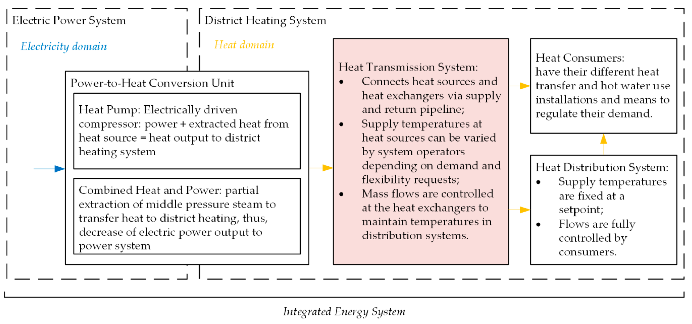
District heating combines heat sources, heat transmission systems and heat distribution systems to which end consumers are connected. DH coupling with an electric power system in an integrated energy system context is shown in
Figure 1.
The transmission system is hydraulically decoupled from each distribution system by a heat exchanger, typically of plate type and counter-current flow arrangement. This decoupling is necessary due to the need to control temperature at sources depending on the expected demand, hydraulic stability, too high temperature of supply water, etc. [
11]. The system with such a decoupling allows greater flexibility in the transmission part, meaning that the electric power consumption can be altered to provide auxiliary services to electric power system, while satisfying DH system operational constraints and the heat demand.
In the distribution system, end consumers regulate mass flows according to their demands. At the time, their supply temperature is kept constant via flow control on the transmission side of the heat substation. The setpoint of the temperature depends on the distribution system design and preferences of the end consumers, as indicated in [
12]. The return temperature level reflects the behaviour of end consumers and the distribution network. In the case of diverse consumption patterns, end equipment and complex distribution networks, this temperature is challenging to predict, unless the distribution part is fully modelled. Numerous works contribute to solving this problem, for instance, in [
13] DH temperature dynamics are addressed and modelling of an existing DH system was performed.
Besides demand changes, deviations in the secondary supply temperature are caused by changes in the primary inlet temperature. These are caused by output temperature changes at the heat source or fluctuations of heat loss in the transmission pipeline due to the mass flow control. All the described processes consequently affect the primary return temperature. Badly optimized supply temperatures will lead to frequent flow control actions in order to maintain the necessary temperature level in the distribution network. Such processes can yield in unpredictable behaviour of the system and cause additional wear on components.
Both supply and return temperatures, as well as the mass flow affect in a non-linear fashion the efficiency of different power-to-heat sources, such as large heat pump (HP) systems or combined heat and power plants (CHP). For electrically driven HPs the ratio of heat output (
) to electric power input (
) is commonly considered, called the total coefficient of performance (
). Given in its simplest form, it is sufficient to express the nonlinearity of the process [
14]:
noting that the temperatures in Equation (1) must be used in the absolute scale (Kelvin).
The power consumption of circulation pumps is significantly lesser than that of heat sources. Their output is controlled against the pressure changes caused by flow control valves at substations. Nevertheless, their power consumption contributes to operational costs and is approximately related to the mass flow rate cubed. Pumping power required for low temperature systems is usually higher, as the supply temperature level at the end consumer has to be maintained.
One of the key problems in DH operation is to find such optimal temperatures and mass flows for the transmission part of the system. This is an operational optimization problem. To formulate the problem mathematically, the following components are the most relevant to model: heat sources, circulation pumps, supply and return pipelines, as well as plate heat exchangers.
2.2. Operational Optimization Problem
Operational optimization in district heating is often regarded as a time-dependent process due to delays (which comprise the flow history) in the network. Moreover, the return temperature is not only affected by delay and demand, but also defined by the past supply temperature. This makes the process of optimization computationally heavy when the mass flow, as well as both supply and return temperatures, are optimized in short time steps (dictated by flexibility provision with power-to-heat solutions) over a certain time horizon.
For the sake of simplicity, in test cases the demand and the price for the electric power are assumed as constants, so the problem transforms into minimization of consumption power in a steady state. This power is divided into power for hot water production () and pumping power (), which together form the objective function. The optimized variables are supply and return temperatures at the source and the transmission mass flow. All three of those variables are essential to include in the optimization as they are essential to quantify available power for system flexibility.
The objective function for the optimization problem is formed as
The power required to produce heat can be obtained from the expression for coefficient of performance (1) as
Power of the circulation pump is the sum of pressure drops over components of the system, including the PHX, supply and return pipes, as well as the condenser of the HP. For the sake of simplicity, the return pipe is assumed to have the same pressure drop as the supply and the condenser is assumed to have the same pressure drop as in the PHX, consisting of port and channel pressure drops. A general expression given as follows:
The pressure drop in pipes is obtained via the Darcy-Weisbach equation, where the friction factor for pipes is determined by an approximation given in [
15]. Equations for the pressure drop in a circuit of PHX are found in [
16]. Thus, Equation (4) can be re-written as follows:
The objective is subjected to constraints, which include maximum and minimum limits for the mass flow and temperatures, as well as heat transfer capability of the heat exchanger and the energy balance between primary and secondary sides:
The constraints indicating minimum and maximum limits of optimized mass flow and temperatures are of linear inequality type. The non-linear equality constraints represent the transferred heat and the heat balance between the sides. The inlet and outlet temperatures of the hot circuit are related to the optimized supply and return temperatures at the heat source via the equation for temperature drop in the pipe, which also includes the mass flow as a part of time delay calculation [
1,
2] as follows:
Thermophysical properties, especially viscosity, vary depending on the temperature of water. These variations cause changes in OHTC , which must be efficiently accounted for. An inaccurate OHTC model can result in non-optimal system operation and frequent control actions, which can further cause temperature and flow oscillations in the system. Thus, detailed modelling and analysis of this coefficient is given in the following section.
3. Modelling and Analysis of Heat Transfer in Plate Heat Exchangers
Modelling and analysis of OHTC is essential to identify models, relevant for the application. The first subsection defines two models, with the difference in whether both cold and hot circuits are treated separately or not, resulting in four approaches to OHTC calculation, two iterative and two with constant thermophysical properties. The second subsection gives analysis on FCC of a circuit, which shows that the thermophysical component can be related directly with temperature. Finally, the third subsection describes the two new models based on results of FCC analysis.
3.1. Modeling of Overall Heat Transfer Coefficient
The calculation of OHTC comprises FCCs from each circuit (
and
) and thermal resistances of plate material and fouling. A complete equation can be written as [
16]:
Forced convection coefficients
and
are related to mass flows and mean temperatures (via thermophysical properties) in cold and hot circuits, respectively. Using a generalized form of the Dittus-Boelter equation for the correlation of Nusselt number, the expression for the convection coefficient [
16] is
Different values for m, n and C are used depending on plate design and prevailing flow conditions. Typically, transition to turbulence in PHX occurs at a low Reynold number. Even at low mass flow rate, the Reynolds number is quite high.
Similar to [
6], after rearranging Equation (9) to get temperature dependent and mass flow dependent parts separated, the expression becomes
where
Following the stated, OHTC Equation (8) can be re-written as
Consequently, if thermophysical properties are assumed to be found for the mean temperature between circuits (“coupling” their mean temperatures into one), Equation (12) turns into
Both Equations (12) and (13) can be used iteratively in the optimization problem. Therefore, (12) and (13) are yielding four approaches for calculation:
- -
Non-iterative coupled based on (13): approach 1.1;
- -
Iterative coupled based on (13): approach 1.2;
- -
Non-iterative decoupled based on (12): approach 2.1;
- -
Iterative decoupled based on (12): approach 2.2.
Approaches 1.1 and 2.1, applied in a district heating context, do not account for temperature changes in the system and define
for the most common temperatures. approaches 1.2 and 2.2 will adjust
iteratively for every temperature change. Lookup tables are used to link temperatures with thermophysical properties, which are further complicating the calculation procedure. It is also worth noting that the resistance component can often be neglected as in [
1].
Direct relation of FCC to a temperature would be more convenient to use. To obtain it, the temperature dependent part (denoted as ) is investigated to use temperature directly instead of thermophysical properties.
3.2. Temperature Dependency of Forced Convection Coefficient
Given the values of the thermophysical properties for water [
17] and applicable values of
n and
m [
18] we can evaluate the function
from temperature. The behavior of
for
m = 0.4 and
n = (0.6, 0.7, 0.8, 0.9) is demonstrated in
Figure 2. Note that thermophysical properties remain nearly constant for the same temperature for any possible pressure in the DH system (the values are taken for
).
As it can be seen from the
Figure 2, the behaviour of function
is very close to linear. Linear regression of
can be applied:
A similar relation for water is described, for instance, in [
19] using the original Dittus–Boelter equation for the case of flow in a circular pipe, where
and
. Linearization coefficients
and
for different
and
combinations are summarized in the
Table 1.
To characterize the goodness of the fit, coefficient of determination
can be found for each approximation (summarized in
Table 2) as
The values confirm that the approximation is very close to the original as they are approaching 1, especially for higher values of .
Thus, it is reasonable to consider that the FCC depends linearly on temperature, while relation with the mass flow is the power of
, which gives us the following expression:
This expression can be used for the FCC estimation using temperature directly, without considering thermophysical properties.
The FCC of a circuit to be found as mean of inlet and outlet coefficients, which in their turn are calculated using inlet and outlet temperatures or directly from the mean temperature of the circuit.
3.3. Resulting Models for Overall Heat Transfer Coefficient
The obtained Equation (16) for the direct relation of FCC with temperature, mapped through a fixed PHX design (represented by
,
and
coefficients) allows transforming temperature decoupled (12) and coupled models (13), respectively:
where
Therefore, two approaches in addition to abovementioned four (1.1, 1.2, 2.1, 2.2) can be outlined:
- -
Coupled linear (18): approach 1.3;
- -
Decoupled linear (17): approach 2.3.
Since the correlations used for the coefficients are approximate in their nature, they perform differently from one system to another. All the described and obtained heat transfer models require experimental verification before applying them in practice. Such verification is provided in the following section.
4. Experimental Verification of Heat Transfer Models
In this section focus is brought to the laboratory PHX as the main component of the setup and the subject of the study. The first subsection describes the setup, measurement sets and datasheet parameters, further continued to the estimation procedure for the correlation and its results in the second subsection. The verification of the models is provided in the third subsection and the simplest means to reduce the correlation error are given in the last subsection.
4.1. Experimental Setup, Parameters and Measured Data
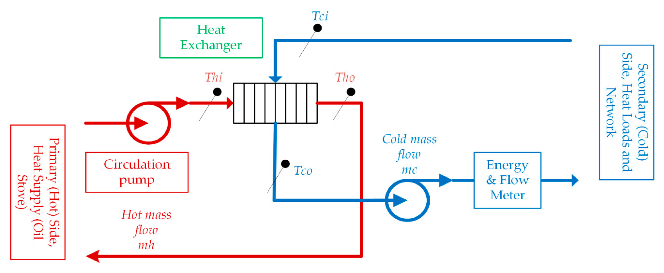
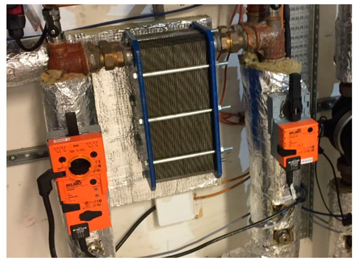
The experimental setup (
Figure 3) consists of a laboratory PHX (
Figure 4) of the counter-flow type, operating in a small heat substation. Hot water in the primary circuit is supplied from the “oil stove” heat source and the heat load (on the secondary side) is represented by two small houses, as well as two small and one large air coolers (dump loads).
PHX parameters, given in the datasheet (manufacturer SPXFlow APV) along with that calculated [
16] and found in the manufacturer’s handbook [
18] are summarized in
Table 3.
Since manufacturers typically do not provide exact values for
,
and
, they have to be estimated within the given range, based on datasheet values and measurements. These include the heat supplied (
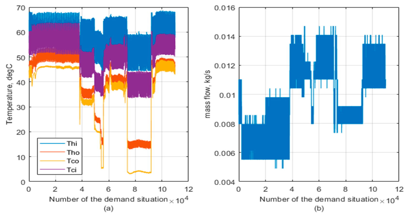
Figure 5) and all four temperatures and mass flow in the cold circuit (
Figure 6), collected by a Kamstrup Multical 602 meter in one-second intervals. Temperatures were measured by thermocouples 745690-J001 (Iron/Constantan).
The whole data consists of five datasets, each obtained over approximately five-hour intervals on a separate day. The datasets were concatenated together. Every time step of the data (1 s) corresponds to a different heat demand situation, and every situation lasts one second and is independent from the other.
The oscillatory behaviour is caused by the heat source operation due to features of the system and crude control. One period corresponds to travel time of water through the primary circuit of the PHX, pipeline and heat source, and can last up to 10 min. The travel time of the secondary circuit (transient) can last from 10 to 30 min, or even more as the circuits of the houses are the longer ones and the circuitry of coolers is the shorter one. The very low secondary inlet (primary outlet) temperature is due to all loads operating during a cold day together with the most powerful cooler.
For estimation purposes, measurements from Datasets 1–3 are used, and for verification purposes—from Datasets 4 and 5.
4.2. Estimation of the Correlation Values
The estimation procedure involves setting up a nonlinear constrained optimization problem (
Figure 7). It was concluded previously that
has a greater effect on the calculation process than the other two parameters [
9]. It also can be seen from Equation (10) that
does not affect the mass flow contribution to heat transfer calculation, while
is a multiplier for both mass flow and thermophysical components. Based on that, we can simplify the procedure by specifying them as constant for all measured sets, i.e.,
and
. Thus, the problem is limited to finding optimal
. A more general and complex approach is used in [
10], where all three values are optimized.
For that purpose, the MATLAB (R2017b, MathWorks, Natick, MA, USA) function
fmincon [
20] was used and the objective is to minimize the difference between the transferred heat calculated by Model (12) and the measured demand.
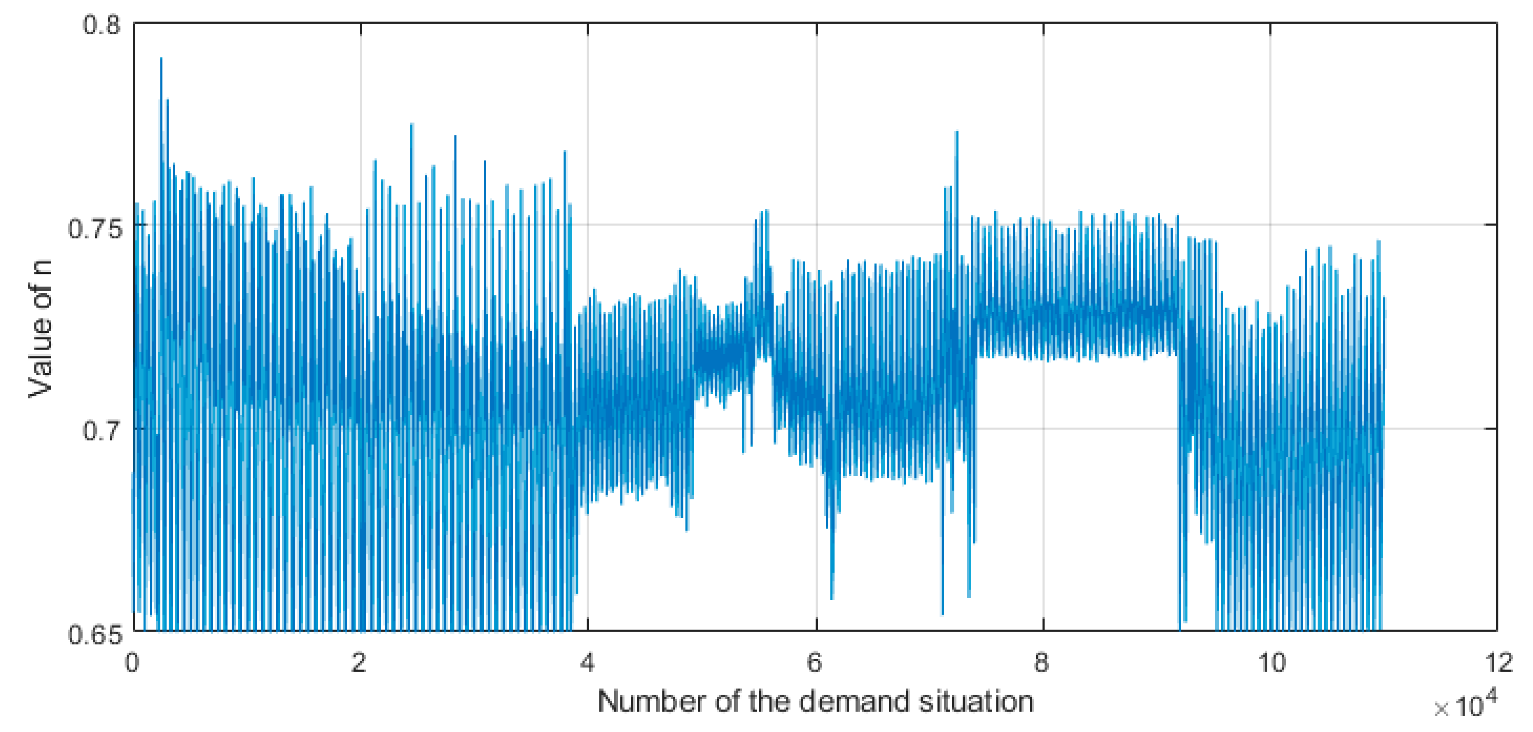
Resulting optimal values of
n for all demand situations are displayed on
Figure 8.
Values of n vary from 0.65 to 0.78 and the weighted mean for estimation datasets is , which corresponds to and after the regression. Those will be used in the following subsection for model verification.
4.3. Verification of Models
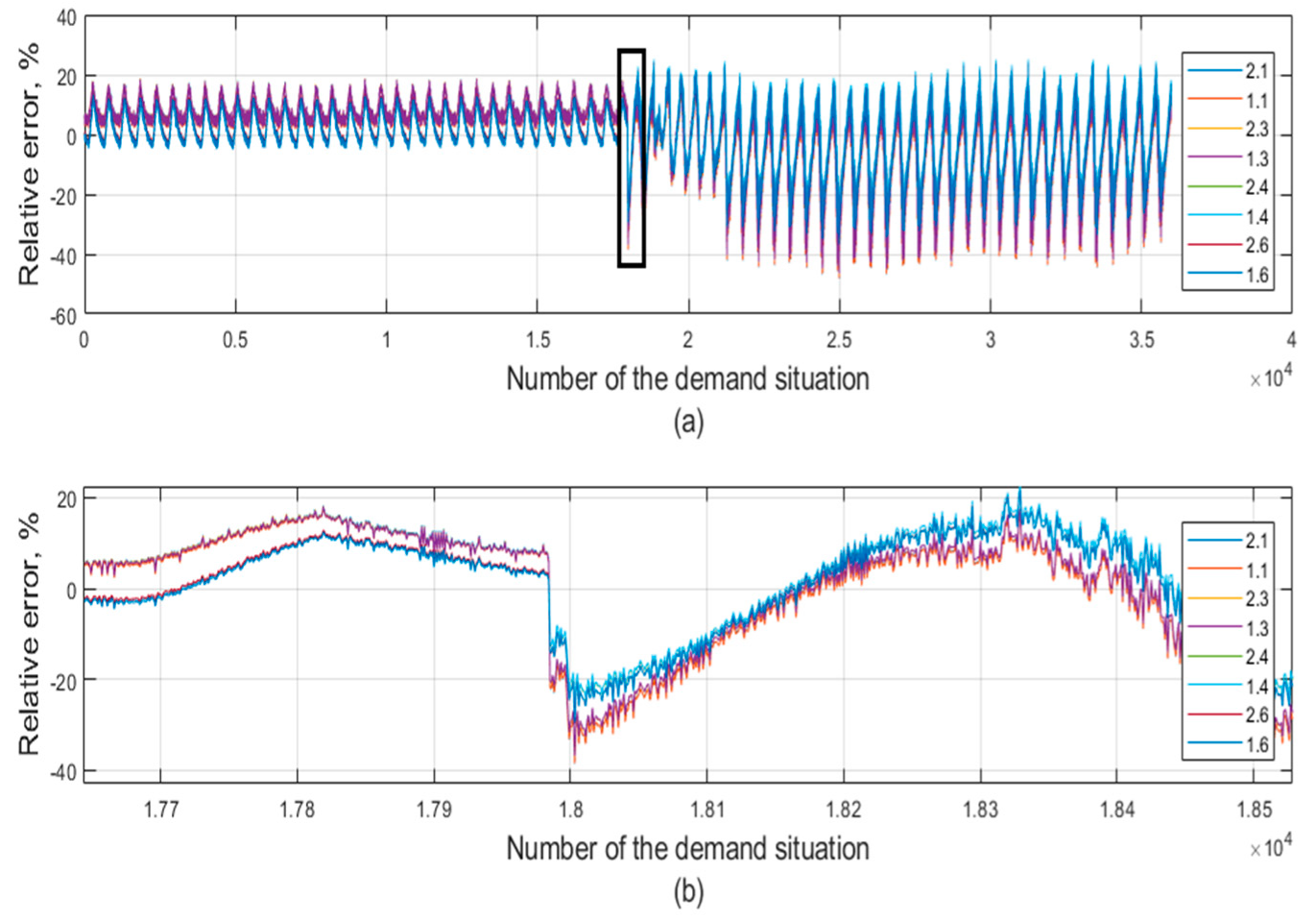
To verify the models, the relative errors calculated by each approach of transferred heat power were compared to the measured one on the secondary side, which is the actual demand. In terms of the relative error,
Performance of each approach in terms of a relative error is shown in
Figure 9, using the demand situations from the verification datasets.
The calculated transferred heat differs from the actual values for the following reasons:
- -
The correlation is an approximation of the complex process of heat transfer;
- -
Measurements themselves have smalls error;
- -
Variable time delay between inlets and outlets in both circuits.
The relative errors between the models almost do not differ:
- -
Thermophysical approach 2.1, a mean temperature for each circuit separately—10.91%;
- -
Thermophysical approach 1.1, one mean temperature for both circuits—10.63%;
- -
Linear regression approach 2.3, a mean temperature for each circuit separately—10.65%;
- -
Linear regression approach 1.3, one mean temperature for both circuits—10.54%.
A negligible difference between all models confirms that linear regression models can be used in practice.
Despite the error being quite high, in general, it can be reduced by collecting more data to cover the whole demand range as well as setting up a “cleaner” experiment overall, e.g., well-tuned controls and properly sized equipment. This is, unfortunately, impossible for the current system due to limited additional demand options, time of the year and continuous operation during certain season.
Further error reduction under existing conditions, without significant complications of the models, can be achieved by changing the value n depending on one of the varying parameters.
4.4. Variable Correlation as a Way to Improve Accuracy
One way to improve accuracy is to further relate n with one or more of varying parameters:
- -
One of mass flows when temperature variations are not significant;
- -
One of circuit temperatures when mass flows variations are not significant;
- -
Mass flow and temperature on one side when parameters on another side vary correspondingly;
- -
Heat load itself, in case most of temperatures and flows are affected by fluctuations.
Since the system behaviour is quite unstable and all parameters are affected by large variations, the value
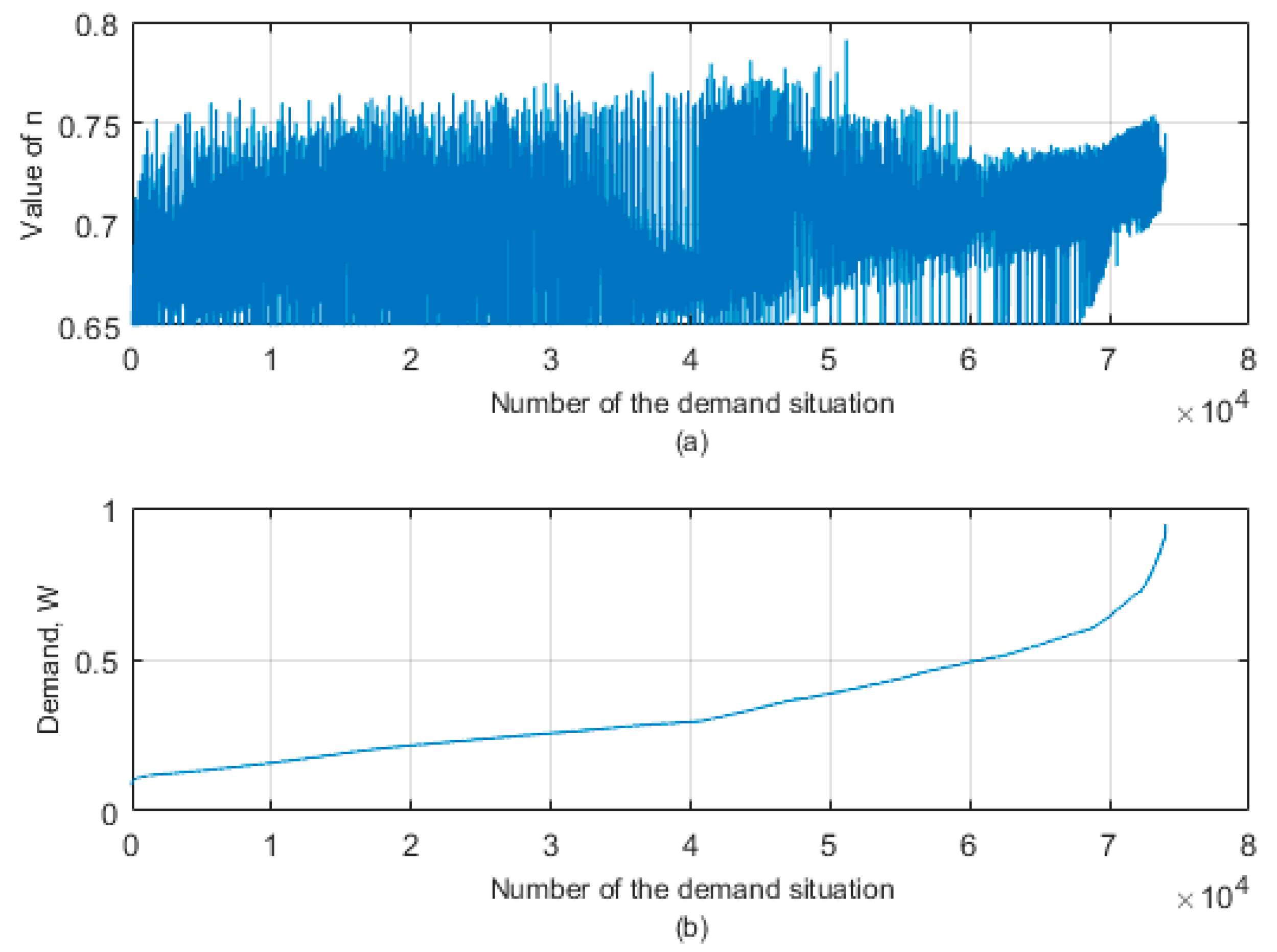
n is related to the heat demand. To relate
n with the transferred heat, let us first re-arrange the obtained values of
n from Datasets 1–3 correspondingly to values of the heat load in an ascending order, as shown in
Figure 10.
Similar to the previous section, linear regression (since simplified solutions are sought) of
n from
Q will result in the expression
Consequently, values
and
can be tied to demand for this particular PHX to enable the use of regression models. Using five points from min (20%) to max (100%) heat load in the expression (20), the respective
and
are summarized in the
Table 4.
This correlation is shown to be nearly linear as we can see from
Figure 11.
A further linear regression will yield
Since Equation (20) is a very “specific” approximation, as well as derived Equation (21), the fit will obviously be poor; however, the relative error for models with those expressions is evaluated and displayed
Figure 12 along with errors from previous models.
The mean relative errors for the variable exponent model with linear regression:
- -
Thermophysical approach 2.4, a mean temperature for each circuit separately—7.40%;
- -
Thermophysical approach 1.4, one mean temperature for both circuits—7.45%;
- -
Linear regression approach 2.6, a mean temperature for each circuit separately—7.67%;
- -
Linear regression approach 1.6, one mean temperature for both circuits—7.61%.
For the variable exponent model with thermophysical properties the error is approximately the same. The iterated versions of approaches 1.4 and 2.4 are denoted as 1.5 and 2.5, respectively.
Mean values of relative errors show that varying the correlation exponent n with a certain parameter (in our case it is heat load) can yield better accuracy. The typical error interval for correlations is ±10%.
The ways of improving heat transfer models remain an open research area and the proposed model is situational. To find the most accurate model, extensive tests are required, covering the entire range for each varying parameter.
5. Results and Discussion on an Operational Optimization Test Case
To demonstrate performance of the obtained models on DH operation, an operational optimization (2) and (6) was performed in a basic heat transmission system under several demand situations. In the first subsection, parameters, configurations and heat demand situations were described. The second subsection presented optimization results, containing values from the reference approach and absolute errors of other approaches as compared to the reference one. The obtained results were followed by a discussion. Finally, the computational performance of each approach is evaluated in the last subsection by optimizing the system with an increasing number of branches.
5.1. System Parameters of the Test Case
The diagram of the test system is shown in
Figure 13. In the first configuration, the PHX is connected to the source via a pipeline and in the second configuration, two identical PHXs are connected via identical separate pipelines and circulation pumps.
Parameters of the test system are listed in the
Table 5. The supply and return pipes are connecting the inlet and outlet of a (each) PHX. A large HP system (power-to-heat source) is extracting heat from the heat source at 6.85 °C (for instance, sea or lake water). The maximum mass flow in all circuits is equally limited (this corresponds to full valve opening). For any PHX in both configurations return cold inlet temperatures and cold mass flows are assumed to get three values as indicated in
Table 5 to comprise a heat demand (thermal load).
Thus, five cases of heat demand are considered for a PHX in Configuration 1:
- -
Common heat demand, when temperature is medium, as well as mass flow;
- -
(2 cases) unbalanced heat demand, when secondary return temperatures and mass flows are both low and high, respectively;
- -
(2 cases) low or high heat demand, which are low mass flow and high temperature or high mass flow and low temperature, respectively.
As for Configuration 2, in order to observe how PHX models perform when several components are present, the following five heat demand cases are considered:
- -
Common heat demand at both PHXs;
- -
(2 cases) unbalanced heat demand with low or high temperatures/flows at one PHX and common at another;
- -
unbalanced heat demand at each PHX, low temperature at one and low mass flow at another;
- -
low heat demand at one PHX and high heat demand at another.
The optimization is performed by each approach, given in previous sections. Since it has been demonstrated that the variable correlation model is the most accurate, it is used as a reference. All the correlation values are taken the same as in previous section and applied for a larger PHX.
Firstly, approach 2.5 is run for the common demand and obtained temperatures are used to find mean temperatures and (defining thermophysical properties) for approaches that do not account for temperature variation. This will yield better performance for them.
5.2. Optimization Results
Optimization procedure is performed using the
fmincon function in MATLAB. The procedure follows the problem, described in
Section 2. We will consider approach 2.5 as our reference since it was shown that thermophysical models with variable correlation are performing better than others. Optimization results for Configurations 1 and 2 are shown in
Table 6.
Other models’ approaches are compared in relation to the reference. Two key indicators are the absolute deviation from the secondary (cold) supply temperature setpoint , assumed ideally coinciding with approach 2.5, and the absolute deviation of total electric power consumed as compared to the one for approach 2.5. Obviously, the deviation of the cold outlet (secondary) temperature will cause a respective deviation of the hot outlet and, moreover, control actions to bring the temperature back to 50 °C (in case of a poorly performing approach) will cause a hot return temperature to further rise and, consequently, affect total electric power consumed.
Procedure of temperature deviation calculation for other approaches related to approach 2.5:
Calculating the OHTC using the complete Equation (12) from provided optimization results, cold side temperatures and mass flow;
Finding the logarithmic mean temperature difference from the given demand, surface area and the OHTC;
Finally, finding such outlet temperatures, which yield equality of the expression for logarithmic mean temperature difference to the found one.
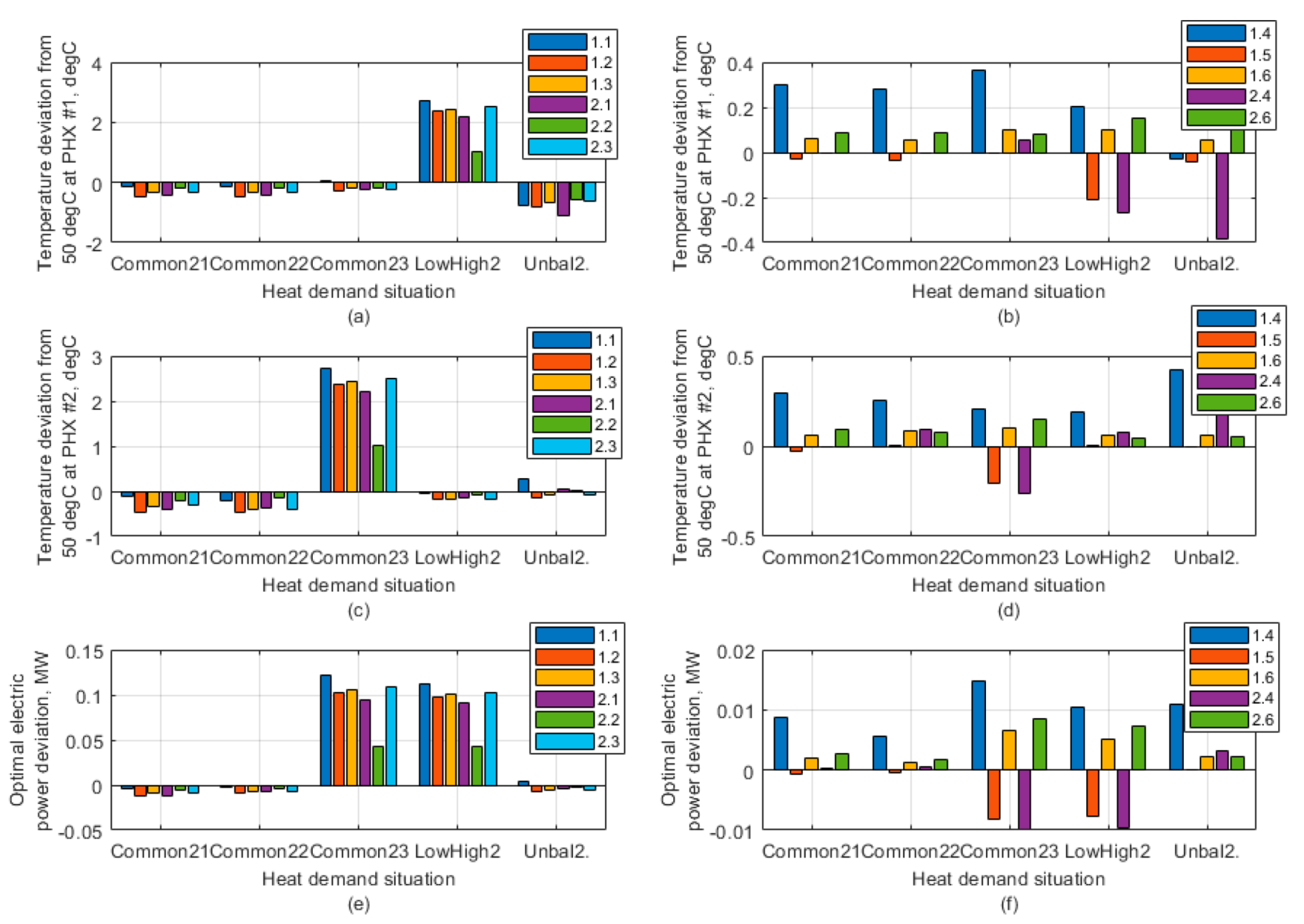
For convenience, two plots are used per one indicator per configuration: for variable correlation approaches and for a fixed correlation. Thus, for Configuration 1 with one PHX and one source there will be four plots total, displayed in
Figure 14.
As we can see from the
Figure 14, the non-variable correlation approaches perform poorly at the second load situation (highest demand), overheating the water by up to 2.5 °C (at least 1 °C for iterative approach 2.2) and drawing up to 100 kW more of electric power. Performance at temperature unbalanced (high cold return temperature/low flow) heat demand is better, but still the temperature deviation is between 0.5 and 1 °C, this time under the setpoint. For common and low heat demands, the temperature deviation is within 0.5 °C, and for mass flow and unbalanced heat demand its deviations are minimal.
All the non-variable correlation approaches perform inconsistently, but approach 2.2 is more robust due to being a non-variable version of the reference approach 2.5.
Variable correlation approaches perform significantly better than their non-variable versions. The maximum temperature deviation is 0.4 °C by Approach 1.4 at Unbal.1M heat demand. For 1.4 and 2.4 the temperature dependence is not included (thermophysical properties are constant, similar to approaches 1.1 and 2.1) and they perform generally worse.
Amongst other approaches, iterative 1.5 performs better, but has a 0.2 °C deviation at high load, whilst approaches 1.6 and 2.6 are more consistent. The highest deviation in electric power consumption among all five is 10 kW by approach 2.4 at high heat demand (corresponds to around a −0.27 °C temperature deviation).
For Configuration 2, there are six plots total, displayed in
Figure 15. This study case is demonstrating how approaches perform in a system. Four of them are temperature deviations at two PHXs and two are the deviations of total electric power consumption.
For non-variable correlation approaches, the temperature and power consumption deviations look similar when both PHX are at common heat demand, also for Configuration 1. Similar to Configuration 1. the trend exhibits PHX (#2) at an unbalanced heat demand with a high temperature difference, which was even amplified by another PHX (#2), unbalanced the other way around and having a low temperature difference but high mass flow on its secondary side. Highest deviations are occurring at high heat demands, at least at one of the PHXs. The magnitude of the deviation is approximately the same as in Configuration 1, with approach 2.2 performing better than other approaches.
For variable correlation approaches, the pattern is similar to Configuration 1, with 1.6 and 2.6 performing the best, 1.4 performing the worst, and 1.5 and 2.4 are being inconsistent.
Generally, the magnitude of errors in Configuration 2 is slightly higher than in Configuration 1, for unbalanced heat demands in particular. Relative errors would be nearly of the same values. Nevertheless, in a real DH system all the pipeline and pumping system, as well as secondary side values and PHXs themselves can differ a lot to one another. Note, those are study aspects (number of which can be dramatically high) for every particular system and will certainly affect approaches performance.
5.3. Computational Performance
Another important criterion (if not the most) is computation time for each approach used. This is becoming crucial when the system is optimized on a short time scale over a greater time horizon (the travel times remain very large). Therefore, the faster we are able to optimize our system, the more flexible it becomes for integration with other energy systems.
We will calculate computation time for each approach versus the system with a number of identical branches with PHX at the end, having the same heat demand for each.
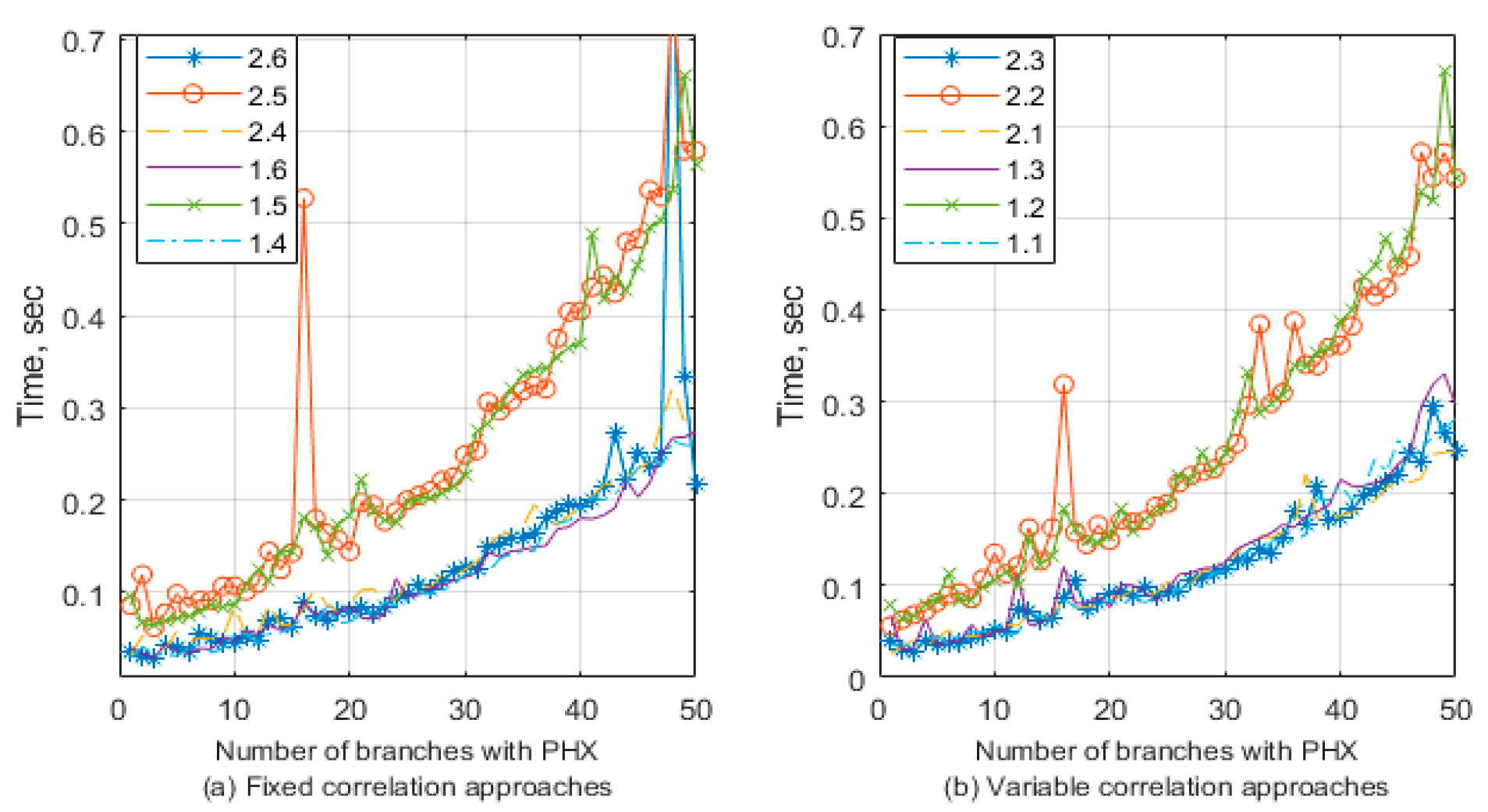
The times can be evaluated in MATLAB using tic-toc commands around the optimization code for each approach. The obtained computation times trend is displayed in
Figure 16: (a) for non-variable correlation approaches and (b) for variable correlation approaches.
As we can see, optimization time grows exponentially with the number of branches in the system. Both variable and fixed correlation approaches take nearly the same time to converge, which favours relating the correlation to a varying parameter, in the case of a heat demand.
Thermophysical iterative approaches (1.2, 2.2, 1.5, 2.5) take twice longer to converge, which means they need at least one more iteration. On the other hand, approaches with linear approximation of temperature dependence take nearly the same time as thermophysical non-iterative approaches, while accuracy is higher and close to the iterative versions as mentioned early in this work.
Additionally, each provided branch has a specific design and setpoints, and the difference in approaches can further raise in favour of the ones with a linear approximation.
6. Conclusions
Flexible operation of DH systems entails significant variations in parameters of DH transmission systems. Defining optimal parameters for the transmission system is the key to maintain sufficient heat quality and minimal operation costs. Even in a relatively small DH system, precise modelling of each individual component can become crucial as the optimization problem includes such models as constraints. Precise modelling of PHX is the most critical for the operation of a transmission system. The better the model fits the reality, the less control effort is required at the heat transfer station afterwards and, therefore, secondary temperature deviations from setpoints will be minimal, especially when demand is unpredictable and flexibility is provided (altering of setpoints). This also means that the primary return temperature and mass flow will be more predictable. Poorly performing models can cause frequent control actions, which result in oscillations in the system, as was seen from the experimental part of this work.
Both mass flows and temperatures affect heat transfer capability of plate heat exchangers. Thus, at various demands plate heat exchangers will produce different return temperatures, which in its turn affects the efficiency of a power-to-heat source (e.g., the heat pump). Especially, this has a greater effect when mass flows and temperatures vary across a wide range, and PHXs, as well as their respective distribution systems, differ significantly in their design (for instance, rating) and demand patterns.
Analysis of heat transfer through DH PHXs has shown that the temperature dependent component of FCC for water has nearly linear behaviour. This persists for the whole range of possible temperatures and covers most of the design correlations, as well as for a large range of pressure since it does not affect thermophysical properties of DH water. This behaviour allows approximating it as a linear function of temperature where and are fixed and defined by the design, which was validated experimentally on a laboratory PHX.
The described linear approximation eliminates the use of lookup tables for thermophysical properties for the calculation of OHTC and, therefore, removes the iterative process from the optimization problem. The approximation use is not limited to district heating only and can be applied whenever the temperature dependent component of FCC for a fluid exhibits linear behaviour.
Correlation estimation procedures, outlined in the experimental part of the work, enables finding the most suitable correlation for a particular PHX from temperature and mass flow measurements. This can be used in practice when inspection of a PHX model is performed. It shows that the correlation accuracy can be further improved by relating its coefficient to one (or several) of the varying parameters.
The two operational optimization study cases show that variable correlation models with linearized temperature dependence perform generally better than the original fixed-temperature thermophysical models, having the same computation time and higher accuracy. The proposed models require at least a two-times lower computation time than variable temperature thermophysical models, while having the same accuracy.
The choice between the models described is made depending on their performance for a specific system and engineering judgement. These, due to some models, are not being consistently good at all heat demands. In real systems, however, with dozens of heat exchangers and multiple power-to-heat sources, the optimization (non-linear control) problem would result in a large number of simulations if all constraints must be satisfied within one optimization interval (time step). Besides, the delays in a DH transmission system can reach a dozen of hours, therefore yielding an enormous number of optimization time steps within the given time horizon. Thus, computational performance is critical.
Detailed modelling and control of power to heat sources, i.e., the coupling units between the sectors, is of high interest, which will be the focus of future work.


