A Fast CFD-Based Methodology for Determining the Cyclic Variability and Its Effects on Performance and Emissions of Spark-Ignition Engines

Abstract

A methodology for determining the cyclic variability in spark-ignition (SI) engines has been developed recently, with the use of an in-house computational fluid dynamics (CFD) code. The simulation of a large number of engine cycles is required for the coefficient of variation (COV) of the indicated mean effective pressure (IMEP) to converge, usually more than 50 cycles. This is valid for any CFD methodology applied for this kind of simulation activity. In order to reduce the total computational time, but without reducing the accuracy of the calculations, the methodology is expanded here by simulating just five representative cycles and calculating their main parameters of concern, such as the IMEP, peak pressure, and NO and CO emissions. A regression analysis then follows for producing fitted correlations for each parameter as a function of the key variable that affects cyclic variability as has been identified by the authors so far, namely, the relative location of the local turbulent eddy with the spark plug. The application of these fitted correlations for a large number of engine cycles then leads to a fast estimation of the key parameters. This methodology is applied here for a methane-fueled SI engine, while future activities will examine cyclic variations in SI engines when fueled with different fuels and their mixtures, such as methane/hydrogen blends, and their associated pollutant emissions.

1. Introduction

Cyclic variations affect the engine performance and emissions, especially in spark-ignition (SI) engines, possibly leading to engine instability regimes in the most extreme cases [1]. In diesel engines this phenomenon is less intensive [2,3], but with similar outputs [4,5]. Its main causes in SI engines are mostly related to the gas properties at the vicinity of the spark plug, such as the mixture velocity and inhomogeneity, the local turbulence level and intensity, as well as the spark plug specifications. Their main result is to affect the flame initiation and propagation, which leads to an overall variation of the combustion process within the engine cylinder [6].

Cyclic variability in SI engines has been extensively examined by several research groups, trying to understand its main causes and ways of resolving these [7]. To this aim, a large diversity of experiments have been conducted focusing on a variety of parameters [8], such as the measurement of the velocity field, flame propagation and specifications [9,10,11,12], and the heat losses to the electrodes of the spark plug [13]. Recently, large focus was also given on the variability of emissions, which requires the use of advanced measuring equipment with a high sampling rate to capture the highly transient effects [14].

At the same time, numerical methodologies for better understanding cyclic variability have been developed. The phenomenological models are mostly used for analyzing the engine performance under such variability [15], while the relevant predictive numerical tools are more scarce [16]. In all cases, this kind of numerical tool does not provide a detailed understanding of the in-cylinder processes. On the other hand, it requires low computational resources, which allows the implementation of even hundreds of multi-cycle simulations within a reasonable time. Therefore, they are particularly useful for multi-parameter numerical studies, focusing on the ones that could affect cyclic variability, relevant to both the engine and its operating conditions [17], and the use of alternative fuels.

The numerical tools that can provide valuable information of the flame propagation at the local level are the ones based on computational fluid dynamics (CFD) [18,19]. Recently, CFD codes based on large-eddy simulation (LES) for investigating cyclic variability in engines have been reported [20], mostly due to the increase of computers power and the advancement of parallel processing. This type of numerical model describes the flow and turbulence phenomena and their interaction with higher detail than the one based on Reynolds-averaged Navier–Stokes (RANS) [21]. However, the former require extremely high computational resources that restrict their multi-cycle simulations up to few tens of consecutive cycles [22]. This is an important constraint for this kind of analysis, especially if the procedure of estimating the coefficient of variance (COV) of the indicated mean effective pressure (IMEP) does not converge.

Even RANS-based CFD models require large computational efforts for this kind of simulation activity [23], but significantly less than the LES-based ones. The multi-cycle simulations can reach up to 100 cycles [24], a number which is adequate for reliable analysis. They are considered a good compromise between the less detailed phenomenological models and the ones based on LES, especially when advanced methodologies are used for dealing with this complex phenomenon. Moreover, they provide valuable information concerning the in-cylinder processes, including the description of the ignition process.

The authors have already developed a 3D CFD RANS-based in-house code for predicting cyclic variability, with an ignition sub-model describing the initial flame kernel growth at the vicinity of the spark plug. This code has been applied in previous studies for the multi-cycle simulation of a methane-fueled SI engine, when considering either only the closed engine cycle [24], or the open cycle as well (i.e., when at least one valve is opened and there is mass transfer between the cylinder content and the inlet/outlet volume) combining the CFD code with a single-zone [25]. In both cases, the closed engine cycle is simulated by the CFD code. These previous works by the authors have shown that even by relying only on the closed engine cycle, reliable results that describe cyclic variability are reached, with the main ones being the COV of IMEP, which has also been compared with the available experimental results. The coupling of single-zone/CFD models increases the runtime, but its overall results are similar to the use of the closed engine cycle only, with negligible discrepancies of performance parameters and small ones of emissions. Therefore, for accelerating the total time needed for this kind of analysis, the current work follows the closed engine cycle approach for the multi-cycle simulations. For comparison purposes in terms of computational time, the first approach requires about 35 days and the latter one 170 days, both for the simulation of 100 cycles in a computer with an Intel-i7 processor.

A methodology is proposed here for further accelerating the computational time needed for this kind of analysis, down to even 2 days for a complete analysis. This is possible, since the key parameter that has been identified to affect the cyclic variability is the relative distance of the spark plug (i.e., the flame initiation location) with the local turbulent eddy calculated at the spark cell. This independent variable introduces a one-way effect on the combustion process of each cycle, while the effect of the previous cycle to the next one is ignored, due to a negligible variation of the flame propagation, as concluded in [25].

Overall, this methodology based on the in-house CFD code allows performance of fast predictions of the main cyclic variability parameters, related to both performance and emissions, over a wide range of operating conditions (e.g., engine load and speed) and fuels (e.g., methane/hydrogen blends). These aspects will be examined in future studies by the authors.

2. Spark-Ignition Engine and Experimental Data

The experimental tests were conducted on a Lombardini LGW 523 MPI, SI engine, modified to burn gaseous fuels [26] and connected to a Tecner E135 Dynamometer. The original engine control unit (ECU) was replaced by a programmable AEM 30-1900 Universal Programmable Engine Management System.

The in-cylinder pressure was measured with a pressure sensor Kistler 6053CC60 installed in the cylinder. Once the engine reached its nominal coolant temperature, and the speed and engine load were stabilized for 90 s, the cylinder pressure was recorded with a National DAQPad 6070E data acquisition card for 300 consecutive cycles.

Moreover, gas analyzers were used to measure the values of both nitrogen oxides (4000 VM NOx chemiluminescence) and carbon monoxide emissions (2100 CO non dispersive infra-red—NDIR). However, only average values were recorded and no cycle-resolved measurements.

The test case examined here concerns a two-cylinder, naturally aspirated test engine with a stoichiometric equivalence ratio of pure methane fuel, operating at a speed of 4500 rpm, and with wide open throttle (WOT). The engine bore/stroke is 72/62 mm, respectively, with a compression ratio of 10.7 and a spark timing at 33° CA BTDC.

The measured data of 300 successive cycles were processed, resulting in a COV of IMEP of 1.83%, which is rather low due to the high engine speed. The COV of peak cylinder pressure (P_max) of this dataset is 7.74%. Further details of this engine and test-rig along with the test facilities are found in [24,27].

3. Numerical Model and Methodology

3.1. Highlights of the CFD Code and Its Main Sub-Models

A research RANS-based CFD code has been already developed for the simulation of the engine closed cycle, using the RNG k-ε turbulence model. A cyclic variability sub-model has been recently added for capturing the relevant effects in spark-ignition engines [24], briefly described in the next sub-section for completeness. The other main sub-models of the CFD code have been validated against experimental data, and they concern the combustion processes with gaseous fuels [28], heat transfer [29] and crevices [30] with dedicated sub-models developed by the authors, and pollutant emissions models [29,30,31,32,33]. The simulations cover the closed engine cycle and start at IVC and finish at EVO. The time step corresponds to 0.5° CA, with the initial values of the gas temperature and pressure equal to 380 K and 1.2 bar respectively. The cylinder liner temperature is equal to 450 K and the piston and cylinder head temperatures equal to 500 K. Further details regarding the initial/boundary conditions and the structured mesh used to describe the cylinder geometry with mesh layers added or removed as the piston travels to the BDC or the TDC, respectively, have been presented in these previous studies.

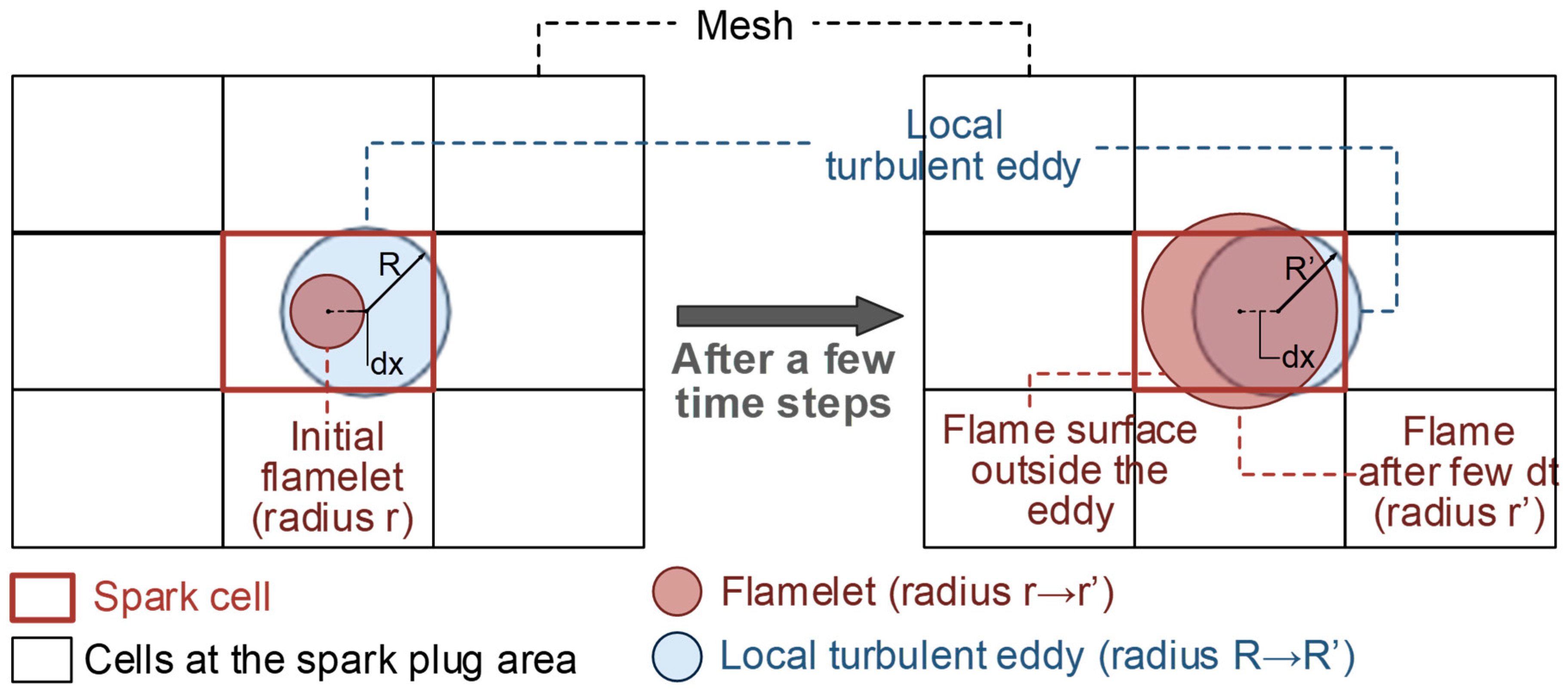
3.2. Brief Description of the Cyclic Variability Sub-Model

The ignition process and the early stages of combustion greatly affect cyclic variation [34]. This process describes the transition from the laminar combustion region to the fully turbulent one, and depends on the relative location of the local turbulent eddy with respect to the initial flame kernel [7].

The ignition sub-model is based on this physical mechanism of flame-turbulence interaction at the spark plug region. The key parameter of this mechanism is the relative position of the initial flamelet at the spark cell with a radius r contained within a turbulent eddy with a radius R, as depicted in Figure 1. They are both assumed to be spheres [35,36] with a distance dx (center to center) that varies over time due to the local fluid flow. The average engine cycle corresponds to the cycle with a distance dx equal to 1/2 of eddy radius, R/2 (equal to ¼ of its diameter) [16]. This cycle gives the mean cylinder pressure with its numerical results being the same once this model is de-activated.

The whole flamelet lies within the local eddy during the very first moments of ignition, propagating with the laminar burning velocity. This flamelet is centered at the computational spark cell [28]. Once a part of the flamelet crosses the boundaries of the eddy outside its periphery (see right part of Figure 1), its burning velocity rapidly starts to accelerate due to the transition to the turbulent region.

The diameter of the local turbulent eddy (equal to 2R) is equal to the turbulent integral length scale, calculated by the gas properties of the spark cell. The radius of the flamelet (equal to r) contained in the spark cell depends on the flamelet radius of the previous time step and the burning velocity [28], and is calculated by Equation (1).

$$r=r_{past}+u_{b,sp}dt,$$

(1)

where r_past is the flame radius at the previous time-step-dt, and u_b,sp is the burning velocity of the gas within the spark cell.

Once the flamelet leaves the spark cell and covers a part of the neighboring grid cells, as shown in the right part of Figure 1, the same procedure is followed. The surface of the flame sphere leaving the eddy is calculated geometrically in all cases, based on the distance of their centers (dx) and their radii.

The surface fraction of the flamelet that lies inside the local eddy propagates with its laminar flame speed, while the flame outside the eddy with its turbulent flame speed. The burning velocity (u_b,sp) is then calculated by Equation (2).

$$u_{b,sp}=\left[u_t{A}_r+u_l\left(1-A_r\right)\right]\frac{{\rho }_u}{{\rho }_b},$$

(2)

where u_t is the turbulent flame speed using the expression proposed by Zimont [37] for its calculation, u_l is the laminar flame speed methane calculated by the expression proposed by Ouimette and Seers [38] for methane, A_r is the surface fraction of the flamelet outside the eddy, and ρ_u, ρ_b are the density of the unburned and burned gas respectively.

During the early stages of combustion, the surface fraction of the flamelet that exits the eddy rapidly increases. The formulation of Equation (2) ensures a smooth transition from the laminar (for A_r equal to zero) to the turbulent (for A_r equal to 1) flame speed.

The next step is to estimate the relative distance of the two spheres, with the aim to correlate this sub-model with the engine cycle variation. For that purpose, a random sample of dimensionless distance (d_n) values in the range of 0–1 was generated. In a previous study, this sample included 100 values. These values are then multiplied by the eddy radius, resulting in a dx distance from 0 (same spheres center) up to R (flame center at the eddy periphery), as shown in Equation (3).

$$dx=R{d}_n,$$

(3)

where d_n is a random number between 0 and 1.

The average cycle corresponds to a d_n value of 0.5 (distance dx = R/2), as already mentioned. The successive d_n values of this sample are provided as input to each closed engine cycle simulation by the CFD code. For higher values, the ignition process is accelerated, resulting in a faster combustion process.

The results are processed for calculating the IMEP of each cycle, as well as the COV of IMEP of all cycles, using Equation (4). The COV of maximum pressure is given by a similar expression shown in Equation (5).

$${COV}_{IMEP}=\frac{\sigma }{\mu }=\frac{\sqrt{\frac{1}{N-1}{\sum }_{i=1}^N{\left({IMEP}_i-{IMEP}_{av}\right)}^2}}{\frac{1}{N}\left({\sum }_{i=1}^N{IMEP}_i\right)},$$

(4)

where σ is the standard deviation of IMEP, μ is the average value of IMEP, N is the number of cycles, IMEP_i is the IMEP value of the i cycle, and IMEP_av is the average IMEP over the N cycles.

$${COV}_{P_{max}}=\frac{\sqrt{\frac{1}{N-1}{\sum }_{i=1}^N{\left(P_{max,i}-P_{max,av}\right)}^2}}{\frac{1}{N}\left({\sum }_{i=1}^N{P}_{max,i}\right)},$$

(5)

where P_max,i is the maximum pressure of the i cycle, and P_max,av is the average maximum pressure over the N cycles.

In [24] it has been shown that 73 cycles need to be simulated for this methodology to converge, based on the convergence criterion applied.

3.3. The Fast Methodology for Estimating the Key Parameters of Cyclic Variability in SI Engines

It becomes clear that there is a one-way dependence of the multi-cycle simulations from the d_n value. Therefore, the methodology is based on simulating a small (representative) sample of engine cycles. A d_n step of 0.25 was selected, resulting in the simulation of just five cycles in total, using the RANS-based CFD code.

The main results of these engine cycles were then collected, and the main parameters of interest processed, such as the IMEP and the peak pressure. For these parameters along with the emissions, a regression analysis was followed to produce fitted correlations of high accuracy as a function of the above relative distance. These correlations were then used for calculating the main parameters and emissions over several (hundred) cycles in a spreadsheet.

The results of concern are the IMEP, peak pressure, angle of peak pressure, NO and CO emissions of these five cycles. For the test engine, the results related to performance values are shown in Figure 2 (IMEP, peak pressure and its angle) and the ones related to emissions in Figure 3 (NO and CO-dry), together with the fitted correlations. For all parameters and emissions, a 4th order polynomial is needed to reach a R² equal to 1, except from the peak pressure that a 2nd order is adequate.

The peak pressure is varied by about ±5 to 6 bar around its average value directly affecting its angle of occurrence, which is highly advanced for the fast burning cycles. However, this has a small effect on the engine IMEP with an absolute variation of ±0.2 bar around its average value, which is less than 2.5%.

The result that is affected to the largest extent by this relative distance is the NO emissions [25], which increase by more than three times over the whole range of d_n values. The outcome is a large scattering of NO under a normal engine operation even with a low COV of IMEP. On the other hand, CO emissions show a minor variation, having higher values in the slow burning cycles with a low d_n value, since their production in the combustion chamber is not favored at elevated temperatures, as is the case with NO.

The main aspect to be initially examined in the Results section is the accuracy of this methodology compared to the complete multi-cycle simulations of the CFD code, presented in [24]. The next step is the extension of the number of cycles to even 1000, which is not possible to be simulated by a CFD code. Finally, the distribution of the main parameters and emissions is examined when a very large number of cycles with a random sample of d_n values is used.

4. Results and Discussion

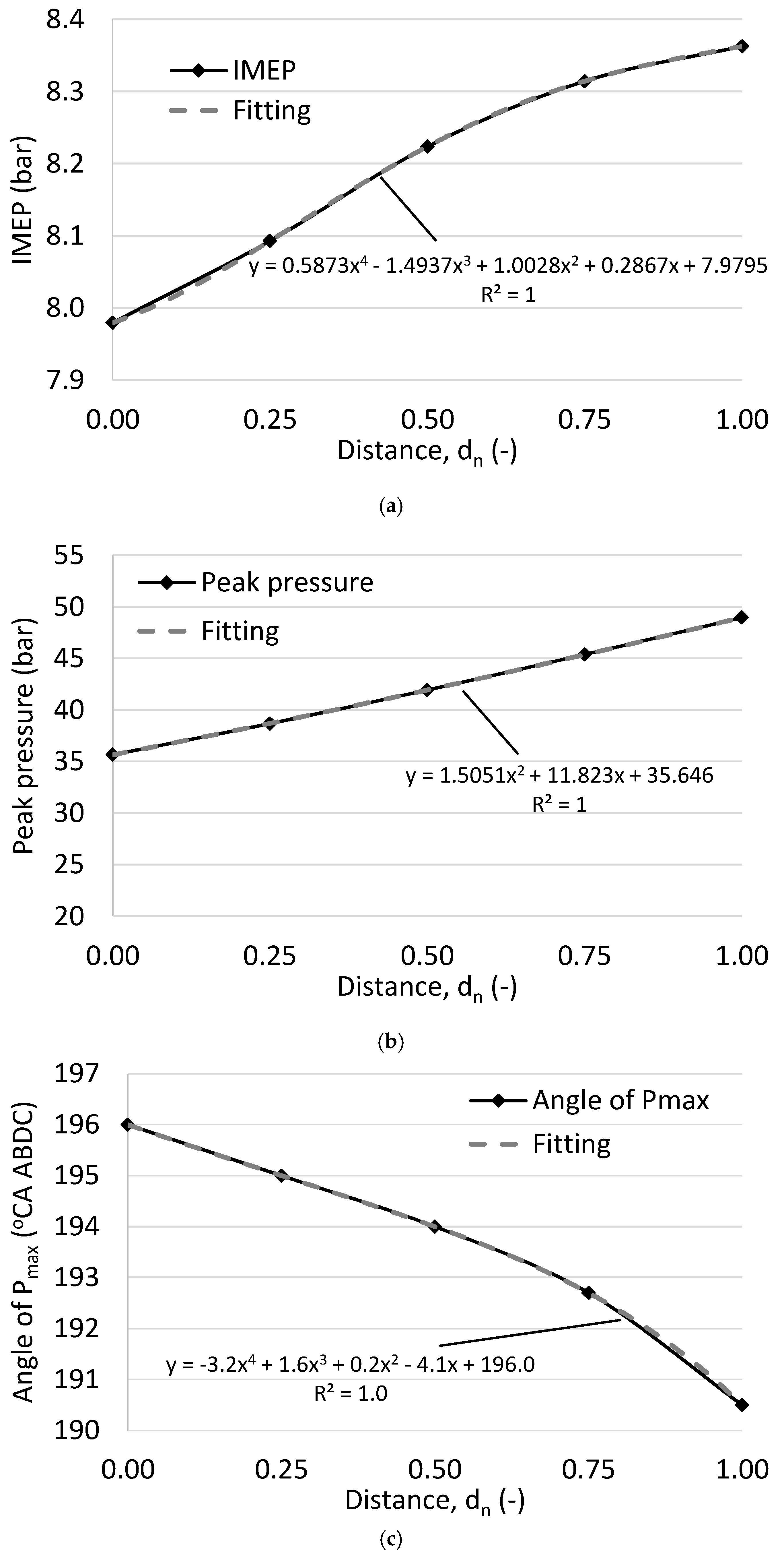
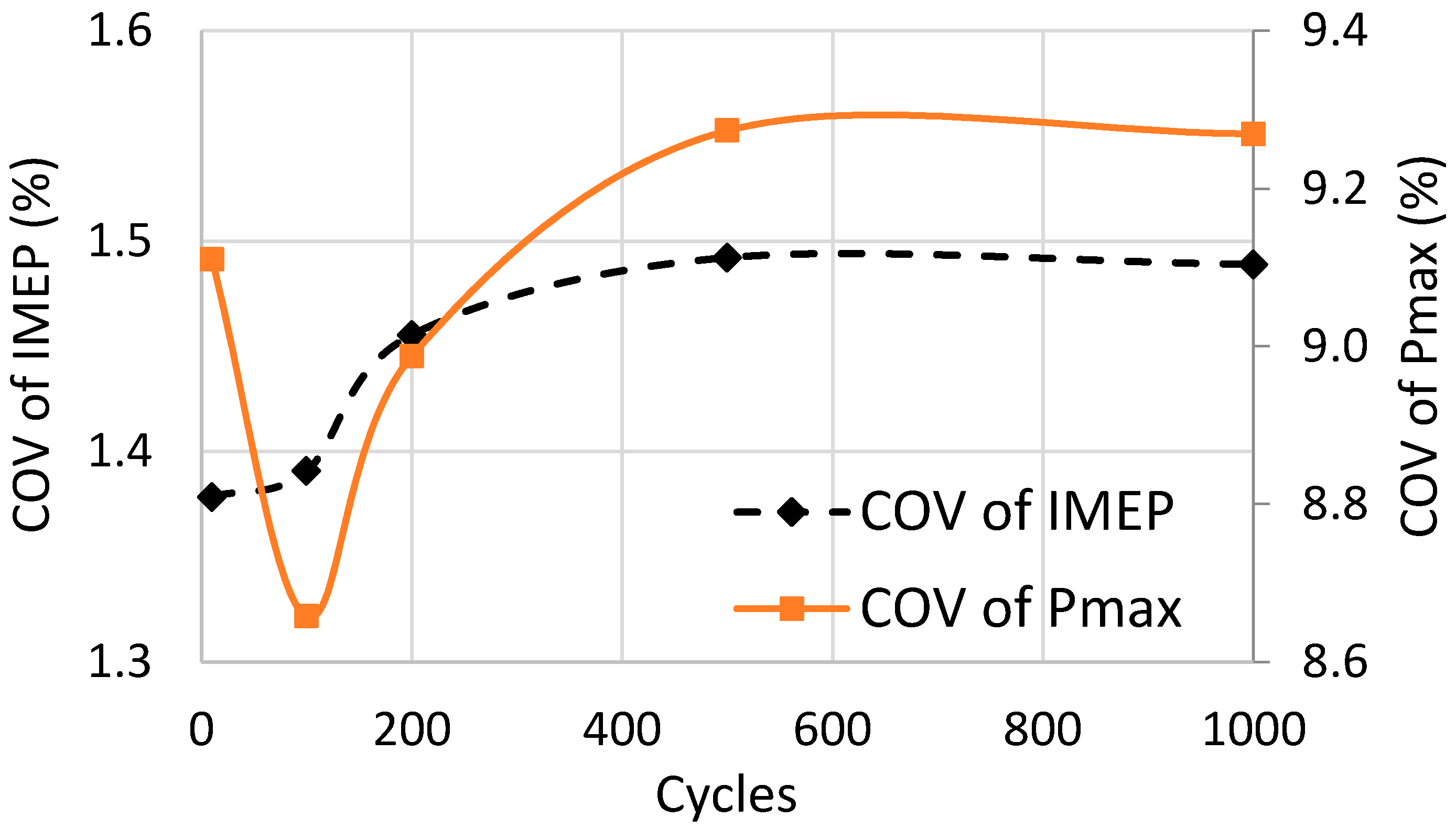
4.1. Cyclic Variability of Engine Performance

The effect of cyclic variability was initially examined on the performance of the tested SI engine fueled with pure methane, running at an engine speed of 4500 rpm. For that purpose, the COV of IMEP and peak pressure are given in Figure 4, as a function of the different number of cycles from 10 up to 1000 cycles. These two parameters are crucial for determining the stability of the engine.

Based on the results and the convergence criterion presented in [24], 73 cycles were adequate with a resulting COV of IMEP of 1.38%. From the test data, a COV value of 1.83% is obtained (25% difference). It is clearly shown in Figure 4 that a larger number of cycles are needed, of over 500, in order to secure the global convergence. This is possible only with the fast methodology presented in this work, resulting in a COV of IMEP equal to 1.49%, reducing the relative variation compared to the experimental data to 19%.

The COV of peak pressure shows a similar behavior, again needing over 500 cycles for final convergence to a value of 9.27%. For 73 cycles it is equal to 8.74%, as presented in [25], while the COV of peak pressure based on the test results is 7.74%. This deviation of 20% could be caused by additional mechanisms that contribute to the cyclic variability and not captured by the methodology presented, even if the open engine cycle is also included in the simulations [25]. There are continuous efforts by the authors to include additional mechanisms and increase the reliability of the numerical results, always within reasonable computational effort.

The distribution of the peak pressure is presented next, in order to identify whether the relevant numerical results approach the normal distribution. This type of distribution for the peak pressure is usually observed according to test data [25]. The frequency of the peak pressure, as calculated by the presented methodology for a different number of cycles, as well as the experimental one, is shown in Figure 5.

The distribution in the case of over 100 cycles approaches the normal one, being similar to the experimental case, while for only 10 cycles large discrepancies are observed due to the very small sample. The frequency for the cycles with peak pressure close to the average one is about 18%, while for the experimental one is 23%.

The monitoring of the peak pressure is important, since it is a useful indicator to determine the state of the cyclic variability, except from the IMEP. The angle at which this peak is observed also determines whether the cycle is a slow or fast burning cycle, as previously presented in Figure 2c. The peak pressure and its angle of occurrence are presented in Figure 6 as a function of the IMEP for the case where 1000 cycles are included in the analysis, also highlighting the average IMEP of about 8.2 bar. For fewer cycles, the results are similar.

When a higher peak pressure is observed the IMEP is increased, as also highlighted previously. The previous rapidly decreases the angle of the peak pressure by almost 5° CA, shortening the combustion duration by a greater extent. This is depicted in Figure 7, where the durations for 0–5%, 5–95%, and 0–95% of mass fraction burned (MFB) are shown as a function of the IMEP, for the case with 1000 cycles with a random d_n value.

The advancement of the peak pressure for the fast burning cycles (up to 5° CA) is less than half compared to the acceleration of the whole combustion process, which is up to 14 CA deg. Large differences are observed especially for the 0–5% duration, which points towards the flame initiation process, which is greatly affected by the location of the local turbulent eddies. This duration is reduced by up to 8.5° CA, while another reduction of up to 5.5° CA is introduced during the main combustion process, which corresponds to the 5–95% of MFB duration.

The above results clearly show that the effect of the flame initiation process, in which the flame is within the spark plug vicinity, contributes to the whole combustion process more than the following processes.

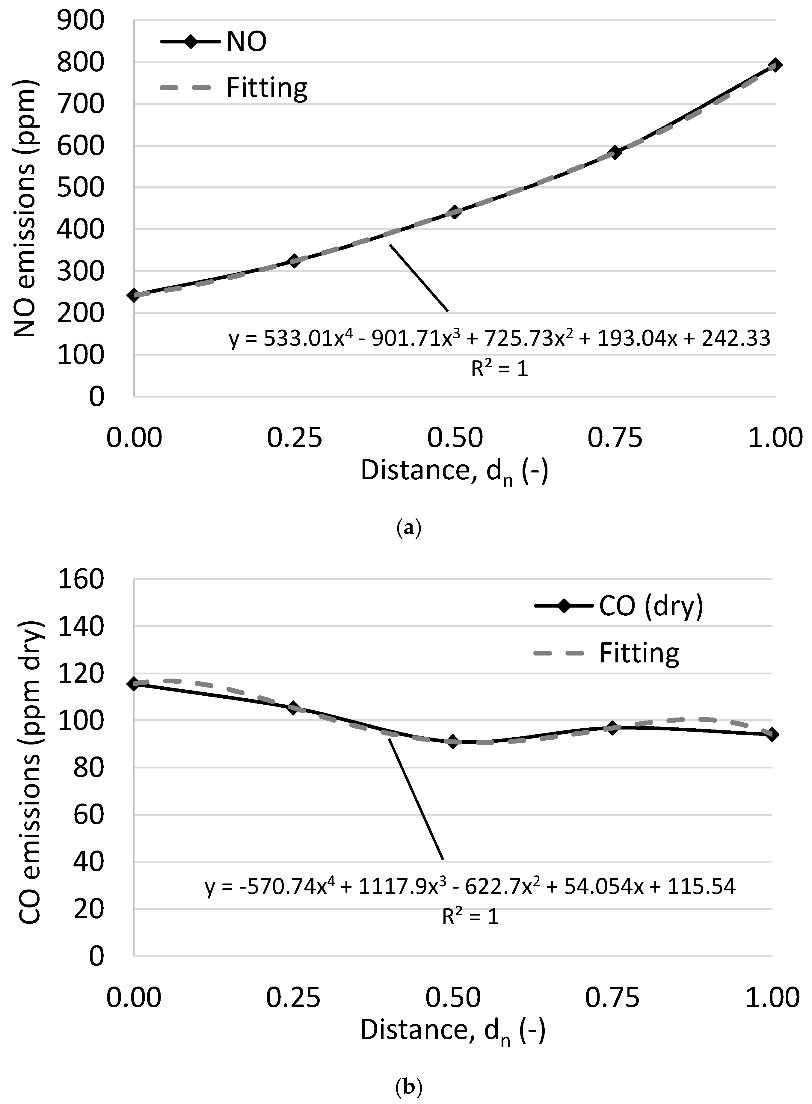
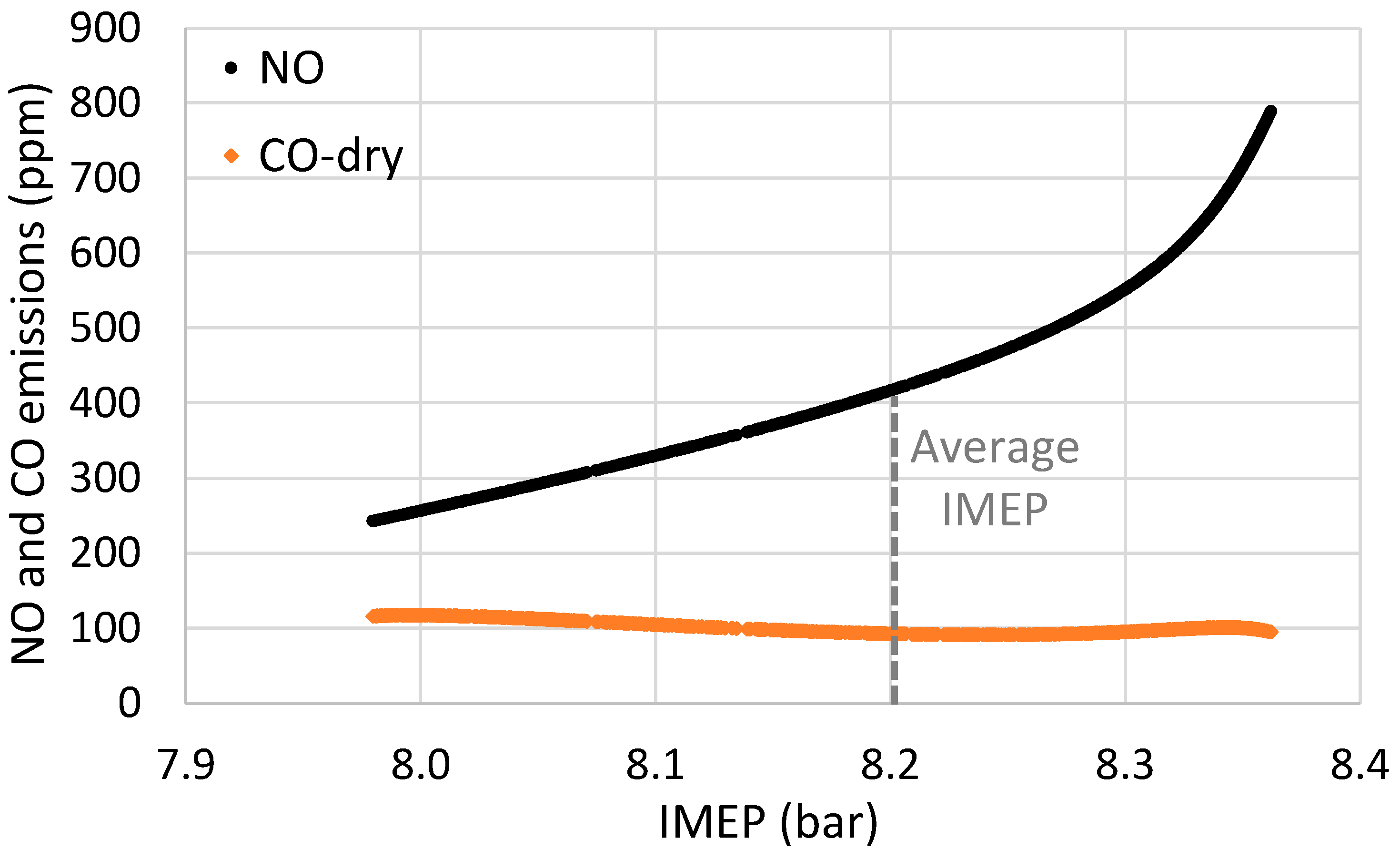
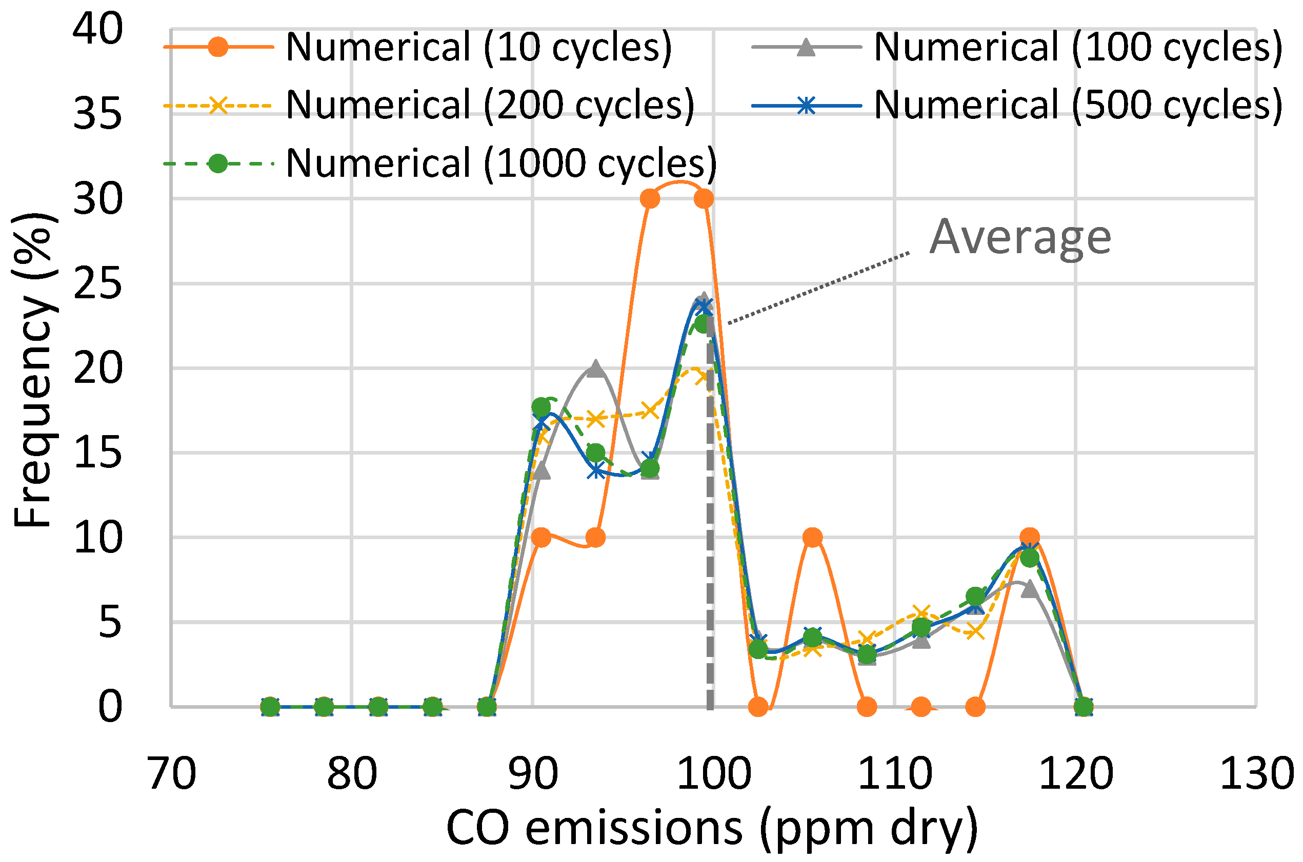
4.2. Cyclic Variability of Emissions

The cyclic variability effects on emissions have started recently to attract much attention, with the aim to determine their variation [14,39]. The work here focuses on NO and CO emissions, which are the main pollutants for SI engines. These are presented next for determining their cyclic variability in the test engine.

4.2.1. NO Emissions

In a previous work by the authors, when the open engine cycle was also included in the 73 multi-cycle simulations [25], a large cyclic variability of NO emissions has been observed. The distribution of these emissions was wide with many cycles producing NO 50% less than the average one, but with a significant share of cycles having NO emissions much higher. Here the number of cycles was expanded up to 1000 cycles, with the resulting distribution of the NO emissions shown in Figure 8.

The skewness of NO emissions is clear with many cycles producing twice as high NO than the average value. This is a direct outcome of the combustion speed, with the fast cycles having much higher gas temperatures especially at the core of the combustion chamber, which greatly favors the NO production. This is presented in Figure 9, where the NO and CO emissions are given as a function of the IMEP for the case of 1000 cycles.

It should be noted here that the average NO emissions over the 1000 cycles is 464 ppm, while the cycle with the average IMEP gives about 410 ppm of NO.

4.2.2. CO Emissions

A similar analysis is provided for the CO emissions as well. Their distribution over a different number of cycles is shown in Figure 10.

The narrow distribution observed is around the mean value of 100 ppm, almost the same as the CO emitted by the cycle with the average IMEP (equal to 91 ppm), as shown in Figure 9. Therefore, it seems that the engine cyclic variability has a small effect on CO emissions, shifting the focus on NO emissions as presented previously.

5. Conclusions

A fast methodology for determining the cyclic variability in SI engines was developed, extending the previous efforts by the authors in this field. The main feature of this methodology is that it requires very few complete CFD simulations of the closed engine cycle, even just five representative cycle simulations. This reduces the necessary computational time to less than 2 days, allowing the investigation of various set-ups and operating conditions. By processing the results of these five cycles, the analysis of many cycles can be then achieved with quick calculations, focusing on both performance and emissions parameters, such as the COV of IMEP and peak pressure, and the variability of NO and CO emissions.

The results showed that a very large number of cycles are needed for final convergence, which is not possible to be reached with multi-cycle CFD simulations. On the other hand, the methodology presented is appropriate for such high numbers of cycles, which is its main advantage. The converged COV of IMEP is equal to 1.49%, closer to the experimental one compared to previous relevant works by the authors.

Then, the distribution of the IMEP was examined, when a different number of cycles were examined. The analysis showed that even with 100 cycles it is possible to reach a qualitatively correct distribution, similar to the normal distribution and the one obtained based on the test data. The results relevant to the engine performance were also related to the timing of the peak pressure and how this defines the fast combustion cycle, in which the flame initiation process is greatly accelerated, corresponding to the 0–5% of MFB duration.

On the emissions part, the cyclic variability introduces a very large scattering of NO emissions, with the fast combustion cycles producing twice as high NO than the average cycle. Their distribution is skewed, with the NO for the majority of the cycles being at the lower end. On the other hand, CO emissions are slightly influenced by the cyclic variability with a small deviation around their average value of about 100 ppm dry.

The future work of the authors is related to extending the presented methodology, as well as applying it for analyzing the cyclic variability in SI engines when fueled with different fuels and blends, and at different operating conditions. This kind of analysis with the use of a CFD tool is possible only with the approach presented in this work, since it concerns multi-cycle simulations for several different cases, requiring tremendous computational resources that are not yet reachable within reasonable times.

References

1. Truffin, K.; Angelberger, C.; Richard, S.; Pera, C. Using large-eddy simulation and multivariate analysis to understand the sources of combustion cyclic variability in a spark-ignition engine. Combust. Flame 2015, 162, 4371–4390. [Google Scholar] [CrossRef] [Green Version]
2. Labeckas, G.; Slavinskas, S.; Kanapkienė, I. The individual effects of cetane number, oxygen content or fuel properties on the ignition delay, combustion characteristics, and cyclic variation of a turbocharged CRDI diesel engine—Part 1. Energy Convers. Manag. 2017, 148, 1003–1027. [Google Scholar] [CrossRef]
3. Rakopoulos, C.D.; Rakopoulos, D.C.; Kosmadakis, G.M.; Papagiannakis, R.G. Experimental comparative assessment of butanol or ethanol diesel-fuel extenders impact on combustion features, cyclic irregularity, and regulated emissions balance in heavy-duty diesel engine. Energy 2019, 174, 1145–1157. [Google Scholar] [CrossRef]
4. Rakopoulos, D.C.; Rakopoulos, C.D.; Kyritsis, D.C. Butanol or DEE blends with either straight vegetable oil or biodiesel excluding fossil fuel: Comparative effects on diesel engine combustion attributes, cyclic variability and regulated emissions trade-off. Energy 2016, 115, 314–325. [Google Scholar] [CrossRef]
5. Rakopoulos, D.C.; Rakopoulos, C.D.; Giakoumis, E.G.; Komninos, N.P.; Kosmadakis, G.M.; Papagiannakis, R.G. Comparative evaluation of ethanol, n-butanol, and diethyl ether effects as biofuel supplements on combustion characteristics, cyclic variations, and emissions balance in light-duty diesel engine. J. Energy Eng. 2016, 143, 4016044. [Google Scholar] [CrossRef]
6. Ozdor, N.; Dulger, M.; Sher, E. Cyclic Variability in Spark Ignition Engines a Literature Survey; SAE Technical Paper 940987; SAE International: Warrendale, PA, USA; Troy, MI, USA, 1994. [Google Scholar]
7. Hill, P.G. Cyclic variations and turbulence structure in spark-ignition engines. Combust. Flame 1988, 72, 73–89. [Google Scholar] [CrossRef]
8. Karvountzis-Kontakiotis, A.; Ntziachristos, L.; Samaras, Z.; Dimaratos, A.; Peckham, M. Experimental investigation of cyclic variability on combustion and emissions of a high-speed SI engine. In Proceedings of the SAE 2015-01-0742; SAE Technical Paper; SAE International: Warrendale, PA, USA, 2015. [Google Scholar]
9. Aleiferis, P.G.; Hardalupas, Y.; Taylor, A.; Ishii, K.; Urata, Y. Flame chemiluminescence studies of cyclic combustion variations and air-to-fuel ratio of the reacting mixture in a lean-burn stratified-charge spark-ignition engine. Combust. Flame 2004, 136, 72–90. [Google Scholar] [CrossRef]
10. Brown, A.G.; Stone, C.R.; Beckwith, P. Cycle-By-Cycle Variations in Spark Ignition Engine Combustion-Part I: Flame Speed and Combustion Measurements and a Simplified Turbulent Combustion Model; SAE Technical Paper 960612; SAE International: Warrendale, PA, USA; Troy, MI, USA, 1996. [Google Scholar]
11. Fontana, G.; Galloni, E. Experimental analysis of a spark-ignition engine using exhaust gas recycle at WOT operation. Appl. Energy 2010, 87, 2187–2193. [Google Scholar] [CrossRef]
12. Huang, B.; Hu, E.; Huang, Z.; Zheng, J.; Liu, B.; Jiang, D. Cycle-by-cycle variations in a spark ignition engine fueled with natural gas–hydrogen blends combined with EGR. Int. J. Hydrogen Energy 2009, 34, 8405–8414. [Google Scholar] [CrossRef]
13. Beretta, G.P.; Rashidi, M.; Keck, J.C. Turbulent flame propagation and combustion in spark ignition engines. Combust. Flame 1983, 52, 217–245. [Google Scholar] [CrossRef] [Green Version]
14. Karvountzis-Kontakiotis, A.; Dimaratos, A.; Ntziachristos, L.; Samaras, Z. Exploring the stochastic and deterministic aspects of cyclic emission variability on a high speed spark-ignition engine. Energy 2017, 118, 68–76. [Google Scholar] [CrossRef]
15. Stone, C.R.; Brown, A.G.; Beckwith, P. Cycle-By-Cycle Variations in Spark Ignition Engine Combustion—Part II: Modelling of Flame Kernel Displacements as a Cause of Cycle-By-Cycle Variations; SAE Technical Paper 960613; SAE International: Warrendale, PA, USA; Troy, MI, USA, 1996. [Google Scholar]
16. Tinaut, F.V.; Giménez, B.; Horrillo, A.J.; Cabaco, G. Use of Multizone Combustion Models to Analyze and Predict the Effect of Cyclic Variations on SI Engines; SAE Technical Paper 2000-01-0961; SAE International: Warrendale, PA, USA; Troy, MI, USA, 2000. [Google Scholar]
17. Rakopoulos, C.D.; Rakopoulos, D.C.; Mavropoulos, G.C.; Kosmadakis, G.M. Investigating the EGR rate and temperature impact on diesel engine combustion and emissions under various injection timings and loads by comprehensive two-zone modeling. Energy 2018, 157, 990–1014. [Google Scholar] [CrossRef]
18. Forte, C.; Corti, E.; Bianchi, G.M.; Falfari, S.; Fantoni, S. A RANS CFD 3D Methodology for the Evaluation of the Effects of Cycle by Cycle Variation on Knock Tendency of a High Performance Spark Ignition Engine; SAE Technical Paper 2014-01-1223; SAE International: Warrendale, PA, USA; Troy, MI, USA, 2014. [Google Scholar]
19. Vermorel, O.; Richard, S.; Colin, O.; Angelberger, C.; Benkenida, A.; Veynante, D. Towards the understanding of cyclic variability in a spark ignited engine using multi-cycle LES. Combust. Flame 2009, 156, 1525–1541. [Google Scholar] [CrossRef]
20. Granet, V.; Vermorel, O.; Lacour, C.; Enaux, B.; Dugué, V.; Poinsot, T. Large-Eddy Simulation and experimental study of cycle-to-cycle variations of stable and unstable operating points in a spark ignition engine. Combust. Flame 2012, 159, 1562–1575. [Google Scholar] [CrossRef] [Green Version]
21. Van Dam, N.; Rutland, C. Understanding in-cylinder flow variability using large-eddy simulations. J. Eng. Gas Turbines Power 2016, 138, 102809. [Google Scholar] [CrossRef]
22. D’Adamo, A.; Breda, S.; Berni, F.; Fontanesi, S. Understanding the origin of cycle-to-cycle variation using large-eddy simulation: Similarities and differences between a homogeneous low-revving speed research engine and a production DI turbocharged engine. SAE Int. J. Engines 2019, 12, 79–100. [Google Scholar] [CrossRef]
23. Scarcelli, R.; Sevik, J.; Wallner, T.; Richards, K.; Pomraning, E.; Senecal, P.K. Capturing Cyclic Variability in Exhaust Gas Recirculation Dilute Spark-Ignition Combustion Using Multicycle RANS. J. Eng. Gas Turbines Power 2016, 138, 112803. [Google Scholar] [CrossRef]
24. Kosmadakis, G.M.; Rakopoulos, D.C.; Arroyo, J.; Moreno, F.; Muñoz, M.; Rakopoulos, C.D. CFD-based method with an improved ignition model for estimating cyclic variability in a spark-ignition engine fueled with methane. Energy Convers. Manag. 2018, 174, 769–778. [Google Scholar] [CrossRef]
25. Kosmadakis, G.M.; Rakopoulos, D.C.; Rakopoulos, C.D. Performance and emissions of a methane-fueled spark-ignition engine under consideration of its cyclic variability by using a computational fluid dynamics code. Fuel 2019, 258, 116154. [Google Scholar] [CrossRef]
26. Arroyo, J.; Moreno, F.; Muñoz, M.; Monné, C.; Bernal, N. Combustion behavior of a spark ignition engine fueled with synthetic gases derived from biogas. Fuel 2014, 117, 50–58. [Google Scholar] [CrossRef]
27. Moreno, F.; Arroyo, J.; Muñoz, M.; Monne, C. Combustion analysis of a spark ignition engine fueled with gaseous blends containing hydrogen. Int. J. Hydrogen Energy 2012, 37, 13564–13573. [Google Scholar] [CrossRef]
28. Rakopoulos, C.D.; Kosmadakis, G.M.; Pariotis, E.G. Evaluation of a combustion model for the simulation of hydrogen spark-ignition engines using a CFD code. Int. J. Hydrogen Energy 2010, 35, 12545–12560. [Google Scholar] [CrossRef]
29. Rakopoulos, C.D.; Kosmadakis, G.M.; Pariotis, E.G. Critical evaluation of current heat transfer models used in CFD in-cylinder engine simulations and establishment of a comprehensive wall-function formulation. Appl. Energy 2010, 87, 1612–1630. [Google Scholar] [CrossRef]
30. Rakopoulos, C.D.; Kosmadakis, G.M.; Dimaratos, A.M.; Pariotis, E.G. Investigating the effect of crevice flow on internal combustion engines using a new simple crevice model implemented in a CFD code. Appl. Energy 2011, 88, 111–126. [Google Scholar] [CrossRef]
31. Kosmadakis, G.M.; Rakopoulos, C.D. Computational fluid dynamics study of alternative nitric-oxide emission mechanisms in a spark-ignition engine fueled with hydrogen and operating in a wide range of exhaust gas recirculation rates for load control. J. Energy Eng. 2015, 141, C4014008. [Google Scholar] [CrossRef]
32. Kosmadakis, G.M.; Rakopoulos, D.C.; Rakopoulos, C.D. Investigation of nitric oxide emission mechanisms in a SI engine fueled with methane/hydrogen blends using a research CFD code. Int. J. Hydrogen Energy 2015, 40, 15088–15104. [Google Scholar] [CrossRef]
33. Kosmadakis, G.M.; Rakopoulos, D.C.; Rakopoulos, C.D. Methane/hydrogen fueling a spark-ignition engine for studying NO, CO and HC emissions with a research CFD code. Fuel 2016, 185, 903–915. [Google Scholar] [CrossRef]
34. Hinze, P.C. Cycle-To-Cycle Combustion Variations in a Spark-Ignition Engine Operating at Idle; Massachusetts Institute of Technology: Cambridge, MA, USA, 1997. [Google Scholar]
35. Tabaczynski, R.J.; Trinker, F.H.; Shannon, B.A.S. Further refinement and validation of a turbulent flame propagation model for spark-ignition engines. Combust. Flame 1980, 39, 111–121. [Google Scholar] [CrossRef]
36. Hires, S.D.; Tabaczynski, R.J.; Novak, J.M. The Prediction of Ignition Delay and Combustion Intervals for a Homogeneous Charge, Spark Ignition Engine; SAE Technical Paper 780232; SAE International: Warrendale, PA, USA; Troy, MI, USA, 1978. [Google Scholar]
37. Zimont, V.L. Gas premixed combustion at high turbulence. Turbulent flame closure combustion model. Exp. Therm. Fluid Sci. 2000, 21, 179–186. [Google Scholar] [CrossRef] [Green Version]
38. Ouimette, P.; Seers, P. Numerical comparison of premixed laminar flame velocity of methane and wood syngas. Fuel 2009, 88, 528–533. [Google Scholar] [CrossRef]
39. Kyrtatos, P.; Zivolic, A.; Brückner, C.; Boulouchos, K. Cycle-to-cycle variations of NO emissions in diesel engines under long ignition delay conditions. Combust. Flame 2017, 178, 82–96. [Google Scholar] [CrossRef]
Figure 1. Relative location of initial flamelet and local turbulent eddy at the spark plug region. Left part: at spark ignition; Right part: after a few time steps.
Energies 12 04131 g001
Figure 2. (a) Indicated mean effective pressure (IMEP), (b) peak pressure, and (c) angle of peak pressure for the five representative cycles with a different dn value. Their fitted correlations are also shown, together with the R2.
Energies 12 04131 g002
Figure 3. (a) NO, and (b) CO (dry) emissions for the five representative cycles with a different dn value. Their fitted correlations are also shown, together with the R2.
Energies 12 04131 g003
Figure 4. Coefficient of variation (COV) of IMEP and peak pressure for a different number of cycles.
Energies 12 04131 g004
Figure 5. Frequency of peak pressure for a different number of cycles and comparison with the measured one.
Energies 12 04131 g005
Figure 6. Peak pressure and its angle as a function of the IMEP for the case of 1000 cycles.
Energies 12 04131 g006
Figure 7. Combustion duration as a function of the IMEP for the case of 1000 cycles.
Energies 12 04131 g007
Figure 8. Frequency of NO emissions for a different number of cycles.
Energies 12 04131 g008
Figure 9. NO and CO-dry emissions as a function of the IMEP for the case of 1000 cycles.
Energies 12 04131 g009
Figure 10. Frequency of CO emissions (dry) for a different number of cycles.
Energies 12 04131 g010