Computer Model for Financial, Environmental and Risk Analysis of a Wind–Diesel Hybrid System with Compressed Air Energy Storage

Abstract

Remote and isolated communities in Canada experience gaps in access to stable energy sources and must rely on diesel generators for heat and electricity. However, the cost and environmental impact resulting from the use of fossil fuels, especially in local energy production, heating, industrial processes and transportation are compelling reasons to support the development and deployment of renewable energy hybrid systems. This paper presents a computer model for economic analysis and risk assessment of a wind–diesel hybrid system with compressed air energy storage. The proposed model is developed from the point of view of the project investor and it includes technical, financial, risk and environmental analysis. Robustness is evaluated through sensitivity analysis. The model has been validated by comparing the results of a wind–diesel case study against those obtained using HOMER (National Renewable Energy Laboratory, Golden, CO, United States) and RETScreen (Natural Resources Canada, Government of Canada, Canada) software. The impact on economic performance of adding energy storage system in a wind–diesel hybrid system has been discussed. The obtained results demonstrate the feasibility of such hybrid system as a suitable power generator in terms of high net present value and internal rate of return, low cost of energy, as well as low risk assessment. In addition, the environmental impact is positive since less fuel is used.

1. Introduction

Canada has one of the widest territories in the world, it has a dense population in the south but very scarce in the north. Northern regions count with many remote areas and isolated villages unconnected to the national grid. As a result, diesel gensets are used as main source of electricity. However, the main drawbacks of this solution include: the cost to generate a kilowatt-hour of electricity versus the associated fuel procurement cost [1,2,3], the environmental impact of using fossil fuels [4] versus the system efficiency [5]. One way to tackle these issues is the use of renewable energy systems. The provinces of Quebec and Newfoundland and Labrador are filled with abundant wind resources making well suited for the deployment of hybrid systems. Wind–diesel hybrid system with compressed air energy storage (WDCAS) appears as a cost-effective alternative to supply electricity and to ensure diesel generator operational efficiency. The combination of these sources with an energy storage system (ESS) helps to balance variations in power supply and demand.

A wind–diesel hybrid system is a stand-alone power system with wind and diesel generators. These systems are recommended for medium scale applications when the use of diesel generators is unavoidable. ESS integration facilitates a hybrid stand-alone system to optimize energy usage while maintaining efficient demand response. Compressed air energy storage (CAES) appears as an economically mature technology. Cost, simplicity, lifespan, fuel consumption and greenhouse gas (GHG) emissions are all influential factors that determine the competitiveness of this technology for wind–diesel hybridization. Moreover, CAES represents a promising solution to store electricity derived from kinetic energy of air at a particular time for further utilization.

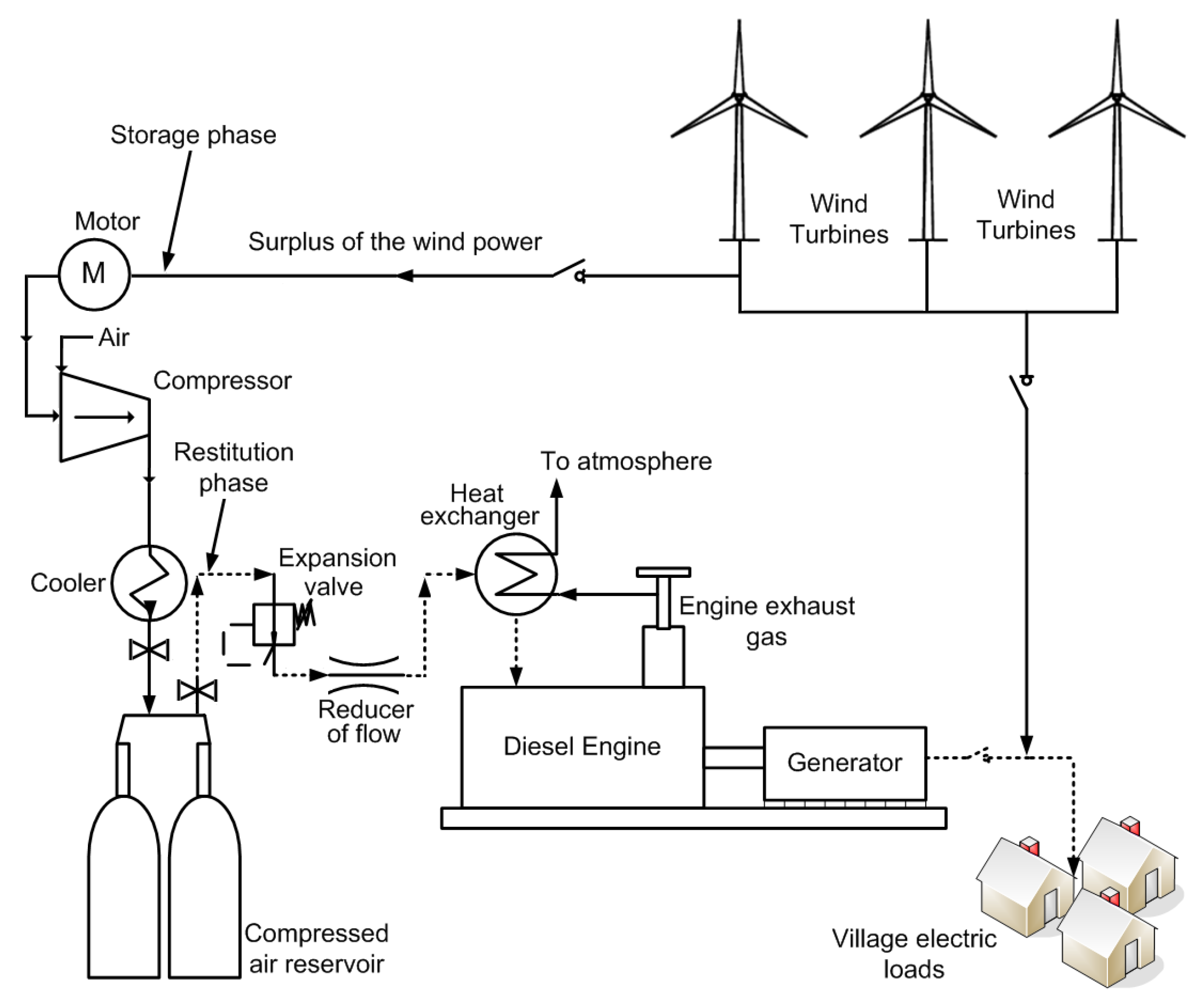
WDCAS operates according to compression-decompression cycles. The overall performance is subject to load power requirements, energy sources availability and energy storage level. The principle consists of two main phases. During high wind speed conditions, the excess of air is compressed and stored in a reservoir, when the energy is needed, the stored compressed air is released to drive a turbo-generator for electricity production. During low wind speed conditions, wind energy is also privileged by the system, thereby power is supplied by the WT and the diesel generator is used to make up for the difference. Figure 1 presents the system overview, which includes the primary energy source (diesel), the renewable energy source (wind) and the compression and storage system (compressor and reservoir). Ancillary systems should be included to ensure safe operation and energy efficiency management in the hybrid system.

Zhang et al. [6] proposed an adiabatic CAES system with variable configuration to cope with the large amplitude wind power fluctuations. Results suggest that after system integration the rate of wind power connected to the grid is increased from 26.29% to 70.62%. In addition, an economic analysis was done determining a net present value of 26.5 million USD and a payback period of about eight years. A similar study is presented in Reference [7]. A techno-economic analysis was carried out to evaluate the potential profitability of developing a wind system with CAES for power generation.

A thermal-economic model was developed by Marano et al. [8] using dynamic programming to optimize the operating strategy of a wind–solar hybrid system with CAES. Their study was focused on environmental and economic analysis with the purpose of minimize operational costs. The obtained results show an average reduction of 80% with respect to the conventional scenario wherein the user load is supplied by the power grid, while ${\mathrm{CO}}_2$ emissions can be reduced by a factor of 74%.

Salvini [9] conducted a techno-economic analysis of a CAES system integrated into a small-size gas steam combined cycle plant. The economic analysis focused on plant performance and investments costs. To determine the best CAES power configuration, the storage pressure and the pressure at the beginning of the charging phase were varied to further obtain storage efficiency values in a range of 58 to 65%. The results have shown that the initial investment is rather high and depends on the cost of the storage unit, which in turns is influenced by the storage capacity. However, the authors concluded that the proposed system may be considered of interest since it is a mature technology with a high durability.

Adefarati et al. [10] studies the optimal configuration of key performance indicators such as fuel, operation and energy costs of a hybrid system composed of WT, PV, diesel generator and battery storage system. Simulation results from four system configurations are obtained by using HOMER software. Results suggest that incorporate WT and PV reduced the operating cost of the hybrid system. Kaabeche et al. [11] analyze three configurations in a stand-alone hybrid system. A comparison between PV/wind/battery, PV/wind/diesel/battery and diesel generator only scenarios are presented. A techno-economic analysis was made by using the total energy deficit, the total net present cost and the energy cost as main criteria for optimization. Results suggest that PV/wind/diesel/battery exhibit the most economically suitable configuration to fulfill the load demands and minimize the cost of energy production. In Reference [12], authors developed a model to study financial and environmental benefits in the use of a Vanadium Redox Battery as ESS in a wind farm.

Another study determining the profitability of a PV wind–diesel hybrid system is presented in Reference [13]. The authors assess the impact on the optimal system design as a function of the daily electrical energy consumption and the meteorological data of the site. The final goal was to maximize the long-term savings in a ten years period for each proposed solution with respect to a diesel–only configuration.

In this work, a computer model has been developed. The model is composed of two parts: one part consisting of system design and technical analysis [14], the other one consisting of financial, environmental and risk analysis. The scope of this paper is focused on the second part of the WDCAS software. The remaining sections are organized as follows: in Section 2, the mathematical formulation of the proposed model is briefly presented. In Section 3, an economic analysis and risk assessment of a WDCAS implementation is described. Simulation results obtained from WDCAS (Wind Energy Research Laboratory, Rimouski, QC, Canada), HOMER and RETScreen software are compared and discussed in Section 4. In addition, the feasibility study applied to the particular case of a mining camp in a remote area in northeastern province in Canada is covered and discussed. Concluding remarks are presented in Section 5.

2. WDCAS Software: System Modeling and Operating Strategy

2.1. Model-Based System Design

In this section, the mathematical models of the major components associated with the WDCAS are briefly introduced. Equation (1) represents the energy balance between the energy produced and the energy consumed. For a given time step $t_{step}$, power generation is estimated in function of the load, the wind resource, the diesel genset and the energy stored level.

$$P_{Load}=P_{WT}+P_{DG}-P_{CAES}$$

(1)

2.1.1. Load

A load profile must be provided by the user. In particular, the dataset contains the amount of energy typically taken during each hour by a consumer or class of consumers over a defined period. According to the load profile, the WDCAS software estimates the total power required by each subsystem.

2.1.2. Wind Turbine

WT performance is estimated by using the wind power curve combined with the WT type used and the wind characteristics of the site under study. Wind power curve represents the relationship between the power available from the wind $P_{WT}$ and the wind speed $v_w$. The WDCAS software uses the wind power curve and the wind speed distribution to estimate the total energy produced by a WT over a specific period of time. The Weibull probability distribution is used to model the wind speed, as defined in Equation (2).

$$f\left(v_w\right)=\left(\frac{k}{c}\right){\left(\frac{v_w}{c}\right)}^{k-1}exp\left[-{\left(\frac{v_w}{c}\right)}^k\right]$$

(2)

where k and c refer to the shape and scale factors, respectively. These parameters should be provided by the user following a wind speed measurement campaign or from wind atlases or meteorological databases in case this information is unknown. By default, for a given $v_w$, k is assumed to be two (Rayleigh distribution) and c is calculated.

System configuration, operation strategies and economic parameters can be adapted through the wind penetration level [15]. WPPR in Equation (3) is defined as the ratio of the installed wind power capacity to the system peak load demand.

$$WPPR=\frac{P_{W{T}_{max}}}{P_{Loa{d}_{max}}}$$

(3)

According to the selected value of WPPR, the WDCAS software determines the number of WT needed by using Equation (4).

$$N{B}_{WT}=\frac{P_{Loa{d}_{max}}WPPR}{P_{WT}}$$

(4)

2.1.3. Diesel Generator

A computational model has been built based on the models described in Reference [16]. The WDCAS software allows using one or more diesel generator units to operate in dual-mode: “normal mode” without compressed air for overcharging and/or “supercharged mode” with compressed air. In normal operating mode, fuel consumption is calculated based on diesel generator power $P_{DG}$. This can be done using Equation (5) below.

$${\dot{m}}_{f_{DG}}=A{P}_{DG}-B$$

(5)

where A and B are specific parameters for each diesel generator.

In supercharged operating mode, the stored compressed air is used to keep optimal efficiency by controlling the stoichiometric air/fuel ratio $\lambda$. Equation (6) shows the mathematical expression of air and fuel supplied for combustion.

$$\lambda =\frac{{\dot{m}}_{i{n}_{DG}}}{{\dot{m}}_{f_{DG}}}$$

(6)

where ${\dot{m}}_{i{n}_{DG}}$ is the air mass flow entering the engine.

Previous studies have shown that maximum efficiency of diesel generators of about ${\eta }_{DG}\approx 56\%$ can be achieved for an air/fuel ratio of $\lambda \approx 53$ [16]. Therefore, the WDCAS software considers this optimal ratio for all overcharged operation regimes. Equation (7) shows the fuel and compressed air flow rates required to supercharge the diesel generator, where ${\eta }_{DG}\approx 56\%$.

$$P_{DG}=PCI{\eta }_{DG}{\dot{m}}_{f_{DG}}=PCI{\eta }_{DG}\frac{{\dot{m}}_{i{n}_{DG}}}{\lambda }$$

(7)

2.1.4. Compressed Air Storage

The compressor type exert a significant influence over the load and the size of the storage tank. The WDCAS software does not count with predefined compressors parameters; the user should configure them according to technical, economic and logistic considerations. For a multi-stage compressor, the compressor power $P_C$ is defined by Equation (8).

$$P_C=\frac{n_C{N}_C}{n_C-1}{\dot{m}}_{C}R{T}_{st}\left[{\left(\frac{p_{o{u}_C}}{p_a}\right)}^{\frac{n_C-1}{n_C{N}_C}}-1\right]{\displaystyle \frac{1}{{\eta }_{p_C}}}$$

(8)

where $n_C$ is the polytropic index, $N_C$ is the number of compressor stages, ${\dot{m}}_C$ is the compressed air mass flow rate through the compressor, R is the perfect gas constant and $T_{st}$ is the storage temperature. In addition, $p_{o{u}_C}$, $p_a$ and ${\eta }_{p_C}$ are the outlet pressure, the inlet atmospheric pressure and the polytropic efficiency of the compressor, respectively.

$P_C$ also can be expressed as the wind power surplus $P_{W{T}_{ex}}$ adjusted with respect to the electric efficiency ${\eta }_{e_{WT}}$ of the WT and the transmission efficiency ${\eta }_{tr}$ between the electric motor and the compressor, as presented in Equation (9).

$$P_C=P_{W{T}_{ex}}{\eta }_{e_{WT}}{\eta }_{tr}=\left(P_{WT}-P_{Load}\right){\eta }_{e_{WT}}{\eta }_{tr}$$

(9)

2.1.5. Storage Tank

A tank is used under pressure air storage. For a given $t_{step}$, it supplies the compressed air flow required to supercharge the diesel generator and to balance the load power demand. In Equation (10), the capacity of a storage unit ${\dot{m}}_u$ is defined under the assumption that maximum efficiency of diesel generators of about ${\eta }_{DG}\cong 56\%$ can be achieved for an air/fuel ratio of $\lambda \cong 53$.

$${\dot{m}}_u=\frac{\lambda P_{Loa{d}_{ave}}}{{\eta }_{DG}PCI}$$

(10)

The total volume of the storage system is calculated in Equation (11).

$$V_{st}=\frac{N_{uni{t}_{max}}{\dot{m}}_{u}R{T}_{st}}{p_{st}}$$

(11)

where the maximum number of storage units required is a constant defined as:

$$N_{uni{t}_{max}}=N{D}_{auto}\times 24·3600\frac{t_{step}}{1\mathrm{hour}}$$

(12)

where $N{D}_{auto}$ is the number of days in which the system will be able to operate without wind power generation and in supercharged mode. This parameter should be provided by the user.

2.2. System Operating Strategy

WDCAS performance is evaluated according to the operating strategy chosen by the user (e.g., wind penetration level, compressed air stored in the reservoir, etc.). For each case, the developed computer model enables to determine system operational parameters over a complete year. Different operating scenarios of the hybrid system can be considered. Although the main objective of this study is to simulate the operation of a wind–diesel system with CAES, it is possible to simulate a system with diesel generators or a wind–diesel without ESS. Each scenario is designed under the constraint that diesel generators should not work below 30% of their nominal power rate. Moreover, when the system operates with a scenario using a WT, the use of wind power to generate electricity is privileged by the system. Thus, if wind power production is the lowest for a given load profile, diesel generators are used to fill the gap.

Different system configurations were simulated using WDCAS software, then a parametric analysis has been conducted to analyze the impact of key parameters on the energy efficiency of the hybrid system. Finally, a decision matrix has been built to find the optimal strategy. The decision matrix is formed for a specific set of criteria with an assigned weight, as follows:

• Fuel economy (0.275): As the primary purpose of the project is to reduce fuel consumption and operation costs, this is the most important criterion advantage if the proposed system allows reducing fuel consumption compared to the original system.
• System complexity and impact of diesel generator failure (0.225): Due to the site remoteness, the system should not be too complex to ensure a quick and easy maintenance. The loss of a generator should have the least impact on the security of supply.
• Energy management system (0.1): This criterion considers the concept of security of supply as larger the power that can be divided between the systems, lesser the impact of losing one of them. However, care must be taken that the system is not too complex.
• Wind turbine failure (0.075): Despite it can affect the efficiency of the system; the loss of a wind turbine does not affect the safety of the installation.
• Storage capacity and power dissipation (0.05): Their influence will be more a logistical constraint.

The choice of the optimal configuration is made based on the overall score resulting from the system classification. The best solution is not necessarily the one with best fuel economy but the one with the best compromise between the whole selected criteria.

3. WDCAS Software: Financial, Risk and Environmental Analysis

In this section, the set of indicators used for financial analysis, risk and environmental assessment of the studied WDCAS are presented. The developed software estimates the overall costs and revenues. It includes the feasibility study, the design and development of the hybrid system, as well as the annual fees for operation and maintenance (O&M).

3.1. Financial Analysis

This module provides financial information about the system. It helps the user to see annual revenues in a chart or graphically. It also provides financial indicators for decision making.

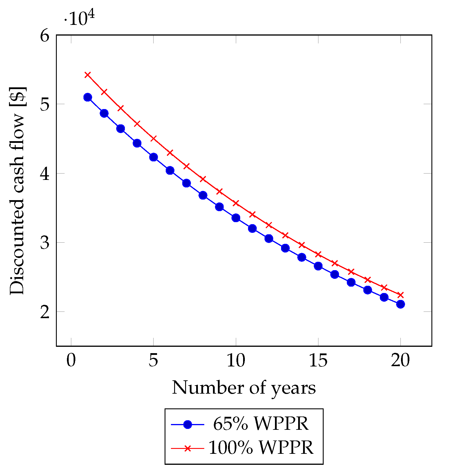
3.1.1. Net Present Value (NPV)

NPV is defined as the value updated to the present moment by means of an adequate rate of interest, of all future charges and payments that a project is expected to generate. Time value of money dictates that cash flows in different time periods cannot be accurately compared; they must be adjusted to reflect their equivalent value at the same period of time. Having in mind these concepts, the NPV can be calculated using Equation (13):

$$NPV=\sum _{t=1}^n\frac{A_t}{{(1+r)}^t}-I$$

(13)

where $A_t$ corresponds to the cash flow during year t, r is the discount rate, I is the initial capital or the initial investment and n is the project life in years.

3.1.2. Internal Rate of Return (IRR)

IRR is defined as the discount rate that equates the present value of the investment in a project with the present value of the cash inflows from the project. The IRR is calculated based on Equation (13) except that rather than solving for NPV, the NPV is set to zero, as result:

$$NP{V}_{IRR}=0$$

(14)

$$\sum _{t=1}^n\frac{A_t}{{(1+IRR)}^t}-I=0$$

(15)

According to Equation (15), IRR is calculated by iteration until the desired precision is reached. Since n is the length of the analysis period, a rate of return for an investment greater than the time value of money is profitable.

3.1.3. Payback Period (PP)

It refers to the time period required for the cumulative cash flow expected from an investment in a project to recover the original cost of the investment. Unlike NPV and IRR, the PP does not take into account the time value of money.

$$PP=\frac{I}{A_{c_t}}$$

(16)

In the discounted payback period (DPP), the interest rate is introduced to determine the present value of future costs and benefits. The interest rate is considered in the same way as described in Equation (13).

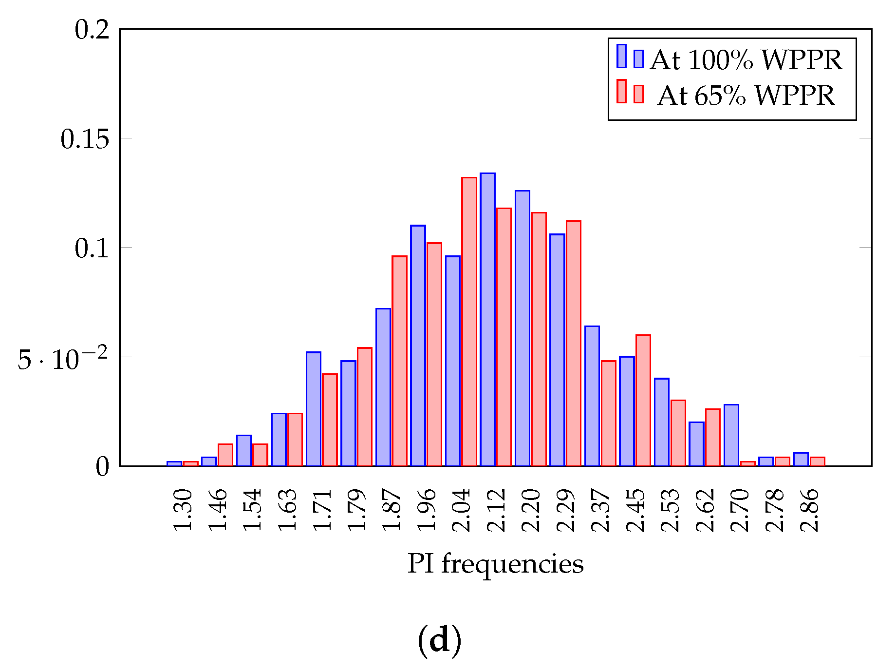
3.1.4. Profitability Index (PI)

PI also known as the benefit-cost ratio for project investment, is defined as the present value of the future cash flows divided by the initial investment. An investment is acceptable if its PI is greater than one. PI is calculated according to the following expression:

$$PI=\frac{{\sum }_{t=1}^n\frac{A_t}{{(1+r)}^t}}{I}=\frac{NPV}{I}+1$$

(17)

3.1.5. Levelized Cost of Energy (LCOE)

It measures lifetime costs of power generation technology per unit of electricity. The discounted cost of an investment project, also called the net present cost (NPC), is the present value of the sequence of cash inflows associated with the project minus the present value of all costs of installing and operating each component in the system over the project lifetime. It includes the investment, O&M and fuel expenditures at year t [17,18].

Since the principle of time value of money applies also to energy, the energy produced at a certain point in time has more value than if produced later. LCOE is calculated as the ratio of lifetime costs divided by the lifetime electricity generated by the hybrid system, both discounted back to a common year using a discount rate (see Equation (18)).

$$LCOE=\frac{NPC}{{\sum }_{t=1}^n\frac{E_t}{{(1+r)}^t}}=\frac{{\sum }_{t=1}^n\frac{C_t}{{(1+r)}^t}}{{\sum }_{t=1}^n\frac{E_t}{{(1+r)}^t}}$$

(18)

where $C_t$ is the outflow (sum of all costs) at year t, r is the discount rate and $E_t$ is the energy generated at year t.

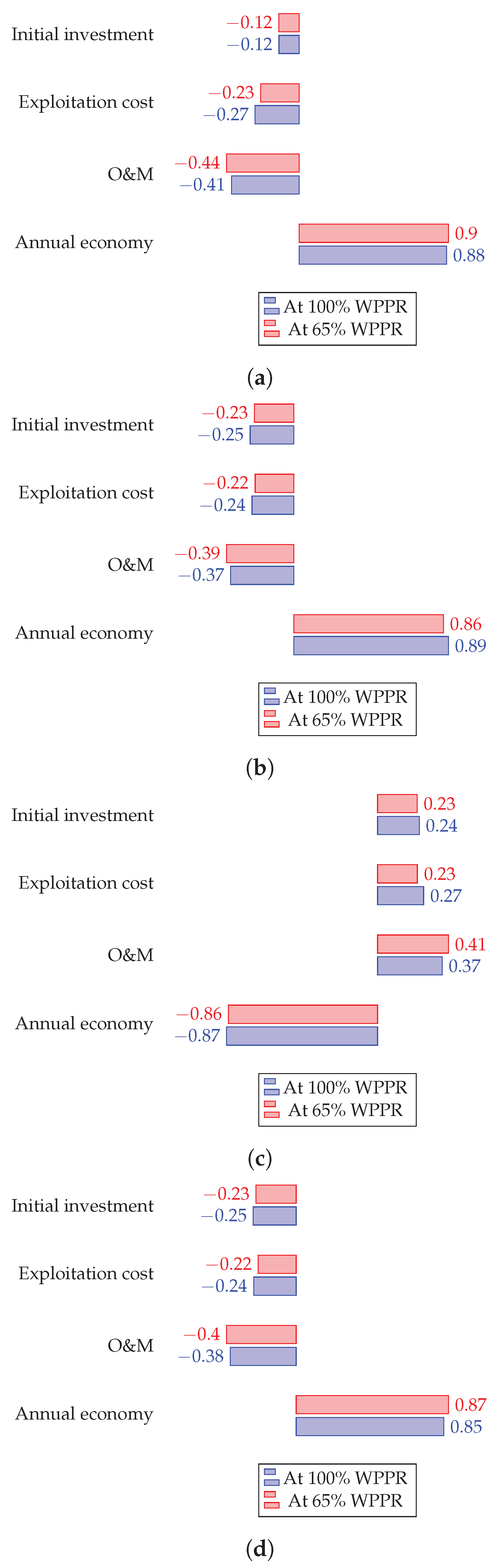
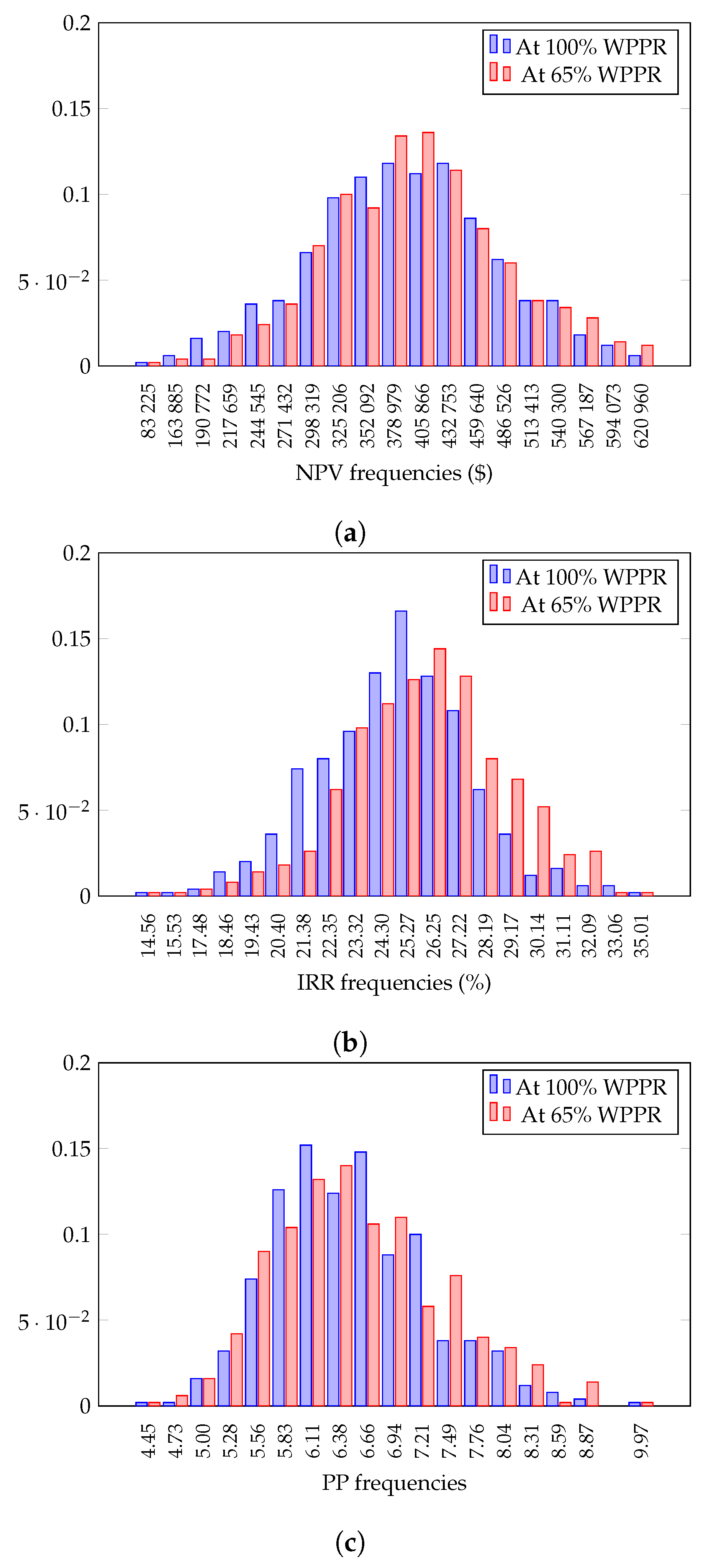
3.2. Risk Analysis

This module evaluates the robustness of the developed mathematical model by conducting a sensitivity analysis over a range of inputs parameters such as initial capital, project lifetime, cash flow and discount rate. The main interest is to determine the impact of such variations on NPV, IRR, PP and PI. The risk analysis model embedded within the WDCAS software is based on Monte Carlo simulations to assign probability distribution functions to each input variable.

Assume that each financial indicator F is a function of the vector of parameters $X=\left(x_1,x_2,x_3,x_4\right)$ in the form $F\left(X\right)$. A one-dimensional analysis is performed by creating a vector A composed of five feature values reflecting the impact on each term $x_i$ of $F\left(X\right)$. The impact is expressed according to a variation v over the range $-\frac{v}{2}$, $-\frac{v}{4}$, 0, $\frac{v}{4}$ and $\frac{v}{2}$. The variation v can be translated as $r_i=\frac{i-3}{4}v$, where i varies from one to five. Thus, the vector A can be mathematically expressed as:

$$A_i=F\left(x_i\left(1+r_i\right),x_j,x_p,x_q\right)$$

(19)

where i varies from one to five while $x_j$, $x_p$, $x_q$ parameters remain fixed. The impact of each variation of $x_i$ on F is expressed as follows:

Variation	Result
$-{\displaystyle \frac{v}{2}}$	$F\left(x_i\left(1-{\displaystyle \frac{v}{2}}\right),x_j,x_p,x_q\right)$
$-{\displaystyle \frac{v}{4}}$	$F\left(x_i\left(1-{\displaystyle \frac{v}{4}}\right),x_j,x_p,x_q\right)$
0	$F\left(x_i,x_j,x_p,x_q\right)$
${\displaystyle \frac{v}{4}}$	$F\left(x_i\left(1+{\displaystyle \frac{v}{4}}\right),x_j,x_p,x_q\right)$
${\displaystyle \frac{v}{2}}$	$F\left(x_i\left(1+{\displaystyle \frac{v}{2}}\right),x_j,x_p,x_q\right)$

A two-dimensional analysis is performed by creating a matrix B of size five by five. It reflects the combined impact of the variation of each pair $x_i$ and $x_j$ on F. The impact is expressed according to a variation v over the range $-\frac{v}{2}$, $-\frac{v}{4}$, 0, $\frac{v}{4}$ and $\frac{v}{2}$. The variation v can be translated as $r_i=\frac{i-3}{4}v$, where i varies from one to five for two parameters simultaneously. Thus, the elements of the matrix B are:

$$B_{ij}=F\left(x_i\left(1+r_i\right),x_j\left(1+r_j\right),x_p,x_q\right)$$

(20)

With the index $i,j$ varying from one to five, while $x_p,x_q$ remain fixed. The impact is expressed according to a variation v in the form of matrix B, as follows:

Variation	Result
$-{\displaystyle \frac{v}{2}}$	$B_{11}$	$B_{12}$	$B_{13}$	$B_{14}$	$B_{15}$
$-{\displaystyle \frac{v}{4}}$	$B_{21}$	$B_{22}$	$B_{32}$	$B_{42}$	$B_{52}$
0	$B_{31}$	$B_{23}$	$B_{33}$	$B_{43}$	$B_{53}$
${\displaystyle \frac{v}{4}}$	$B_{41}$	$B_{24}$	$B_{34}$	$B_{44}$	$B_{54}$
${\displaystyle \frac{v}{2}}$	$B_{51}$	$B_{25}$	$B_{35}$	$B_{45}$	$B_{55}$

The code generates a sequence of m numbers according to the normal probability distribution and the standard deviation range from $\frac{1}{3}$ to $m\sim N\left(0,\frac{1}{3}\right)$. The risk of a variation $r_i$ in a parameter $x_i$ is considered and then multiplied by the corresponding value of m. By default, m is set to be 500.

$$R_i=r_{i}m$$

(21)

Then, the financial indicator is calculated with respect to the new set of parameters:

$$F\left(x_i\left(1+R_i\right),x_j,x_p,x_q\right)$$

(22)

Finally, the risk analysis includes a diagram to visualize the impact of certain parameter on a particular financial indicator. The financial indicator F is subjected to a multi-linear regression based on the least square method. The resulting expression is presented in Equation (23).

$$\overline{F}\left(X\right)=\sum _{i=1}^4{\alpha }_i{x}_i+\epsilon$$

(23)

where ${\alpha }_i$ represents the slope of each simulation point, $\epsilon$ is the error due to the regression, $x_i$ corresponds to the financial parameter and $\overline{F}$ is the regressed financial indicator. The impact ${\gamma }_i$ in percentage terms can be represented by the contribution of each regressed parameter within the total variation, as follows:

$${\gamma }_i={\displaystyle \frac{{\alpha }_i{x}_i}{\overline{F}\left(X\right)}}$$

(24)

A series of Monte Carlo simulations has been carried out to analyze the impact ${\beta }_i$ of generated $x_i$ values on $\overline{F}\left(X\right)$. ${\beta }_i$ measures the impact more precisely since it deals with data resulting from a probability distribution. Ultimately, ${\beta }_i$ values are plotted to obtain an impact diagram.

$${\beta }_i={\displaystyle \frac{{\alpha }_i{\sigma }_i}{{\sigma }_F}}$$

(25)

where ${\sigma }_i$ is the standard deviation of the inputs $x_i$ and ${\sigma }_F$ is the standard deviation of the result given by Equation (25).

In complement to this set of relations, the median and the confidence interval are calculated for each financial indicator. The median is obtained directly from the Monte Carlo simulations. The confidence interval $\xi$ estimates the area of uncertainty related to the risk assessment of the project itself, the lower limit of confidence is the $\xi -th$ percentile and the upper limit is $\left(1-\xi \right)-th$ percentile of the series.

3.3. Environmental Analysis

This module quantifies the number of tons of ${\mathrm{CO}}_2$ emitted by the system. It also compares different system configurations and evaluates the profit associated with ${\mathrm{CO}}_2$ emission reduction. ${\mathrm{CO}}_2$ emissions can be calculated by using Equation (26).

$$e_{C{O}_2}=E_{system}{f}_{C{O}_2}$$

(26)

where $e_{C{O}_2}$ is the ${\mathrm{CO}}_2$ emission in $\mathrm{kg}{\mathrm{CO}}_2$, $E_{system}$ is the energy produced by the system in kWh and $f_{C{O}_2}$ is the emission factor in $\mathrm{kg}{\mathrm{CO}}_2·{\mathrm{kWh}}^{-1}$.

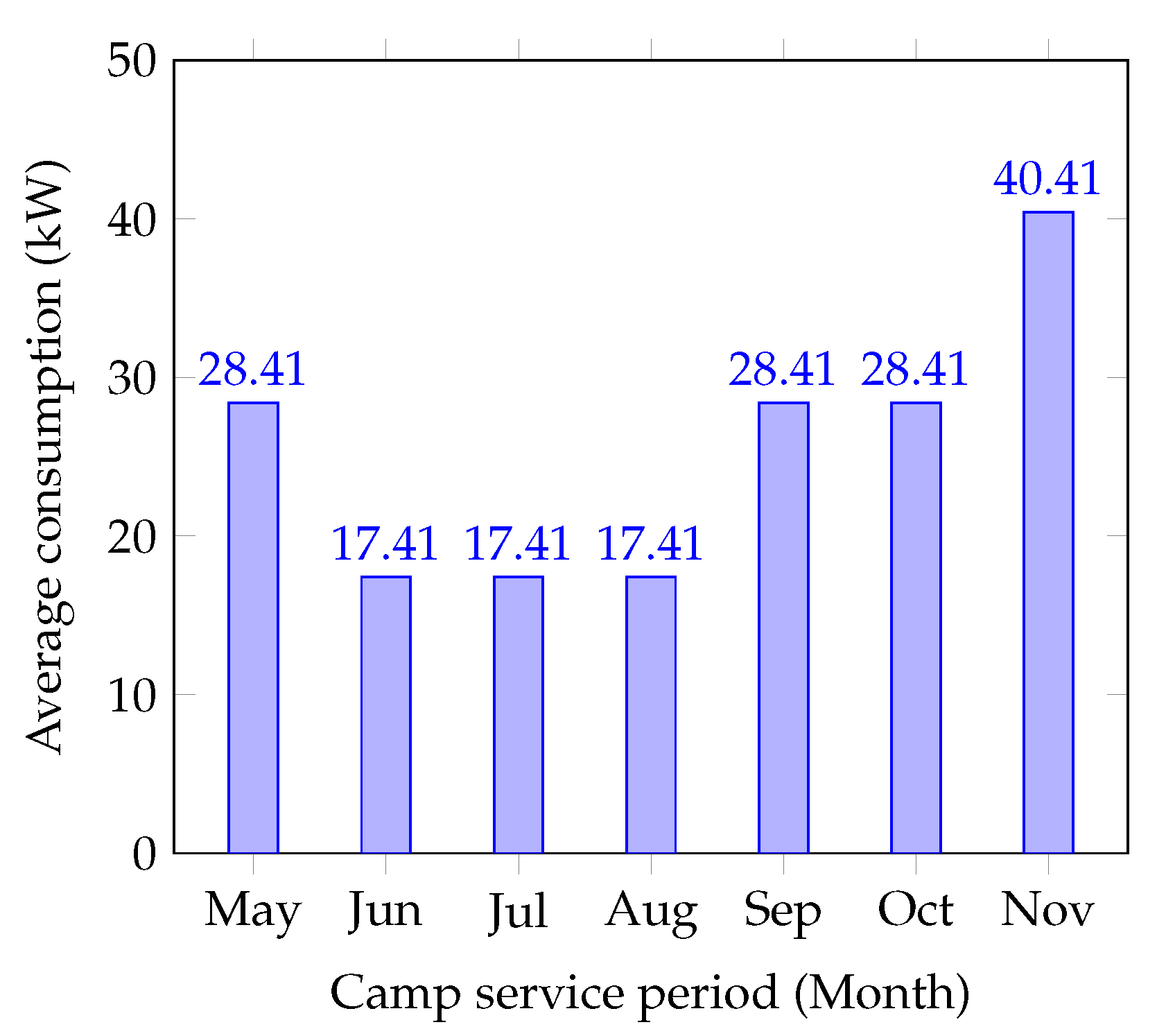
3.4. Case Study

The data for the case study corresponds to a mining camp located in a remote area in Newfoundland and Labrador, Canada. This site belongs to a company providing rail transportation services between the cities of Sept-Îles and Schefferville in Northern Quebec. The camp is open seven months per year, from May to November and it is unconnected to the main grid. Energy consumption varies according to daytime and season, the main loads are for lighting, heating, auxiliary equipment and water pumping station.

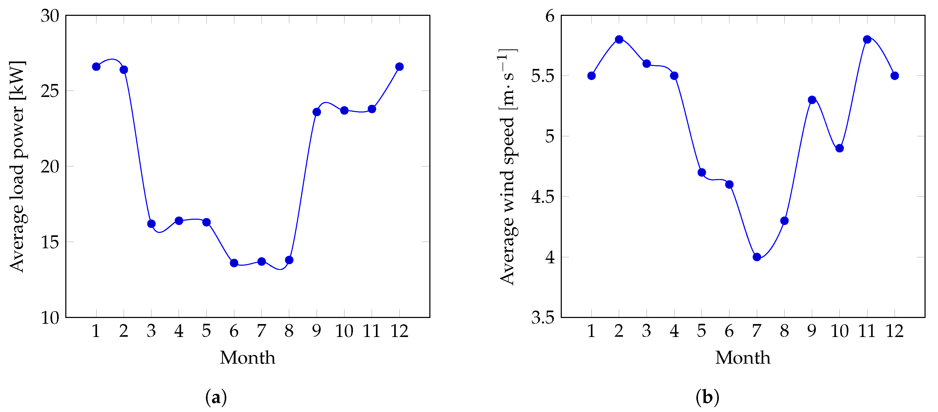
Figure 2 shows load and wind speed data under study. Figure 2a illustrates the annual average load profile of Esker camp. Real power data is obtained directly from the stand-alone hybrid system. The average load power is 19.9 kW, the lowest and upper consumption levels are 7 kW and 50 kW, respectively. These values determine the wind–diesel system configuration used for comparison. Figure 2b illustrates the monthly average wind speed data obtained from Environment Canada in a neighboring site of Esker camp. The annual average wind speed at 10 m above ground level is $5.1{\mathrm{m}·\mathrm{s}}^{-1}$. As wind speed probability distribution values are unknown, a Weibull probability distribution with a shape parameter of two (Rayleigh distribution) is considered.

4. Results and Discussion

4.1. WDCAS, HOMER and RETScreen Software Comparison for a Wind–Diesel Hybrid System

In this section, results of financial, risk and environmental analysis obtained from WDCAS, HOMER and RETScreen software are compared for a given wind-diesel hybrid system. According to Reference [19], diesel engine and WT lifespan is 15,000 h and 15 years respectively. WT replacement cost corresponds to the initial cost once its lifetime expires. Diesel engine replacement cost corresponds to the initial cost multiplied by the annual usage ratio, for example, the annual operating hours divided by the lifespan. The hourly maintenance is estimated to 0.001% of the diesel engine’s initial cost, the annual O&M of WT is estimated as 3% of the initial cost and the project lifetime is 20 years.

Table 1. Wind–diesel hybrid system configuration and equipment related costs.

Equipment	System Configuration		Equipment Related Costs ($)
	Quantity	Type	Unit Price	Initial Capital	O&M
Diesel generator	5 × 12 kW	D13-2 Caterpillar	8400	42,000	7105
WT at 40% WPPR	2 × 10 kW	BWC Excel-S Bergey	100,000	200,000	6000
Cost summary				242,000	13,105

summarizes the system configuration and the total associated cost of each equipment component including shipping and commissioning. The cost of producing electricity on site is estimated at $1.31\${\mathrm{kWh}}^{-1}$. This amount can be used as reference to determine the equivalent annual revenues associated with the wind–diesel hybrid system (244,254 $). The fuel price and the associated fuel procurement cost is estimated at 2.5 $ per liter according to the expected global rise of fossil fuels, as mentioned in Reference [18]. As result, the annual fuel cost is obtained from the multiplication of the fuel price and the fuel annual consumption (56,321 L), it means 140,803 $ at a discount rate of 6%.

4.1.1. Financial Analysis

Financial analysis is performed using WDCAS, HOMER and RETScreen software. The comparison is made based on relevant financial indicators such as NPC, LCOE, NPV, IRR, PP and PI. Simulations results are presented in

Table 2. Financial indicators comparison between HOMER and WDCAS software.

Financial Indicator	HOMER	WDCAS	Error (%)
NPC ($)	2,445,924	2,487,817	1.71
LCOE ($ ${\mathrm{kWh}}^{-1}$)	1.10	1.17	5.89
Annual energy produced (kWh)	174,687	186,220	6.60

and

Table 3. Financial indicators comparison between RETScreen and WDCAS software.

Financial Indicator	RETScreen	WDCAS	Error (%)
NPV ($)	222,300	219,039	1.47
IRR (%)	15.80	16.00	1.98
PP	6.00	5.60	5.82
PI	1.90	1.91	0.70

.

Table 2 shows that the NPC error is small compared to the cost of energy and the annual energy produced. One reason for the discrepancy in the error might be that the operating strategies are not identical between both software (e.g., time delays in switching among power sources, commutation errors associated when using a specific diesel generator, etc.). From Table 3 it is possible to observe that in most cases the error is less than 2%, this approximation validates the accuracy of the proposed computer model. Results concerning payback period indicator suggest that the discrepancy in the error might be due to rounding adjustment set by RETScreen software itself.

4.1.2. Sensitivity Analysis

Based on the case study, a sensitivity analysis is carried out to evaluate the robustness of the proposed computer model. A range of estimates of the initial investment and the cash flow is provided to determine whether such variations result in NPV optimization.

Simulation results by using RETScreen and WDCAS are shown in the

Table 4. RETScreen software sensitivity analysis.

	Initial Capital	217,800 $	229,900 $	242,000 $	254,100 $	266,200 $
Cashflow	Variation	−10%	−5%	0%	5%	10%
36,475 $	−10%	177,840 $	153,640 $	129,440 $	105,240 $	81,040 $
38,502 $	−5%	224,270 $	200,070 $	175,870 $	151,670 $	127,470 $
40,528 $	0%	270,700 $	246,500 $	222,300 $	198,100 $	173,900 $
42,554 $	5%	317,130 $	292,930 $	268,730 $	244,530 $	220,330 $
44,581 $	10%	363,560 $	339,360 $	315,160 $	290,960 $	266,760 $

and

Table 5. WDCAS software sensitivity analysis.

	Initial Capital	217,800 $	229,900 $	242,000 $	254,100 $	266,200 $
Cashflow	Variation	−10%	−5%	0%	5%	10%
36,434 $	−10%	177,858 $	153,658 $	129,458 $	105,258 $	81,058 $
38,458 $	−5%	224,291 $	200,091 $	175,891 $	151,691 $	127,491 $
40,482 $	0%	270,723 $	246,523 $	222,323 $	198,123 $	173,923 $
42,506 $	5%	317,155 $	292,955 $	268,755 $	244,555 $	220,355 $
44,530 $	10%	363,587 $	339,387 $	315,187 $	290,987 $	266,787 $

, respectively. Given the initial investment of 242,000 $ and the annual average cash flow of 40,528 $ for RETScreen (this value contains a rounding error of 0.1%) and 40,482 $ for WDCAS (average of the annual revenues from selling the energy at $1.31\${\mathrm{kWh}}^{-1}$ minus the expenses associated with fuel, O&M, equipment replacement and operating costs for the project lifetime of 20 years), the obtained NPV values are presented in a matrix format considering that the range of estimates is subjected to a variation of 10% with an increment of 5%. In this case, the sensitivity analysis has been implemented in which the average error in the matrix of differences between RETScreen and WDCAS was about 0.01%. Thus, the results demonstrate the effectiveness of the proposed WDCAS software.

4.1.3. Risk Analysis

In this section a quantitative risk analysis is implemented. The purpose is to determine the influence of each financial indicator on the NPV. The initial investment, the revenues and the expenses are considered as inputs. The risk analysis operates as a sensitivity analysis in which the inputs are not fixed; the range of input estimates is subjected to a variation of 10% and follows a normal distribution bounded by a maximum. Each time a random number is generated, the inputs are computed and then a linear regression is applied to estimate the NPV. The simulation results are presented in

Table 6. Impact of input variables on the net present value by using RETScreen and WDCAS software.

Input Variable	RETScreen	WDCAS	Error (%)
Initial investment	−0.07	−0.08	16.02
Revenues	0.74	0.84	13.66
Expenses	−0.62	−0.75	20.01

.

The revenues are considered as the most influence indicator on the NPV. The NPV median values calculated by using RETScreen and WDCAS software were 219,787 $ and 233,198 $ respectively, with an error of 6.10%. However, error measurements between both software are subjected to the number of iterations conducted.

4.1.4. Environmental Analysis

${\mathrm{CO}}_2$ emission is used as indicator to assess the environmental impact of using a wind–diesel hybrid system. The tons of ${\mathrm{CO}}_2$ emissions calculated using RETScreen and WDCAS software were 122.07 and 122.44 respectively. According to RETScreen software documentation, the diesel emission factor is assumed of 0.833 Kg ${\mathrm{CO}}_2{\mathrm{kWh}}^{-1}$. The same factor is used in WDCAS software to calculate the quantity of ${\mathrm{CO}}_2$ emitted by the wind–diesel hybrid system. It is also assumed that wind energy systems do not produce GHG emissions. As a result, the total energy produced by diesel generators is 84% of 186 MWh, approximately 156 MWh. Finally, an error of 0.30% is obtained by comparing the results of both software.

4.2. WDCAS Software Validation for a Wind–Diesel Hybrid System with Compressed Air Energy Storage

In this section, the WDCAS software is used to assess the performance of a wind–diesel hybrid system with compressed air energy storage. The data presented in the case study of the Section 3.4 is used to evaluate the feasibility of the proposed hybrid system. Figure 3 illustrates the average consumption profile of Esker camp in 2014. As mentioned before, the site operates seven months per year and produces its own electricity. Currently, a diesel generator of 150 kW provides power when needed. The main loads are for lighting, heating, auxiliary equipment and water pumping station. The annual fuel consumption of the current system is about 112,420 L which represents an annual cost of 281,050 $ for a fuel cost of $2.5\${\mathrm{L}}^{-1}$. From a technical point of view, the diesel generator is oversized considering the energy consumption of the site; most of the time it operates with low efficiency which causes excess fuel consumption. Furthermore, when the system fails, a diesel generator of 6.5 kW acts as backup unit. However, it is not enough to satisfy the power demand.

By using load and wind speed data, WDCAS software calculates the optimal system configuration. It also determines time and frequency of operation for each power source, fuel consumption and energy dissipation. In this case, the proposed solution is composed of two diesel generators of 27 kW Model D30-8 Caterpillar and a WT BWC Excel-S Bergey. At 65% and 100% WPPR, the hybrid system uses four and five wind turbines respectively.

Table 7. Wind–diesel hybrid system with compressed air energy storage configuration.

Equipment	Power Data Equipment	Details
Diesel generator	2 × 27 kW	D30-8 Caterpillar
WT at 65% WPPR	4 × 10 kW
WT at 100% WPPR	5 × 10 kW	BWC Excel-S Bergey

summarizes the data obtained from simulation.

Additional simulations are carried out to determine the system performance improvements by adding CAES. The following assumptions characterize the operating strategy:

• Assuming ideal conditions, there is not limit on the required storage capacity of the tank.
• The overall power dissipated by the ESS is null, it means that the excess of power is used by the storage unit.
• The power losses are diminished since motor/compressor efficiency is 90%, as well as the mechanical losses as polytropic efficiency is 80%.
• Compression performance improvement is achieved when increasing the number of compressor stages.
• The compression is done under the following conditions: the outdoor air pressure is equal to 1 bar, the storage temperature is set at 20 °C and the polytropic exponent of air at room temperature is $n_c=1.3$.

In accordance with the above-mentioned points, model input parameters are presented in

Table 8. WDCAS model input parameters.

Parameter	Symbol	Value
Number of compressor stages	$N_C$	5
Polytropic index	$n_c$	1.3
Atmospheric pressure	$p_a$	1 bar
Storage temperature	$T_{st}$	20 °C
Polytropic efficiency	${\eta }_{p_C}$	80%
Compressor motor efficiency	${\eta }_{tr}$	90%
Minimum required power for storage	$P_{CAE{S}_{min}}$	5 kW
Storage pressure	$p_{st}$	30 bars
Number of days of autonomy	$N{D}_{auto}$	1000

. The obtained results from these configurations are illustrated in Figure 4. The baseline diesel only configuration is used as reference to compare the performance of the proposed WDCAS operating at 65% and 100% WPPR.

As Figure 4 indicates, the diesel only operating mode requires 112,420 L of fuel per year comparing with 35,917 L and 33,851 L required by the WDCAS operating at 65% and 100% WPPR respectively. Thus, fuel savings up to 68.1% and 69.9% are obtained by using the WDCAS instead of the baseline configuration with a 150 kW diesel generator. Adding CAES to the hybrid system significantly reduce the number of hours and the dissipated energy during which diesel generator is operating.

An increase on the number of WT does not provide a significant gain in time at 100% WPPR, less than 10% gain is achieved for a supercharged and no supercharged diesel engine. This can be explained by the fact that wind speed on this area is not powerful enough. Furthermore, a difference of 18% between the dissipated energy is observed when comparing WDCAS configurations at 65% and 100% WPPR.

4.2.1. Financial Analysis

The cost data for each subsystem is presented in

Table 9. Influence of WPPR on fuel economy, diesel generator and wind turbine (WT) costs.

Financial Indicator	At 65% WPPR	At 100% WPPR	Difference (%)
Fuel Economy
Fuel cost ($)	89,793	84,627	6.00
Annual fuel economy ($)	191,258	196,423	3.00
Diesel Generator
Initial Capital ($)	37,800	37,800	-
Financial depreciation ($)	15,057	15,034	0.15
O&M ($)	2259	2255	0.15
WT
Total Capital ($)	400,000	500,000	25.00
Financial depreciation ($)	26,667	33,333	25.00
O&M ($)	1200	1500	25.00

. The data provided is used in the economic model to determine the profitability of the hybrid system. For instance, the fuel cost decreases by 6% when the hybrid system operates at 100% WPPR. The annual fuel economy is estimated at 3% when comparing the WDCAS technology at 65% and 100% WPPR and no significant gain is observed for further increasing the number of WT.

The diesel generator total cost is estimated based on market prices. The annual depreciation is expressed as the initial cost multiplied by the annual usage ratio, for example, the annual operating hours divided by the lifespan of 15,000 h [12]. Resulting O&M costs are computed annually over the expected life of the diesel engine, the maintenance cost is calculated as 0.001% of the initial cost per operating hours [12]. As referred previously, increase the number of WT does not provide a significant gain in terms of financial depreciation at 100% WPPR.

The WDCAS software sizes the WT according to the wind profile, the geographical location and the electrical power demand. The total cost of the WT is distributed between the initial acquisition, transportation and installation as well as the on-going maintenance. The WT lifetime is estimated to 15 years [16], therefore the depreciation is equivalent to the ratio of the total cost to the lifetime. In addition, the O&M cost is estimated to be 3% of the initial cost [16].

The WDCAS software sizes the CAES system according to the quantity of airflow eventually required by the wind–diesel hybrid system operation. The firm that designed the CAES system estimated the price to be $\mathrm{50,000}\${\mathrm{m}}^{-3}$. The control room cost includes the total price of the building and the control equipment. The lifetime of the ESS is estimated to 20 years and the O&M cost is estimated to 1% of the total initial cost. In this case study, the total cost of the ESS is covered from the beginning of the project.

A summary of the main costs incurred by the implantation of the WDCAS is presented in

Table 10. Cost summary at 65% and 100% WPPR.

Financial Indicator	Amount at 65% WPPR	Amount at 100% WPPR	Difference (%)
Initial capital ($)	322,000	322,000	-
Financial depreciation ($)	41,724	48,368	16.00
O&M ($)	6329	6625	5.00
Exploitation cost ($)	89,793	84,627	6.00
Annual fees ($)	137,845	139,620	1.00
Annual economy ($)	191,258	196,423	3.00

. It contains the initial capital, the annual fees and the annual economy. The depreciation, the O&M and the exploitation cost in terms of fuel are considered as part of the annual fees. Finally, the annual economy is viewed as revenue for future financial computations, sensitivity and risk analysis. The initial capital is chosen to be the same at 65% and 100% WPPR as the ESS have been paid at the beginning of the project. The financial depreciation increases close to 16% with the addition of the WT. The O&M costs increase by 5%, the exploitation cost dropped by 6% as consequence of a reduction in fuel consumption. Finally, the annual fees and the annual savings increased by 1% and 3% respectively, thanks to the drop-in fuel consumption.

The discounted cash flow is another indicator to include in the financial analysis. It allows an evaluation of the future net cash flow using present values, it can be calculated as the NPV in which the discount rate is chose to 10% and the fuel index rate is estimated to 5%. Figure 5 illustrates the discounted cash flow over the life cycle of the project, it gives an idea of the profitability derived from the use of WDCAS. All discounted cash flow based on a discount rate of 10% per year in a period of 20 years reflects a difference equal to 6% between the two levels of WPPR. Since the index rate is the same, the difference is related to the cash flow statement itself. An increase of 5% is observed in cash flow for the WDCAS operating at 100% WPPR. It is concluded that at both scenarios, the cash flow remains positive through the project life cycle.

As can be seen from

Table 11. Summary of key indicators used in the financial analysis.

Financial Indicator	Amount at 65% WPPR	Amount at 100% WPPR	Difference (%)
NPV ($)	357,287	400,399	12.00
IRR (%)	21.00	23.00	6.00
PI	2.11	2.24	6.00
Discounted payback	7.88	7.38	6.00
Annual energy production (kWh)	222,154	222,154	-
Energy production over 20 years (kWh)	4,443,072	4,443,072	-
NPC ($)	1,475,060	1,489,911	1.00
LCOE ($\${\mathrm{kWh}}^{-1}$)	0.78	0.79	1.00

, the NPV is the total discounted cash flow. The IRR is the maximum discount rate consistent with a profitable project and is larger than the discount rate of 10%. The PI describes the efficiency of the project. In the context of the case study, the PI is superior to one; it means that the overall profit is superior to the overall expenses. At 100% WPPR, the NPV increases by 12%, the IRR and the PI increase by 6%, all of them as consequence of an increase in the annual economy. The payback corresponds to the number of years required to pay all the expenses of the project and the discounted payback can be viewed as the duration needed for the project to start making positive cash flow. As mentioned before, the cash flow is higher at 100% WPPR, thus it declines the discounted payback as well. The NPC is the total discounted outflow, it is used to compute the energy cost. The latter is defined as the net present cost divided by the total discounted energy produced during the project life cycle. At 100% WPPR, for the same energy produced, the wind turbine O&M and depreciation costs influence the rise of the NPC and the LCOE by 1%. In diesel only operation mode the LCOE is equal to $1.27\${\mathrm{kWh}}^{-1}$. At 65% WPPR, the LCOE is equal to $0.78\${\mathrm{kWh}}^{-1}$ and at 100% WPPR the LCOE is $0.79\${\mathrm{kWh}}^{-1}$, then the energy cost is reduced by 39% and 38% when using WDCAS technology. This can be explained by the energy management strategy used which promotes a reduction of fuel consumption in diesel engine.

4.2.2. Sensitivity Analysis

Simulation results evaluating the influence of the initial investment, the exploitation cost, the O&M and the annual economy on NPV, IRR, PP and PI are presented in Figure 6.

According to the range of values in Figure 6a, the NPV impact diagram resulting from the WDCAS software indicates that the annual economy predominated as the most influential factor against the initial investment, the exploitation cost and the O&M. The sensitivity analysis estimates 89% and 88% of the annual economy at 65% and 100% WPPR, respectively. The initial investment is equal to −12% at both values of WPPR. The exploitation cost has an impact of −23% at 65% WPPR and −26% at 100%, it means a difference of 14%. The O&M impact in percentage is equal to −44% at 65% WPPR and −41% at 100% WPPR representing a difference of 7%.

The impact diagram presented in Figure 6b indicates that the annual economy predominated as the most influential factor on the IRR against the initial investment, the exploitation cost and the O&M. The sensitivity analysis estimates 86% and 89% of the annual economy at 65% and 100% WPPR, respectively. The initial investment is equal to −23% at 65% WPPR and −25% at 100% WPPR, 11% of difference between both WPPR values. The exploitation cost has an impact of −22% at 65% WPPR and −24% at 100%, it means a difference of 8%. The O&M impact in percentage is equal to −39% at 65% WPPR and −37% at 100% WPPR representing a difference of 6%.

The diagram impact obtained from the payback period is shown in Figure 6c. The annual economy predominated as the most influential factor against the initial investment, the exploitation cost and the O&M. The sensitivity analysis estimates −86% and −87% of the annual economy at 65% and 100% WPPR, respectively. The initial investment has an impact of 23% and 24% on the PP, 6% of difference between both WPPR values. The exploitation cost has an impact of 23% and 27% at 65% and 100% WPPR, it means a difference of 15% between both WPPR values. The O&M impact in percentage is equal is 41% at 65% WPPR and 37% at 100% WPPR. A difference of 9% between the two values of WPPR.

The diagram impact obtained from the profitability index is shown in Figure 6d. The annual economy predominated as the most influential factor against the initial investment, the exploitation cost and the O&M. The sensitivity analysis estimates 87% and 85% of the annual economy at 65% and 100% WPPR, respectively. The initial investment has an impact of −23% and −25% on the PI, 7% of difference between both WPPR values. The exploitation cost −22% and −24% at 65% and 100% WPPR, it means a difference of 12% between both WPPR values. The O&M impact percentage for PI is −40% at 65% WPPR and −38% at 100% WPPR. A difference of 5% between the two values of WPPR.

From this, it can be concluded that the operating cost impacts are small at low penetration levels and moderate at higher WPPR. The influence between both WPPR values on each financial indicator shows slight fluctuations. The use of CAES reduces the exploitation costs by decreasing fuel consumption allows an increase of the annual economies and the energy efficiency of the hybrid system. Similarly, O&M costs can be significantly reduced by applying an effective predictive maintenance strategy. The discrepancies between the defined WPPR values are negligible and exhibit the same behavior. Since IRR impact diagram also exhibits similar behavior as for the NPV impact diagram, by extension the same recommendations apply. The rank of the PP impact remains unchanged in this chart for the payback. The difference translates the effect of the added wind turbine in the initial investment and the fuel consumption for the O&M with exploitation cost.

4.2.3. Risk Analysis

In this section a risk analysis is conducted to assess the role of NPV, IRR, PP and PI. The expected value of the probability distribution for each financial indicator is obtained from Monte-Carlo method and illustrated in Figure 7. A risk rate of 15% is used when executing simulations. The confidence interval and the median are calculated using the WDCAS software, these values are summarized in

Table 12. Financial indicators statistics at 65% and 100% WPPR.

Operating Strategy	Median	Lower Limit Confidence Interval	Upper Limit Confidence Interval	Average
NPV ($)
At 65% WPPR	354,796	236,847	493,761	357,518
At 100% WPPR	411,243	274,152	543,687	409,252
Difference (%)	16.00	16.00	10.00	14.00
IRR (%)
At 65% WPPR	22.34	18.25	26.56	22.28
At 100% WPPR	23.56	19.39	27.36	23.43
Difference (%)	5.00	6.00	3.00	5.00
PP
At 65% WPPR	6.03	5.06	7.51	6.15
At 100% WPPR	5.71	4.80	7.05	5.78
Difference (%)	5.00	5.00	6.00	6.00
PI
At 65% WPPR	1.97	1.59	2.35	1.97
At 100% WPPR	2.08	1.69	2.50	2.09
Difference (%)	6.00	6.00	7.00	6.00

.

The risk analysis provides an estimated NPV difference of about 14% between both WPPR values. The NPVs obtained were found in agreement with the results of the financial analysis. The confidence interval also contains the generated net present values as predicted previously. In the same way, the confidence interval contains the computed IRR as predicted for a risk rate of 15%. Finally, the median and the average is also close to the actual IRR in both WPPRs. The average difference in the results is close to 5%, it is the same variability previously computed. The median and the average of the payback period is close to 6%. The confidence interval about the PP describes the statistical prediction based on a range of estimates yielding a risk rate of 15%. The resulted difference in the risk analysis is compatible with the computed values obtained in the financial analysis. The average and the median profitability index for both WPPRs are close to the expected PI value bounded by the confidence interval required for a risk rate of 15%. The average difference in the results is about 6%, these observations fit with the previously computed variability. As a conclusion, the risk analysis offers a more realistic forecast of financial indicators to help the decision-making process.

4.2.4. Environmental Analysis

Table 13. Environmental impact of using WDCAS.

Operating Strategy	Energy (kWh)	Tons of ${\mathbf{CO}}_2$ Emissions Produced	Difference (%)
Diesel only	134,771	34.10	-
WDCAS at 65% WPPR	107,519	27.20	20.00
WDCAS at 100% WPPR	102,178	25.90	24.00

compares the environmental impact of replacing diesel engine with WDCAS technology. The use of WDCAS leads to a reduction of GHG emissions by 20% and 24% at both values of WPPR compared with the baseline diesel only configuration.

5. Conclusions

In this paper, a computer model for financial, environmental and risk analysis has been developed for a wind–diesel hybrid system with compressed air storage. First, the model has been validated by comparing a wind–diesel case study results against those obtained using HOMER and RETScreen software. Similar results were obtained by analyzing the impact on financial and environmental performances when using WDCAS software. Then, the proposed computer model has been applied to analyze the impact of adding compressed air energy storage on the wind–diesel hybrid system.

The use of wind–diesel power system associated with CAES appears as an optimal configuration to fulfil the needs of electrification in remote areas as the Esker mining camp in the northeastern province of Canada. One advantage of using the proposed software is that it allows to vary the size of all subsystems and to determine the design that provides optimal performance, through a general interface and based on a variety of results, respectively. Despite a non-optimal WPPR, significant economic savings can be obtained through the use of compressed air. Although a high initial capital investment is required, the proposed solution may not only reduce the exploitation of diesel engines in remote areas but also improve system life-cycle and reduce maintenance costs.