Hour-Ahead Solar Irradiance Forecasting Using Multivariate Gated Recurrent Units

Abstract

Variation in solar irradiance causes power generation fluctuations in solar power plants. Power grid operators need accurate irradiance forecasts to manage this variability. Many factors affect irradiance, including the time of year, weather and time of day. Cloud cover is one of the most important variables that affects solar power generation, but is also characterized by a high degree of variability and uncertainty. Deep learning methods have the ability to learn long-term dependencies within sequential data. We investigate the application of Gated Recurrent Units (GRU) to forecast solar irradiance and present the results of applying multivariate GRU to forecast hourly solar irradiance in Phoenix, Arizona. We compare and evaluate the performance of GRU against Long Short-Term Memory (LSTM) using strictly historical solar irradiance data as well as the addition of exogenous weather variables and cloud cover data. Based on our results, we found that the addition of exogenous weather variables and cloud cover data in both GRU and LSTM significantly improved forecasting accuracy, performing better than univariate and statistical models.

1. Introduction

In recent years, solar electricity has grown in popularity due to the lowering costs of manufacturing and the rising efficiency of solar panels. In order to fully integrate solar electricity into power grid systems, information regarding the amount of solar irradiance from the sun at a given location and future time period must be known to estimate the amount of electricity that will be generated and dispatch accordingly [1]. This can be a challenge for power grid operators given the stochastic nature of solar irradiance due to cloud cover, humidity, air temperature, and other environmental factors. Using accurate predictions of future solar irradiance values, power grid operators would be able to determine how much energy will be generated in the near future, dispatch power to supply electricity as needed, and schedule power generation to meet the varying demands of electricity throughout the year [1].

Global Horizontal Irradiance (GHI) is defined as the amount of solar irradiance hitting a surface horizontal to the Earth’s surface [2]. GHI is an important measurement for photovoltaic (PV) power plants, because it allows plant operators to estimate the amount of power generated at a given time and model PV performance over time. GHI can be measured using a pyranometer or calculated based on the Direct Normal Irradiance (DNI) and Diffuse Horizontal Irradiance (DHI), where DNI is the beam irradiance from the sun directly hitting the surface at a perpendicular angle and DHI is the surrounding irradiance that has been scattered by the Earth’s atmosphere coming from equal angles of the surface [2,3]. In non-concentrating PV power plants, forecasting future PV power production primarily utilizes GHI forecasts, while concentrated solar power forecasting can only benefit from forecasts of DNI [3]. The amount of GHI and DNI hitting the Earth’s surface is dependent on the amount of cloud cover over a particular site [3,4,5] as well as weather patterns in the area, such as air temperature, relative humidity, wind speed and direction, and dew point [2,6,7]. Forecasting GHI and PV power output are similar in that both depend on surrounding weather and cloud activity [8]. Using GHI forecasts and the characteristics of a particular PV panel, power production can be predicted for some time in the future to measure PV power plant performance and efficiency for PV installations [9,10]. In this paper, we forecast GHI rather than PV power production in order to compare our results to existing literature in forecasting solar irradiance.

Given the high degree of variability, forecasting solar irradiance has been largely studied in the literature in order to obtain higher prediction accuracy and more efficient modeling. Research efforts in forecasting solar irradiance include the use of physics, statistics, and machine learning models using cloud imagery, historical solar irradiance, and exogenous weather data to predict solar irradiance over short and long time horizons [1]. Physics-based models, including Numerical Weather Prediction (NWP) models, use satellite and ground-based sky image data to evaluate cloud formations and predict solar irradiance [11,12].While physics-based models explain causality through closed-form equations or numerical simulations, the solutions are in some cases limited with respect to their computational tractability [1]. On the other hand, statistics-based models, including Regression [13], Exponential Smoothing Models [14], and variants of the Autoregressive Integrated Moving Average (ARIMA) model [4,13,15], have been implemented for solar irradiance forecasting over shorter horizons. These models use statistical analysis in order to map inputs to the forecast variable; however, considering the non-stationary nature of solar irradiance data, statistical models fail to accurately predict sudden changes in solar irradiance [13]. Various operational decisions are often dependent on short- and long-term forecasts, where short-term forecasting refers to forecasts over one to six hours and long-term forecasting refers to predicting solar irradiance over six hours to a couple of days [1]. In practice, statistical models and forecasting models using satellite cloud imagery perform well for short-term forecasts [1,16]; these forecasts provide insight on how much solar power may be generated in the near future and influence intraday power scheduling decisions [14]. Conversely, physics-based models perform better for long-term forecasts which are used to develop plans for integrating solar power systems [16]. Multivariate time series models capture the influence of multiple variable on the target variable to improve forecasting performance. Many previous studies [4] have shown empirical relationship between various variables such as solar zenith angle, ambient temperature, cloud cover, humidity, and air temperature and irradiance. We chose to experiment with multivariate GRU to evaluate if the model is able to capture the dynamic dependencies of these variables on future irradiance.

Machine learning models including Artificial Neural Networks have the ability to train the model using historical solar irradiance data, exogenous meteorological data, or both to capture the stochasticity of solar irradiance data. Melzi et al. [15] compared the performance of several machine learning techniques to statistical models using previous hours of solar irradiance and previous days containing the same number of daylight hours in order to forecast hourly solar irradiance. They found that combining exogenous variables to solar irradiance data improved model performance. Li et al. [6] evaluated the use of Hidden Markov Models (HMM) and Support Vector Regression (SVR) to forecast short-term solar irradiance under different weather conditions. They used exogenous weather variables, such as relative humidity, air temperature, and wind speed, as observation states within their HMM and found that these variables had a large impact on future solar irradiance. Aguiar et al. [17] designed Artificial Neural Networks that used ground solar irradiance data along with solar radiation and Total Cloud Cover forecasts as inputs to the model. The best results of their study were obtained by combining exogenous satellite data and Total Cloud Cover data. Yang et al. [4] tested the application of three different forecasting methods using GHI, DNI, DHI and cloud cover. Moreover, the addition of cloud cover information was shown to significantly improve the accuracy of forecasting models. Additionally, hybrid models have been developed by combining machine learning techniques with physics- or statistics-based models to improve overall forecasting performance compared to using a single type of model [18,19]. Reikard [13] evaluated the performance of regression combined with neural networks and found that the hybrid model performed better than regression or neural networks alone. Ogliari et al. [20] proposed a mixed method containing a physical-neural network model and a five parameters model for forecasting future PV power production, where the combination of these two forecasting methods resulted in competitive forecasting 24 h in advance.

More recently, deep learning techniques have been utilized in solar irradiance and solar power production forecasting. Gated Recurrent Neural Networks (RNN) are a special type of deep learning model that have shown promising results in forecasting sequential data due to their ability to pass long-term information from previous computations as inputs [21]. Long Short-Term Memory (LSTM) and Gated Recurrent Units (GRU) are two gated RNNs that have been shown to perform well for many different problems in predictive analytics, including speech recognition and traffic prediction [22,23]. LSTM and GRU differ from one another by the number of gates within their architecture and the transfer of information. Some empirical research has been done to measure the performance of GRU compared to LSTM given their differences; however, more research is needed to determine which network is superior and the preference for one gated RNN over another is often dependent on the data set [24]. Alzahrani et al. [25] used deep neural networks, namely LSTM, to predict short-term solar irradiance using data collected every millisecond over a four day period. They found that LSTM outperformed other traditional machine learning methods including SVR and Feedforward Neural Networks (FFNN). Abdel-Nasser and Mahmoud [26] tested various LSTM architectures in order to forecast PV power production using historical data and concluded that LSTM is able to accurately learn complex patterns in PV power time series. Qing and Niu [7] propose the use of LSTM for hourly day-ahead solar irradiance prediction using weather forecasts of the same day as input. The weather variables include temperature, dew point, humidity, visibility, wind speed, and weather type. They found that the LSTM learning algorithm is more accurate than linear least squares regression and neural networks using the back propagation algorithm due to better generalization. Husein and Chung [27] proposed the use of LSTM for day-ahead solar irradiance forecasting using only exogenous features and compared their proposed model to FFNN. LSTM outperformed traditional FFNN in all tested locations chosen based on average climate, leading to an increase in energy savings. Kumar et al. [28] used LSTM and GRU in spark clusters for hyperparameter tuning to forecast short-term electric load in power grids. Sorkun et al. [29] investigated the use of univariate RNNs, namely LSTM and GRU, for one hour ahead solar irradiance time series forecasting. They found that LSTM and GRU outperformed traditional RNNs indicating that gated RNNs are competitive in solar irradiance forecasting, but using only historical solar irradiance with LSTM or GRU was not superior to one another. Wang et al. [8] implemented multivariate GRU networks on groups of training sets containing similar features in order to accurately forecast short-term PV power output. Their multivariate GRU network outperformed existing forecasting models due to the addition of highly-correlated features and splitting the training sets into groups using K-means methods. Through their analysis, they also found that GRU has an advantage over LSTM due to less training time over large data sets. Although literature for the application of LSTM and GRU exists for predicting PV power production, an experimental study comparing LSTM and GRU with and without exogenous weather and cloud cover data has not been conducted.

In this paper, we evaluate the application of multivariate GRU for solar irradiance forecasting and compared the proposed model with univariate and multivariate LSTM. To the best of our knowledge, GRU in combination with hourly exogenous weather and cloud cover data has not been applied to short-term solar irradiance forecasting. The key contributions of this paper are the following:

• Propose the application of multivariate GRU to forecast hourly solar irradiance in Phoenix, Arizona one to ten time steps ahead using historical solar irradiance and exogenous weather variables
• Assess the impact of adding exogenous weather variables, such as solar zenith angle, relative humidity, air temperature, and cloud cover, to LSTM and GRU networks
• Performance comparison of prediction accuracy and computation time between GRU and LSTM using various configurations (i.e., univariate, multivariate without cloud cover, and multivariate with cloud cover)

The rest of the paper is organized as follows: Section 2 gives a brief description of the proposed model and describes our experimental plan to evaluate univariate and multivariate GRU against univariate and multivariate LSTM. Section 3 provides a performance comparison of GRU to LSTM and discusses the experimental results. Section 4 concludes our research paper and provides a plan for future work in this research area.

2. Materials and Methodology

We designed a Gated Recurrent Unit (GRU) to forecast hourly solar irradiance using real-world solar irradiance data, exogenous meteorological variables, and cloud cover time series data. We provide an experimental plan for evaluating the proposed model against LSTM and existing literature in terms of accuracy and computation time.

2.1. Multivariate GRU

GRU was first proposed by Cho et al. [30] as a simpler RNN architecture compared to LSTM, resulting in easier computation and implementation. The GRU network consists of designing multiple cells that adaptively remember and forget information as new information is received [30]. The feedback loops of the GRU network are unrolled in time such that the output of a previous cell is used as input to the next cell in addition to the current input example. This key feature allows gated RNNs to accurately understand and predict sequential data over time. GRU cells are similarly configured to LSTM cells; however, since GRU cells contain only two gates compared to three gates in LSTM, GRU requires fewer computations overall [29]. GRU cells contain a reset (r) and update (u) gate, as shown in Figure 1. The update gate decides how much information will be remembered, while the reset gate determines whether new information will be added to the previous state [29]. GRU cells are maintained using the following equations:

$$\begin{array}{cc}\hfill r_i& =\sigma \left(W_i^r{x}_i+Z_i^r{h}_i^{t-1}\right)\hfill \end{array}$$

(1)

$$\begin{array}{cc}\hfill u_i& =\sigma \left(W_i^u{x}_i+Z_i^u{h}_i^{t-1}\right)\hfill \end{array}$$

(2)

$$\begin{array}{cc}\hfill {\widehat{h}}_i^t& =\sigma \left(W_i{x}_i+U_i(h_i^{t-1}*r_i)\right)\hfill \end{array}$$

(3)

$$\begin{array}{cc}\hfill h_i^t& =u_i{h}_i^{t-1}+(1-u_i){\widehat{h}}_i^t\hfill \end{array}$$

(4)

where i represents the i-th hidden unit, W, Z, and U are the trained weight matrices, x represents the time series input vector, $\sigma$ denotes the chosen activation function, t represents time, and $h^{t-1}$ represents the previous output. These formulas are similar to LSTM in nature and more explanation is given in [30].

Due to its ability to manage long-term dependencies in sequential data, GRU performs well for time series forecasting problems. The GRU cells within a network are trained by minimizing a specific cost function using Backpropagation Through Time. In our experiments, specific cost functions perform better for univariate and multivariate cases: minimizing the mean squared error for the univariate experiments and the mean absolute error for the multivariate cases resulted in better performance. To forecast the amount of solar irradiance at time t, the observations from T previous time steps are considered. In our case, we utilize the last $T=48$ time steps or hours in order to obtain the best results. In the univariate experiments, the GRU and LSTM networks contain one deep layer with 10 units; meanwhile, multivariate experiments contain three layers with 60, 30, and 10 units, respectively. We train the univariate models using 100 epochs, and multivariate models using 50 epochs. Both univariate and multivariate models use a batch size of 35 and Adam optimizer with a learning rate of 0.0001. The total number of trainable parameters in the GRU is 29,051 compared to 38,731 parameters for LSTM.

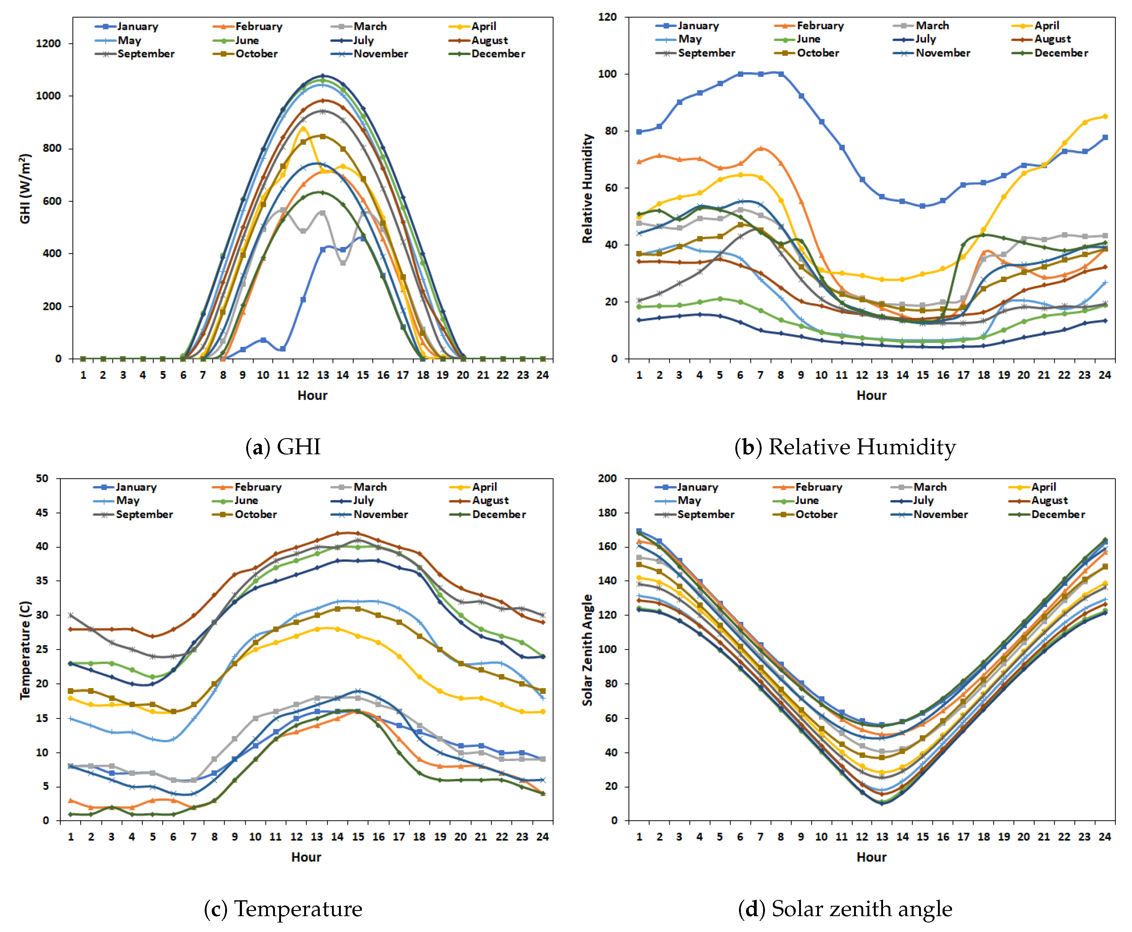
2.2. Data Description

Real-world data sets containing solar irradiance, weather, and cloud cover data are collected. Data sets range from 1 January 2004 to 31 December 2014, yielding 96,360 total observations. Hourly solar irradiance and weather data are obtained from the National Renewable Energy Laboratory’s National Solar Radiation Database for Phoenix International Airport in Phoenix, Arizona. GHI and weather variables, including solar zenith angle, relative humidity, and air temperature, from 2004 to 2014 are chosen for our experiments. These particular variables were chosen based on Pearson correlation coefficients between GHI and each of the variables, which indicates a strong linear relationship between the two variables. The Pearson correlation coefficients are $-0.87$, $-0.51$, and $0.57$ for the solar zenith angle, relative humidity, and air temperature, respectively. Figure 2 shows examples of hourly input data using the first day of each month in 2004. The time at which solar irradiance occurs at sunrise and sunset as well as the amount of solar irradiance around noon varies throughout the year. Additionally, on days where cloud cover is present, the GHI curve features sudden drops in solar irradiance through the day. For the cloud cover data set, the National Oceanic and Atmospheric Administration (NOAA) hosts the International Satellite Cloud Climatology Project (ISCCP) that provides global cloud information at high resolutions. We utilize the ISCCP HXG files which contain data in three-hour intervals at 0.1 equal angles of latitude and longitude. Within these files, cloud cover data is represented in binary with 0 and 1 indicating no cloud and cloud cover, respectively. We calculate a ratio of pixels containing cloud cover to total pixels in order to determine the surrounding cloud activity of a given location. For our experiments, we used an area of three pixels squared with the location of interest in the middle. The solar irradiance, weather, and cloud cover data are then aggregated by repeating the cloud cover ratios three times per interval to match the hourly data set. Before training the networks, the data set containing solar irradiance, weather, and cloud cover data is normalized using Min-Max normalization, reducing the range of data between zero and one.

2.3. Experimental Evaluation

In order to fully evaluate our proposed GRU network, we perform a set of three experiments. For our first experiment, we evaluate the univariate case of GRU comprising only of historical solar irradiance (i.e., GHI) from the Phoenix International Airport. Our model uses the past 48 time steps, or GHI from the last 48 h, to forecast solar irradiance at the next time step. We tested the model for 24, 48, and 72 h (one to three previous days) and found that using 48 time steps resulted in the best performance for LSTM and GRU forecasting models. Our second experiment extends the first by adding sequences of hourly solar zenith angle, relative humidity, and air temperature to build a multivariate case of GRU. Lastly, our third experiment adds the corresponding ratio of cloud cover to the multivariate model from the second experiment for a total of four exogenous variables. In both multivariate experiments, the last 48 h of data for each variable are used in training to predict solar irradiance and exogenous variables for the next hour. In order to measure model performance, we only consider the predictions for GHI.

For each experiment, the data is split into 80 percent training, 10 percent validation, and 10 percent testing in order to validate and compare model performance. The training, validation, and testing data sets are in sequence and mutually exclusive. Both GRU and LSTM are implemented using the TensorFlow and Keras libraries in Python. In order to evaluate model performance, we calculate the Mean Absolute Percentage Error (MAPE) and Root Mean Squared Error (RMSE). For a series of predicted values, the MAPE computes the average percentage error between actual and predicted values. Meanwhile, RMSE measures the standard deviation of the forecast error between actual and predicted values. MAPE and RMSE are calculated using the following formulas:

$$\begin{array}{cc}\hfill MAPE& =\frac{100}{N}\sum _{i=1}^N\frac{|A-P|}{\left|A\right|}\hfill \end{array}$$

(5)

$$\begin{array}{cc}\hfill RMSE& =\sum _{i=1}^N\sqrt{\frac{{(A-P)}^2}{N}}\hfill \end{array}$$

(6)

where A and P indicate the actual and predicted values, respectively, and N is the total number of predictions. In all experiments, the MAPE and RMSE are calculated for daylight hours only.

3. Results and Discussion

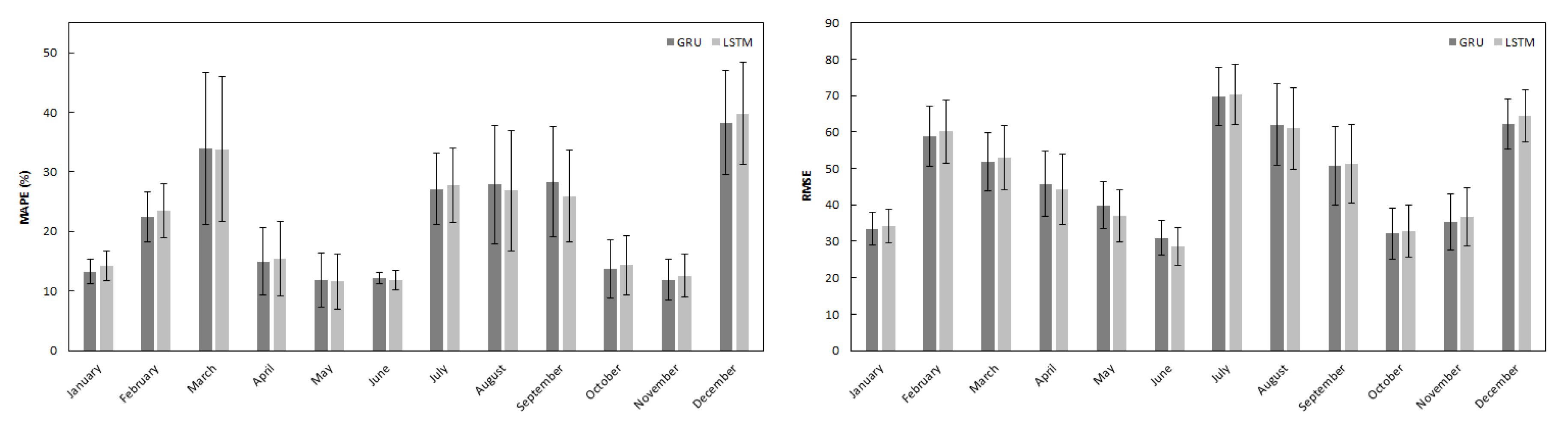
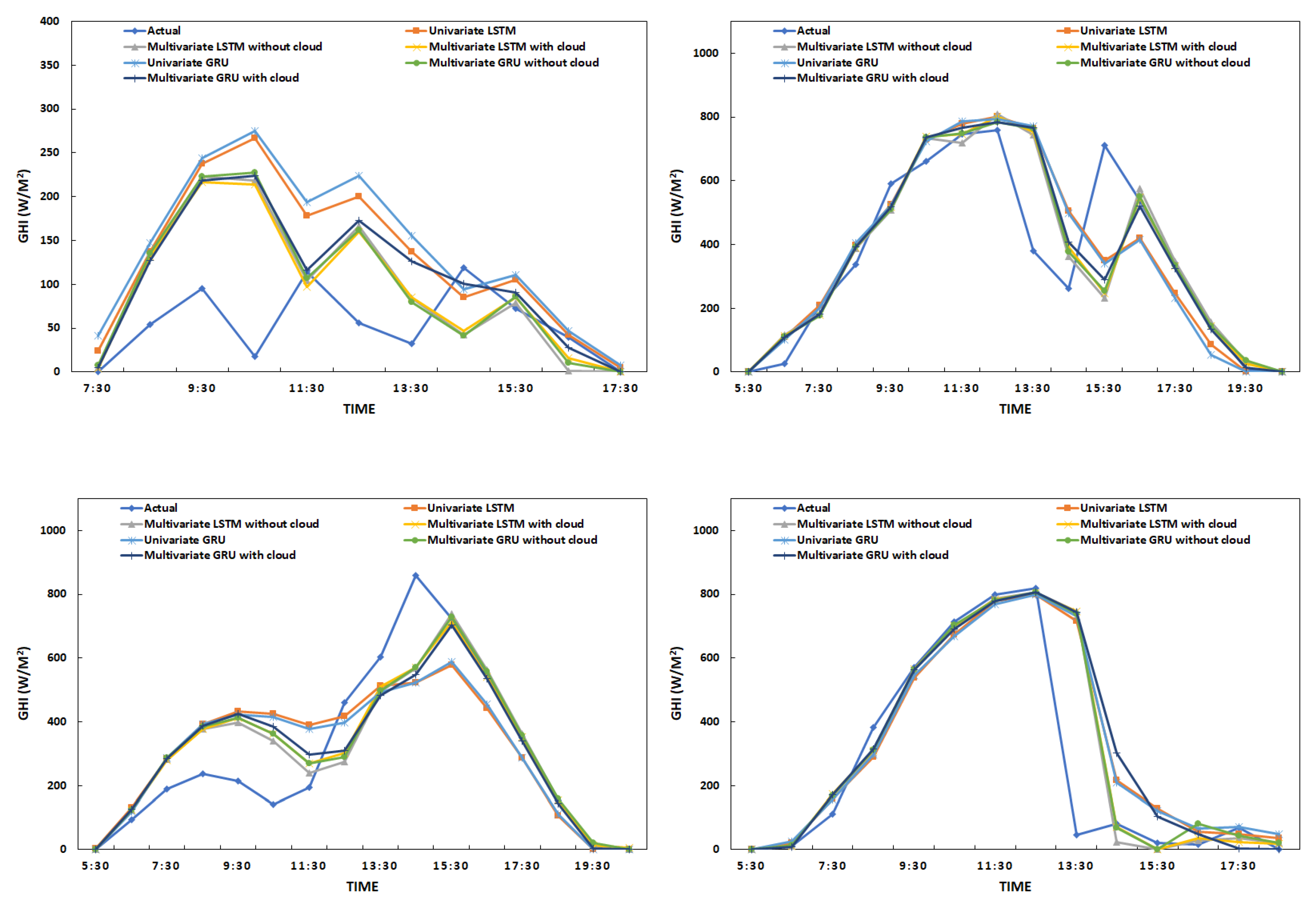
3.1. Experimental Results

Table 1. Comparison of forecast errors at one time step across one year of hourly testing data.

Model	Univariate		Multivariate without Cloud Cover		Multivariate with Cloud Cover
	MAPE	RMSE	MAPE	RMSE	MAPE	RMSE
LSTM	29.13%	67.17	25.37%	66.57	23.79%	66.75
GRU	30.29%	68.27	28.99%	67.29	25.67%	67.97

summarizes the results for hour-ahead forecasting from three experiments for LSTM and GRU: univariate models, multivariate models without cloud cover, and multivariate with cloud cover. We observe that for both LSTM and GRU, multivariate models outperform univariate models. In the case of multivariate LSTM, the improvement was 18.33% and in the case of Multivariate GRU the improvement was 15.25%. We observe that Multivariate LSTM with cloud cover has slightly better performance compared with Multivariate GRU. We further study the performance of both LSTM and GRU with multiple step ahead forecasts from 1-step ahead to 10-steps ahead forecast. We observe in Figure 3 that both GRU and LSTM based multivariate models outperform univariate models until 7 time steps ahead with no significant different between them.

Figure 4 shows the average MAPE and RMSE along with standard error bars for each month of the testing set using multivariate GRU and LSTM with cloud cover. Across all months, the average MAPE and RMSE values were very close between multivariate GRU and LSTM models. In six out of 12 months (i.e., January, April, May, June, October, and November), the MAPE values for multivariate GRU and LSTM were below 20 percent. Similarly, RMSE values below 40 occurred in five out of 12 months (i.e., January, May, June, October, and November). In both MAPE and RMSE, March, July, August, September, and December produced the highest amounts of error throughout the year. Additionally, the standard error bars are wider during these months, indicating high variation in accuracy in that time period. Figure 5 shows the actual solar irradiance and forecasting results for each of the three experiments for GRU and LSTM on four different days throughout the testing year. On these given days, cloud cover was present throughout the day and the amount of solar irradiance during daylight hours was not consistent. In all cases, the multivariate models predicted solar irradiance similarly to one another and closer to the actual values than the univariate models. The highest amounts of error occurred when the model overestimated the solar irradiance or after a sudden change in solar irradiance. On days where solar irradiance is inconsistent in the morning hours, all models overestimated the amount of solar irradiance compared to the actual values; this may be due to the fact that the models learned that solar irradiance increases consistently in the morning hours. After a sudden decrease in solar irradiance, the models react to the sudden change in the following time step, rather than accurately predicting the sudden change. Similarly, the models react to a sudden increase in solar irradiance in the time step directly after. This often led to a high amount of error if the actual solar irradiance increased after the decrease. Because of the reactivity of the models, overall error is higher on days where solar irradiance is inconsistent and stochastic. It would be helpful to seek higher resolution data for solar irradiance, weather variables, and cloud cover time series in order to combat the problems with overestimation and reacting to sudden changes in solar irradiance [25].

Despite their architectural differences, LSTM and GRU have been shown to perform similarly to one another, indicating that the superior model highly depends on the task [24]. In this case, we believe that multivariate GRU and multivariate LSTM perform similarly in terms of model accuracy. It is evident that the addition of exogenous weather variables increases solar irradiance forecasting accuracy overall; however, with the addition of weather variables, there is also an increase in the training and prediction time.

Table 2. Comparison of training and prediction time.

Experiment	Training (h)	Prediction (s)
Univariate GRU	0.65	1.55
Univariate LSTM	0.7	1.39
Multivariate GRU without cloud	2.4	8.14
Multivariate LSTM without cloud	2.66	9.23
Multivariate GRU with cloud	2.9	11.02
Multivariate LSTM with cloud	3.27	11.84

describes the training and prediction times for all experiments. Multivariate GRU and LSTM with cloud cover took approximately 4 and 6.5 times longer to train and predict than their univariate counterparts, respectively. In all cases, however, the GRU models performed faster than the LSTM models. The total number of trainable parameters for GRU are quite less compared with LSTM, hence GRU has less parameters to train in comparison to the LSTM model. The biggest difference in training time between GRU and LSTM can be seen as more variables are added to the models. Higher amounts of training and prediction times in the multivariate models may not be suitable for real-time solar irradiance forecasting, as it may take too long to update short-term forecasts based on the most recent information.

3.2. Discussion

Irradiance forecasting is a very important component for grid operators to manage the variability and uncertainty associated with solar power. Cloud cover is the most critical variable for solar energy power generation, but is also characterized by high degree of uncertainty and variability. Ground-based remote sensing equipment is needed for obtaining high resolution cloud cover data. In this paper, we studied the application of multivariate GRU for irradiance forecasting. We compared the multivariate GRU with univariate and multivariate LSTM with and without cloud cover data. We used cloud cover data obtained from satellite observations (which has much coarser resolution compared to ground-based remote sensing equipment).

We observe that existing forecasting models perform well during non-cloudy days compared to cloudy days due to a high degree of variability in cloud cover. In the proposed multivariate GRU, we used historical solar irradiance, solar zenith angle, air temperature, relative humidity, and cloud cover to predict hourly solar irradiance. Multivariate models with and without the addition of cloud cover outperformed univariate GRU and LSTM. Additionally, LSTM outperformed GRU in both univariate and multivariate experiments. We compared our forecasting results to the Phoenix results from Reikard [13] as shown in

Table 3. Comparison of forecast errors from Reikard [13].

Model	Error (%)
Regression	29.96
Unobserved Components Models	29.92
ARIMA	23.6
Transfer function	23.52
Neural network	29.38
Hybrid	23.67

and observed that multivariate GRU and LSTM with cloud cover performed similarly to their tested statistical and machine learning models. For certain months, average model accuracy was much lower due to outliers in MAPE and RMSE. In these cases, the monthly ranges for MAPE and RMSE were larger, leading to wider standard error bars. For example, there were three particular days in March where the model predicted solar irradiance with an MAPE over 100 percent. In order to improve the number of outliers, additional research is needed to develop a model that can handle generalizing a wide variation of solar irradiance patterns on cloudy days.

4. Conclusions

In this paper, we propose the application of a relatively new and robust RNN to forecast hourly solar irradiance. We applied univariate and multivariate GRU models using historical solar irradiance, exogenous meteorological variables, and cloud cover data to forecast solar irradiance in Phoenix, Arizona. The proposed is compared with LSTM, another popular deep learning model. We further analyze the performance of models to forecast multiple time steps into future, how the models perform with cloud cover variable, and how the performance of different models vary across a given day, over the year, and days with high variability in irradiance. Our primary motivation for this work is to be able to find a model that can continuously produce real-time forecasts based on publicly available weather data. Therefore, we also study the computational performance of various models. Overall, multivariate deep learning methods perform better than univariate models. There is significant performance improvement with including cloud cover in the multivariate models. We observe from Phoenix dataset that multivariate LSTM has slightly less error compared to multivariate GRU, but multivariate GRU has less training and prediction time compared to multivariate LSTM. There is not much difference between per month MAPE and RMSE between multivariate GRU and multivariate LSTM.

In our future work, we would like to improve irradiance forecasting performance that would further help grid operators to manage uncertainty associated with solar power. This includes using better quality cloud cover data in the model, techniques to further improve the performance of the model, and finally, evaluating the utility of these models to help grid operators manage the variability of irradiance under different conditions. The proposed deep learning methods could be further improved by incorporating more detailed cloud cover related features [31] as well as higher resolution GHI data. The data used in our experiments includes hourly GHI data which is freely available from NREL [32], but many solar installations collect one-minute resolution data [33] that could be used to potentially improve the model performance. On days where there is no cloud cover, both models performed exceptionally; however, on days with cloud cover, both models fail to accurately predict future solar irradiance. Rather than having one static model to predict non-cloudy and cloudy days, we could potentially use ensemble methods or concept drift methods to reduce over-fitting on days where there is high variability in cloud cover [34]. Moreover, more research is needed in not only reducing the forecast error, but also maximizing the utility of irradiance forecasts. The use of variables, namely back-of-module temperature and DNI, could be used to predict solar power plant production. Being able to predict solar power plant production using DNI and back-of-module temperature would allow power grid operators to calculate future production directly, further reducing the margin of error.

References

1. Diagne, M.; David, M.; Lauret, P.; Boland, J.; Schmutz, N. Review of solar irradiance forecasting methods and a proposition for small-scale insular grids. Renew. Sustain. Energy Rev. 2013, 27, 65–76. [Google Scholar] [CrossRef] [Green Version]
2. Kreith, F. Principles of Sustainable Energy Systems; Mechanical and Aerospace Engineering Series; CRC Press: London, UK, 2013. [Google Scholar]
3. Law, E.W.; Prasad, A.A.; Kay, M.; Taylor, R.A. Direct normal irradiance forecasting and its application to concentrated solar thermal output forecasting—A review. Sol. Energy 2014, 108, 287–307. [Google Scholar] [CrossRef]
4. Yang, D.; Jirutitijaroen, P.; Walsh, W.M. Hourly solar irradiance time series forecasting using cloud cover index. Sol. Energy 2012, 86, 3531–3543. [Google Scholar] [CrossRef]
5. Marquez, R.; Coimbra, C.F. Intra-hour DNI forecasting based on cloud tracking image analysis. Sol. Energy 2013, 91, 327–336. [Google Scholar] [CrossRef]
6. Li, J.; Ward, J.K.; Tong, J.; Collins, L.; Platt, G. Machine learning for solar irradiance forecasting of photovoltaic system. Renew. Energy 2016, 90, 542–553. [Google Scholar] [CrossRef]
7. Qing, X.; Niu, Y. Hourly day-ahead solar irradiance prediction using weather forecasts by LSTM. Energy 2018, 148, 461–468. [Google Scholar] [CrossRef]
8. Wang, Y.; Liao, W.; Chang, Y. Gated recurrent unit network-based short-term photovoltaic forecasting. Energies 2018, 11, 2163. [Google Scholar] [CrossRef]
9. Kratochvil, J.A.; Boyson, W.E.; King, D.L. Photovoltaic Array Performance Model; Technical Report; Sandia National Laboratories: Albuquerque, NM, USA.
10. De Soto, W.; Klein, S.; Beckman, W. Improvement and validation of a model for photovoltaic array performance. Sol. Energy 2006, 80, 78–88. [Google Scholar] [CrossRef]
11. Perez, R.; Lorenz, E.; Pelland, S.; Beauharnois, M.; Van Knowe, G.; Hemker, K., Jr.; Heinemann, D.; Remund, J.; Müller, S.C.; Traunmüller, W.; et al. Comparison of numerical weather prediction solar irradiance forecasts in the US, Canada and Europe. Sol. Energy 2013, 94, 305–326. [Google Scholar] [CrossRef]
12. Mathiesen, P.; Collier, C.; Kleissl, J. A high-resolution, cloud-assimilating numerical weather prediction model for solar irradiance forecasting. Sol. Energy 2013, 92, 47–61. [Google Scholar] [CrossRef] [Green Version]
13. Reikard, G. Predicting solar radiation at high resolutions: A comparison of time series forecasts. Sol. Energy 2009, 83, 342–349. [Google Scholar] [CrossRef]
14. Dong, Z.; Yang, D.; Reindl, T.; Walsh, W.M. Short-term solar irradiance forecasting using exponential smoothing state space model. Energy 2013, 55, 1104–1113. [Google Scholar] [CrossRef]
15. Melzi, F.N.; Touati, T.; Same, A.; Oukhellou, L. Hourly solar irradiance forecasting based on machine learning models. In Proceedings of the 2016 15th IEEE International Conference on Machine Learning and Applications (ICMLA), Anaheim, CA, USA, 18–20 December 2016; pp. 441–446. [Google Scholar]
16. Heinemann, D.; Lorenz, E.; Girodo, M. Forecasting of solar radiation. In Solar Energy Resource Management for Electricity Generation from Local Level to Global Scale; Nova Science Publishers: New York, NY, USA, 2006. [Google Scholar]
17. Aguiar, L.M.; Pereira, B.; Lauret, P.; Díaz, F.; David, M. Combining solar irradiance measurements, satellite-derived data and a numerical weather prediction model to improve intra-day solar forecasting. Renew. Energy 2016, 97, 599–610. [Google Scholar] [CrossRef] [Green Version]
18. Marquez, R.; Pedro, H.T.; Coimbra, C.F. Hybrid solar forecasting method uses satellite imaging and ground telemetry as inputs to ANNs. Sol. Energy 2013, 92, 176–188. [Google Scholar] [CrossRef]
19. Cao, J.C.; Cao, S. Study of forecasting solar irradiance using neural networks with preprocessing sample data by wavelet analysis. Energy 2006, 31, 3435–3445. [Google Scholar] [CrossRef]
20. Ogliari, E.; Niccolai, A.; Leva, S.; Zich, R. Computational intelligence techniques applied to the day ahead pv output power forecast: Phann, sno and mixed. Energies 2018, 11, 1487. [Google Scholar] [CrossRef]
21. Goodfellow, I.; Bengio, Y.; Courville, A. Deep Learning; The MIT Press: Cambridge, MA, USA, 2016. [Google Scholar]
22. Graves, A.; Mohamed, A.R.; Hinton, G. Speech recognition with deep recurrent neural networks. In Proceedings of the 2013 IEEE International Conference on Acoustics, Speech and Signal Processing (Icassp), Vancouver, BC, Canada, 26–31 May 2013; pp. 6645–6649. [Google Scholar]
23. Zhao, Z.; Chen, W.; Wu, X.; Chen, P.C.; Liu, J. LSTM network: A deep learning approach for short-term traffic forecast. IET Intell. Transp. Syst. 2017, 11, 68–75. [Google Scholar] [CrossRef]
24. Chung, J.; Gulcehre, C.; Cho, K.; Bengio, Y. Empirical evaluation of gated recurrent neural networks on sequence modeling. arXiv 2014, arXiv:1412.3555. [Google Scholar]
25. Alzahrani, A.; Shamsi, P.; Dagli, C.; Ferdowsi, M. Solar irradiance forecasting using deep neural networks. Procedia Comput. Sci. 2017, 114, 304–313. [Google Scholar] [CrossRef]
26. Abdel-Nasser, M.; Mahmoud, K. Accurate photovoltaic power forecasting models using deep LSTM-RNN. Neural Comput. Appl. 2019, 31, 2727–2740. [Google Scholar] [CrossRef]
27. Husein, M.; Chung, I.Y. Day-Ahead Solar Irradiance Forecasting for Microgrids Using a Long Short-Term Memory Recurrent Neural Network: A Deep Learning Approach. Energies 2019, 12, 1856. [Google Scholar] [CrossRef]
28. Kumar, S.; Hussain, L.; Banarjee, S.; Reza, M. Energy Load Forecasting using Deep Learning Approach-LSTM and GRU in Spark Cluster. In Proceedings of the 2018 Fifth International Conference on Emerging Applications of Information Technology (EAIT), Howrah, India, 12–13 January 2018; pp. 1–4. [Google Scholar] [CrossRef]
29. Sorkun, M.C.; Paoli, C.; Incel, D. Time series forecasting on solar irradiation using deep learning. In Proceedings of the 2017 10th International Conference on Electrical and Electronics Engineering (ELECO), Bursa, Turkey, 30 November–2 December 2017; pp. 151–155. [Google Scholar]
30. Cho, K.; van Merrienboer, B.; Gulcehre, C.; Bougares, F.; Schwenk, H.; Bengio, Y. Learning phrase representations using RNN encoder-decoder for statistical machine translation. In Proceedings of the Conference on Empirical Methods in Natural Language Processing (EMNLP 2014), Doha, Qatar, 25–29 October 2014. [Google Scholar]
31. Watanabe, T.; Oishi, Y.; Nakajima, T.Y. Characterization of surface solar-irradiance variability using cloud properties based on satellite observations. Sol. Energy 2016, 140, 83–92. [Google Scholar] [CrossRef] [Green Version]
32. Sengupta, M.; Weekley, A.; Habte, A.; Lopez, A.; Molling, C. Validation of the National Solar Radiation Database (NSRDB) (2005–2012); Technical Report; NREL (National Renewable Energy Laboratory (NREL): Lakewood, CO, USA, 2015. [Google Scholar]
33. Pedro, H.T.; Larson, D.P.; Coimbra, C.F. A comprehensive dataset for the accelerated development and benchmarking of solar forecasting methods. J. Renew. Sustain. Energy 2019, 11, 036102. [Google Scholar] [CrossRef] [Green Version]
34. Wojtkiewicz, J.; Katragadda, S.; Gottumukkala, R. A Concept-Drift Based Predictive-Analytics Framework: Application for Real-Time Solar Irradiance Forecasting. In Proceedings of the 2018 IEEE International Conference on Big Data (Big Data), Seattle, WA, USA, 10–13 December 2018; pp. 5462–5464. [Google Scholar]
Figure 1. Structure of a Gated Recurrent Units (GRU) cell [24].
Energies 12 04055 g001
Figure 2. Hourly input data for the first day of each month in 2004.
Energies 12 04055 g002
Figure 3. Mean Absolute Percentage Error (MAPE) and Root Mean Squared Error (RMSE) values for each model predicted ten time steps into the future.
Energies 12 04055 g003
Figure 4. Average MAPE and RMSE values with corresponding standard error for each month using multivariate GRU and Long Short-Term Memory (LSTM) with cloud cover.
Energies 12 04055 g004
Figure 5. Comparison of actual and forecast values for both LSTM and GRU models on days with irregular solar irradiance patterns.
Energies 12 04055 g005