Abstract
The Reynolds-averaged Navier–Stokes (RANS)-based generalized actuator disc method along with the Reynolds stress model (AD/RANS_RSM) is assessed for wind turbine wake simulation. The evaluation is based on validations with four sets of experiments for four horizontal-axis wind turbines with different geometrical characteristics operating in a wide range of wind conditions. Additionally, sensitivity studies on inflow profiles (representing isotropic and anisotropic turbulence) for predicting wake effects are carried out. The focus is on the prediction of the evolution of wake flow in terms of wind velocity and turbulence intensity. Comparisons between the computational results and the measurements demonstrate that in the near and transition wake region with strong anisotropic turbulence, the AD/RANS_RSM methodology exhibits a reasonably good match with all the experimental data sets; however, in the far wake region that is characterized by isotropic turbulence, the AD/RANS_RSM predicts the wake velocity quite accurately but appears to over-estimate the wake turbulence level. While the introduction of the overall turbulence intensity is found to give an improved agreement with the experiments. The performed sensitivity study proves that the anisotropic inflow condition is recommended as the profile of choice to represent the incoming wind flow.
1. Introduction
Wind turbine wake effects are associated with a decrease in the downstream wind speed and an enhancement in the turbulence fluctuations, which further results in a reduction in the power output and a high risk of structural fatigue issues for downstream turbines. Reliable methods for the accurate modelling of wake effects are imperative, ultimately, for optimizing the layout and mitigating fatigue hazards of turbines within wind farms. As computational power continues to grow and numerical techniques are continuously refined, computational fluid dynamics (CFD) is rapidly being adopted as a key tool for wind turbine wake simulations [1,2,3,4]. In this process, accurate modellings of the turbine rotor and turbulent flow are two crucial points and ongoing challenges.
For the first key point, the approaches that exist to represent the turbine rotor are summarized as full rotor approach (direct approach) and generalized actuator approach [5]. Due to its high demand for computing resources, the full rotor method is seldom applied in engineering practice, especially for wind farm simulations. The most commonly used approach is the generalized actuator method, including actuator disc (AD), actuator line (AL), and actuator surface (AS) models. Among the three of them, the AD model, with the fundamental idea of using a permeable disc of an equivalent area to represent the turbine rotor, has been a popular tool of the renewable energy industry for wind turbine wake simulations [6,7,8,9,10]. Despite its simplicity, this AD model has proved its abilities of predicting wake effects with reasonable accuracy for isolated wind turbines [5,9,11,12,13], as far as the far wake is concerned.
Another important piece is to model the turbulent wind flow. It was realized early that Reynolds-averaged Navier–Stokes equations (RANS) in association with the AD approach (AD/RANS) are a promising concept to predict the wake flow. Turbulence models for RANS equations are numerous; for wake simulations, the most popular and widely used ones are the standard k-ε model and the shear stress transport (SST) k-ω model. However, previous works [1,8,11,14,15] consistently indicated that when combined with the AD approach, these two-equation turbulence closures failed to predict the wake behavior accurately. Réthoré [16] and Laan et al. [11] explained that the failures of these two-equation models are attributed to the limitations of the Boussinesq hypothesis. Accordingly, a series of modified turbulence models was continuously proposed to address the weakness of the Boussinesq hypothesis, and it was declared that the obtained results featured a higher accuracy than those from the standard models. However, as noted by Shives [8] and Hu et al. [3], many of these modified models are heavily dependent on the empirical correction of turbulence production or dissipation, and the general applicability of them meets a big challenge.
On the other hand, Gómez et al. [17] found out that an intense anisotropic turbulence exists in the near wake flow and indicated that rather than the isotropic turbulence models, the Reynolds stress model (RSM), accounting for the anisotropic turbulence stresses, was potentially the most performant model. Cabezón et al. [18] compared various k-ε-based turbulence models and the RSM, then illustrated that RSM estimated the wake deficit accurately in both near and far wake flow, and also gave acceptable predictions of the turbulence intensity. Additionally, Makridis et al. [9] found out that with the RSM the predicted wake deficit was in good agreement with the measurements at hub height. Furthermore, in the work of Hu et al. [3], RSM showed a good performance in predicting the turbine wake properties as compared with the wind tunnel test data. All these works proved that RSM can give a better solution than isotropic models. By contrast, Nguyen et al. [19] tested four classic turbulence models and indicated that the best agreement with experimental data was obtained with the standard k-ε model instead of the RSM. Besides, [8,20] pointed out that the complexity of RSM does not always guarantee to give the best results compared to the simpler one- or two-equation turbulence models. To sum up, on one hand, a number of studies have been performed to provide insight into the performance of the RSM, but the findings are not conclusive. On the other hand, most studies have employed a limited set of cases for validation; thus, the generalization of the findings may not be fully supported.
Therefore, in this present work, a comprehensive analysis is performed to evaluate the accuracy of the AD/RANS method with the RSM (for convenience, this is herein referred to as the AD/RANS_RSM methodology) for wind turbine wake simulations. In this process, the wide diversity of the test cases and analyzed parameters helps to scrutinize the performance of the AD/RANS_RSM methodology and support the generalization of the findings of the present study. In addition to this, it has been found that the inlet conditions affect the CFD modelling significantly [21]. However, different expressions of the inlet profile were used in previous works, such that [19,22] used isotropic inflow conditions, while [3,9,18] employed anisotropic profiles. Therefore, a sensitive analysis of the influence of distinct inflow profiles on wake predictions when using the AD/RANS_RSM method is desirable, which is going to be conducted in this study.
The paper is prepared in the following manner. Section 2 and Section 3 are dedicated to introducing the theoretical backgrounds of the AD/RANS_RSM methodology and the computational settings. A case description, sensitivity analysis of inflow conditions, and performance comparisons and discussions of the AD/RANS_RSM method are presented in Section 4. Finally, concluding remarks are made in Section 5.
2. Numerical Methodologies
2.1. Governing Equations
The incompressible steady RANS equations are used for simulating the atmospheric turbulent wind flowing through wind turbines, which can be written in Cartesian coordinate as follows:
where ρ is the air density, P is the pressure, xi is the coordinate system, ui or uj is the velocity vector (u, v, w), µ is the fluid dynamic viscosity, is the unknown Reynolds stress tensor, and is the force exerted by the disk on the fluid, which will be discussed in Section 2.3.
2.2. Reynolds Stress Model (RSM)
Previous works [1,8,11,14] stated that the intrinsic feature of the neutral atmospheric turbulence is anisotropic, and the RSM has the potential of accurately predicting the anisotropic atmospheric turbulence as well as the anisotropic wake, which is an important advantage as the eddy viscosity approach is avoided, and relies on the exact Reynolds stress transport equation. In this RSM, the turbulence closure is achieved by applying one transport equation for each individual component of the Reynolds stress tensor and additionally one equation for the dissipation rate ε, corresponding to 6 + 1 = 7 equations; this further makes the RSM the potentially higher-level and physically the most complete model. The linear pressure-strain RSM is employed in the present work, and detailed information and formula can be found in the ANSYS fluent manual [23]. Since the number of transport equations is increased, RSM requires on average 50–60% more computational time and 15–20% more CPU memory when compared to the eddy-viscosity-based models like k-ε or k-ω models.
2.3. Actuator Disc Model
The one-dimensional actuator disc (AD) [8,14] technique is proposed with the basic idea of representing the turbine rotor by a porous disk on which a thrust force fturb is evenly distributed. Without considering blade rotation effects, the AD model cannot provide a precise description of the near wake flow within 3D (D is the turbine diameter). However, it has proven its adequate capability to model the far wake flow where the swirl effect is assumed to be dissipated [1,8,19,24]. In the AD method, the turbine-induced force is incorporated into the RANS equations (see Equation (2)) as a negative source term, which is described as:
where u0,hub is the incoming wind speed at hub height, Ct is the thrust coefficient that can be obtained from the Ct—velocity curve of the turbine. From Equation (3), it can be seen that the calculation of fturb only requires the rotor diameter D, the thrust coefficient, and the incoming hub height wind speed, which are usually available for turbines.
3. Computational Settings
3.1. Computational Domain and Boundary Conditions
The computational domain is constructed according to the Architectural Institute of Japan (AIJ) guidelines [25], as illustrated in Figure 1a with its main boundary conditions, and this domain is used for all the test cases. Moreover, the corresponding computational settings are summarized in Table 1. For the ground layer, the grids are refined to gain y+ values between 30 and 300 (it is in the accepted range for the wall function approach used in the computations), getting nearly 50 nodes below hub height for all the test cases. In order to resolve the strong gradients around the turbine rotor, a high concentration of grid points is distributed in the vicinity of the rotor, with the generated mesh shown in Figure 1b. Finally, the total number of grid points used for the computations is around 3.8 million. Similar grid resolutions have been employed in previous studies [1,7,14,15] that used the actuator-type models, and they have been proven sufficient to capture the wake characteristics behind a single turbine.
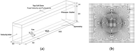
Figure 1.
(a) Computational domain with its main boundary conditions and (b) computational mesh in the vicinity of the turbine rotor.

Table 1.
Summary of computational set-up in the computational fluid dynamics (CFD) models.
3.2. Isotropic and Anisotropic Inflow Conditions
For every CFD analysis, accurate inflow conditions are paramount to the fidelity of the outcome. It was observed [21,26] that on one hand, wind turbine wake problems are very sensitive to inflow conditions; on the other hand, different expressions of the inlet profile exist in the literature when using the RSM. Therefore, a sensitive analysis of the influence of incoming wind profiles on the downstream wake flow was performed. The adopted inflow profiles (which are classified into isotropic and anisotropic inflow profiles) are listed in Table 2, in which the velocity profile u(z) is characterized by the power law, which is widely used in wind engineering applications due to its simplicity and practicality. As regarding the turbulence quantities k, ε, and ω, they are fundamental for the RSM but difficult to be estimated directly; instead, it is an effective way to relate them to easily obtained parameters such as the wind speed u and turbulence intensity TI. Therefore, the mostly used relation typically resorted to is to derive k using Equation (6). Accordingly, the values of ε and ω are estimated with the assumption of a local equilibrium, as given by Equations (7) and (8).
Table 2.
Summary of adopted turbulence profiles required at the inlet and outlet boundaries.
It should be noted that the RSM in ANSYS FLUENT requires boundary conditions for each of the Reynolds stresses . If their values are not specified explicitly at the inlet, then the turbulence is assumed to be isotropic (as described by Equation (9)); if the anisotropic property of the atmospheric boundary layer (ABL) turbulence is considered, the normal and shear Reynolds stress profiles have the form as given in Equation (10) [9,27]. Note that for these two types of inflow conditions, the profiles of u, TI, ε, and ω are identical, in which the variables uhub and TIhub are defined at a reference height, i.e., hub height, and α is the power-law exponent that can be determined according to the surface roughness categorization [28] upwind of the site. Note that the value of α is set to be 0.15 for all the following test cases. On the other hand, the difference between two sets of profiles reflects in three aspects: (1) calculation of the turbulence kinetic energy k; (2) the expression of each Reynolds stress; (3) the value of the RSM constant Cμ [2].
4. Results and Discussion
The wind turbine wake area is typically divided into two parts [17]: near wake and far wake. The former is the region that falls in the range of 2D (D is the rotor diameter of the turbine) to 5D downstream from the rotor disc, after which there is a small transition zone leading to the far wake region, where the wake is completely developed. Correct prediction of the wake recovery in terms of wind velocity and turbulence intensity is of paramount importance for the accurate estimation of power production and fatigue impact on downstream facilities. Thus, in the following part, special emphasis will be placed on quantifying the predicted magnitude and spatial distribution of the wake velocity and the enhancement of the turbulence level in the wake flow.
4.1. Case 1: Wind Tunnel Experiment (WiRE Rotor)
In 2009, wind tunnel experiments [29] were carried out in the St. Anthony Falls Laboratory atmospheric boundary-layer wind tunnel. The studied object was a miniature wind turbine with a three-blade GWS/EP-6030 rotor attached to a small DC generator, and it had a rotor diameter D = 0.15 m and a hub height zhub = 0.125 m. High-resolution spatial and temporal measurements were collected using a three-wire anemometer, and key turbulence quantities at different downstream locations (x/D = 3, 5, 7, 10, 14, 20) at zero span ((x, z)|y=0) were obtained and analyzed. The inflow wind speed and turbulence intensity at the hub height were estimated to be 2.2 m/s and 6.8%, respectively. Then based on the calculation of axial force, the thrust coefficient Ct was estimated as 0.56 [30].
Figure 2 displays vertical profiles of the flow statistics (including the stream-wise velocity and the stream-wise turbulence intensity) obtained from AD/RANS_RSM simulations under two inflow conditions. Moreover, results from both the wind tunnel experiment and simulations of Wu et al. [4] were gathered for cross validation. From Figure 2a, it can be seen that the AD/RANS_RSM presents acceptable prediction of the wake velocity in the near wake and transition regions (x < 5D), while the velocity is slightly over-predicted in the center of the wake; this over-prediction was also reported in [4] using the AD/LES (large-eddy simulation) method, as the blue lines show in this figure. This discrepancy can be attributed to the limitations of the assumptions made in the one-dimensional AD model [7,30]: (1) the effect of turbine-induced rotation is ignored; (2) the effect of turbine hub and nacelle are ignored; and (3) uniform force instead of radial variant force distributed over the AD surface. When it comes to the far-wake region (x > 5D), the predictions of AD/RANS_RSM improved and providing an excellent agreement with the wind tunnel data throughout the entire far wake. We can also note that the predictions obtained under the two inflow conditions are quite similar to each other, with the simulated wake velocity under the anisotropic condition closer to the measurements (both in terms of the deficit amplitude and the shape) than that under the isotropic condition.
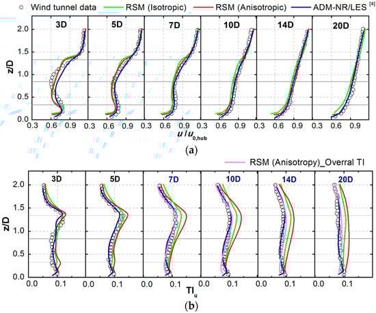
Figure 2.
Comparison of simulated and measured vertical profiles of (a) normalized stream-wise velocity and (b) stream-wise turbulence intensity (TIu). The panels from left to right indicate the flow quantity profiles at different downstream distances behind the turbine. The horizontal gray lines represent top tip, hub height, and bottom tip heights.
Focusing on the stream-wise turbulence intensity (TIu) provided by the AD/RANS_RSM method, it is possible to see that at the near wake locations of 3D and 5D, the simulations match very well the experimental observations; however, the agreement was not good for the locations further downstream (x > 5D) where an obvious over-estimation can be observed. This varied performance existing in the near and far wake regions was also observed in previous works [3,8,18] and might be due to the following reasons: the turbulence characteristic in the near wake region is strongly anisotropic [17,31,32], and the RSM is superior for situations in which the mean flow dynamics are dominated by the anisotropy of turbulence, thus showing a good ability to simulate the profile of TIu; however, when it comes to the subsequent downstream far wake area, the turbulence anisotropy has a tendency to reduce toward isotropic turbulence [2,17], and in this case, the RSM fails to reproduce the isotropic characteristics of the far wake flow and seriously over-predicts the TIu profile in this region.
Afterwards, based on the calculated results from the AD/RANS_RSM method under the anisotropic inflow condition, the overall turbulence intensity which is defined in Equation (11) is introduced and included in Figure 2b (illustrated with the magenta color lines).
where , , and are the x/y/z-component of the turbulent fluctuations, respectively. Figure 2b clearly shows that the profile of overall TI presents an obvious improved agreement with the measured data in the far wake region. This demonstrates that the RSM over-predicts the value of the stream-wise turbulence intensity TIu, while the averaged TI in all the three directions can be a good representation of the isotropic turbulence in the far wake region.
In order to conduct a more rigorous validation of the AD/RANS_RSM method with the anisotropic inflow condition, two parameters, average relative error ( = and maximum relative error ( = ), are introduced for quantitative comparison, where illustrates the value from the experiment, is the value from the AD/RANS simulation, and N is the number of the measured point. The obtained errors are presented in Table 3. It can be seen that the AD/RANS_RSM method performs well to predict the wake velocity with Eave around 3% and Emax under 13.2% throughout all wake positions, whereas these two errors reduce to about 2% and below 6%, respectively, in the far wake region. In regard to the turbulence level, an average deviation of around 12% is found at the near wake positions. This large discrepancy is believed to be caused by the fact that the fluid motion due to the blade rotation effect is ignored in the AD model, which does not fit the measured reality. When it comes to the far wake region, with the post-processed overall TI, the AD/RANS_RSM method reduces Eave to around 6% and Emax to around 13%, and an obvious improvement can be observed.
Table 3.
The simulation’s relative error at several downstream positions behind the turbine. Note that numerical results are obtained by the AD/RANS_RSM method with the anisotropic inflow condition, and the overall TI is introduced for far wake positions (as illustrated in Figure 2b).
4.2. Case 2: Field Measurements (Sexbierum Wind Farm)
In 1992, an extensive series of measurements was carried out at an onshore wind farm with homogenous flat terrain mainly covered by grass [33]. The Sexbierum wind farm was composed of 18 HOLEC wind turbines, each with a rated power of 310 kW, rotor diameter of 30 m, and hub height of 35 m. Measurements were performed to collect data on the wind speed, turbulence level and shear stress in the wake of a single wind turbine at distances of 2.5D, 5.5D, and 8.0D, through three masts that contain three-component anemometers at hub height. The measured data were analyzed on the basis of 3-min averaged samples. The incident wind speed and turbulence intensity at hub height were estimated to be 8.4 m/s and 11%, respectively. Under these conditions, the thrust coefficient of the turbine was supposed to be 0.75.
A comparison was drawn at the central y-z plane of the wake at distances of 2.5D, 5.5D, and 8.0D downstream of the turbine. As can be noticed in Figure 3, the simulated velocities match well with the measurements at x = 2.5, 5.5D and even better than those of the AL/LES method given in [6]; moreover, there is little difference between the results obtained under two inflow conditions. However, the agreement was not as good as at the location of 8.0D further downstream. More specifically, with the anisotropic inflow condition, the wake width is well predicted but the maximum wake deficit at the wake center is under-predicted by approximately 18%; when using the isotropic inflow condition, the wake width is narrowed, but the maximum wake deficit is almost identical to the measurements. This might raise a question: which inflow profile is superior in this case?
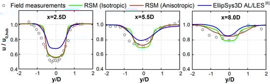
Figure 3.
Horizontal distributions of normalized wake velocity at hub height at downstream distances of 2.5D, 5.5D, and 8.0D. Comparison between predictions obtained from the AD/RANS_RSM under isotropic and anisotropic turbulence inflow conditions, and field measurements (experimental data obtained from Cleijne [33]). Besides, in order to avoid the uncertainty in measurements and assess the performance of the AD/RANS method fairly, numerical results [6] obtained from the AL/LES computations using Technical University of Denmark (DTU’s) CFD solver EllipSys3D are also included.
In [6,34], it is pointed out that the atmosphere was very likely to be stable during the measured period, and low turbulent mixing occurring in the stable atmosphere would further lead to a much slower velocity recovery. This explains the over-estimation of the predictions with the anisotropic inflow profiles as well as the LES results in [6], since a neural atmospheric stability is assumed in these works. Overall, it comes to a preliminary conclusion that the anisotropic treatment of the inflow outperforms the isotropic inflow not only in the near wake but also in the far wake, which gives a more accurate prediction of the wake expansion downstream of the turbine. A closer look at Figure 3 shows that the measured wake shape is obviously not symmetrical in contrast to the symmetrical shape of the numerical results, due to the fact that the full-scale measurements were influenced by surrounding turbines or some obstacles while these influencing factors cannot be considered in the CFD simulations, and as a result, the simulated wake is more symmetrical in the lateral direction.
In order to investigate the non-isotropic characteristics of turbulence in wind turbine wakes, Figure 4 shows the evolution of turbulence intensity in three flow directions at different downstream distances. From the measured data, a clear double-peak profile can be observed in the near wake position (x = 2.5D), with these peaks positioned near the turbine edge, which is mainly due to the presence of helicoidal vortices (derived from tip vortices) and the induced strong shear in that region. It is furthermore seen that a strong anisotropy is shown at the edge of the wake, which is characterized by the phenomenon that the stream-wise turbulence is dramatically amplified by the tip–air interaction, resulting in a much higher value than the lateral and vertical turbulence with TIu > TIv > TIw. As the wake progresses downstream, the flow becomes more isotropic. To be more specific, at the position of x = 5.5D, it is seen that TIu has peaks in the shear layer, whereas TIv and TIw have an almost flat profile in the core of the wake. In the subsequent far wake position of 8.0D, it is noticed that the double peak effect is almost negligible, and the turbulence becomes more uniform because of the wake mixing process. Moreover, the measurements also illustrate that the turbulence is more isotropic at the wake center, with all components having approximately the same value throughout the whole wake region.
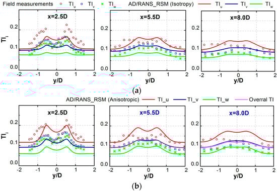
Figure 4.
Comparison of turbulence intensity in three flow directions at different downstream distances. (a) Results of the AD/RANS_RSM method under the isotropic inflow condition; (b) results of the AD/RANS_RSM method under the anisotropic inflow condition.
In Figure 4, by comparing the simulations (obtained under two inflow conditions) with the field measurements, it can be observed that the differences between two sets of predictions (as shown in Figure 4a,b) are pronounced. More specifically, at the near wake position of x = 2.5D, the AD/RANS_RSM method with the anisotropic profile reproduces satisfactorily the measured distributions of TIu, including the double-peak effect observed around at both sides of the wake axis, whereas the isotropic condition leads to an under-estimation of TI in both shear layers. Furthermore, both models consistently under-estimate the values of TIw to a great extent at x = 2.5D. This discrepancy is mainly due to the difference between the simulated and measured wind conditions. To be specific, the initial values of the Reynolds stress components are specified as and (deduced from Equation (10)), and a wide disparity exists in the three components, whereas the measured components TIv and TIw are almost equal to each other and approximately equal to 75% of TIu. This implies that the measured anisotropy is smaller than that of the numerically specified one for the incoming wind flow.
It is furthermore seen that the estimation of TIu fails at the far wake sections (such as 5.5D and 8.0D). An obvious over-estimation is observed at the center of the wake with a higher shear stress zone, even though AD/RANS_RSM shows an acceptable representation of the turbulence intensities TIv and TIw, particularly at the central axis. Furthermore, like in the first case, through post-processing of the data obtained under the anisotropic inflow, the profile of overall TI is also presented in Figure 4b. The value of overall TI is found to be reasonably close to that of TIv, due to its initial value (as deduced from Equation (10)) being almost equal to that of TIv. It can be speculated that if the initial values of three components are specified according to the measured data instead of the surface boundary layer (SBL) theory [27], the agreement between simulations and the measurements would be greatly improved.
4.3. Case 3: Field Measurements (Nibe Wind farm)
In the 1980s, field measurements of a single wind turbine (which features a hub height and a rotor diameter of 45 and 40 m, respectively) at the Nibe site were conducted by Taylor [35]. Four meteorological masts were placed at different downstream positions (2.5D, 4.0D, 6.0D, and 7.5D); due to the influence of the standstill turbine—Nibe A. The measurements at x = 4.0D will not be discussed in the following analysis. The incoming wind conditions at hub height were wind speed U0 = 8.55 m/s (this speed was not directly measured but estimated from the measured power and the power curve of the Nibe B wind turbine) and stream-wise turbulence intensity TIu = 10%. Under these conditions, the thrust coefficient was estimated to be Ct = 0.82.
Figure 5 describes the lateral evolutions of the normalized wind speed and the turbulence intensity obtained with the AD/RANS_RSM method under two different inflow profiles compared with the experimental data at each mast. By looking at the velocity profiles, at the near wake position of x = 2.5D, the wake deficit is well predicted at the wake center, but the wake is narrowed in the lateral direction by the AD/RANS_RSM method as compared with the field measurements as well as the results from [9]. When it comes to the far wake positions, it can be remarked that the RSM with the anisotropic inflow predicts much better the distribution and magnitude of the wake deficit than that under the isotropic inflow profile. Again, it proves the accuracy of the AD/RANS_RSM methodology and meanwhile shows the superiority of the anisotropic inflow conditions to some extent.
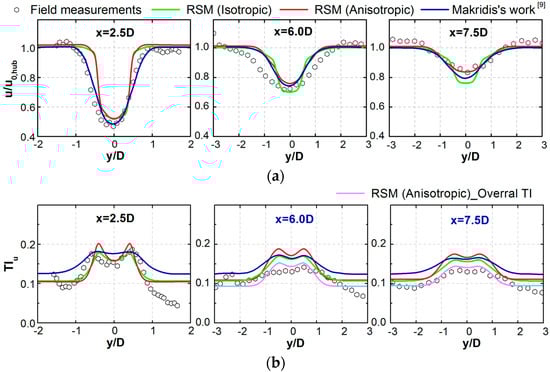
Figure 5.
Comparison between the measured and simulated lateral profiles of (a) normalized wake velocity and (b) stream-wise turbulence intensity at the downstream positions of 2.5D, 6.0D, and 7.5D.
The turbulence results presented in Figure 5b show that the AD/RANS_RSM accurately predicts the dual-peak pattern, which resulted from the rotor tip vortices and high shear production caused by the strong velocity gradient at the wake boundary. When it comes to the far wake region (x = 6.0D and x = 7.5D), the turbulence spreads more in the lateral direction, and the wake turbulence decays and becomes more uniform; at these positions, the wake turbulences are over-predicted by approximately 22% and 29% near the wake centerline with the isotropic and anisotropic inflow conditions, respectively. Similar to above two cases, introducing the parameter-overall TI improves the turbulence prediction in the far wake region, especially at the 7.5D section where it matches almost perfectly all the data points. As regards the results from [9], it can be seen that the used modified AD/RANS_RSM gives acceptable values of the wake velocity but over-estimates the turbulence level to a great extent at all the downstream locations.
4.4. Case 4: AD/LES Simulation (Vestas 2MW Wind Turbine)
In the year of 2015, a large eddy simulation combined with the rotational actuator disk model was employed to investigate wind turbine wake effects [13]. In this work, a Vestas V80-2MW wind turbine (which features a rotor diameter and hub height of 80 and 70 m, respectively) was chosen as the study object. A detailed analysis was focused on the spatial distributions of the mean velocity deficit as well as the turbulence statistics in the wake region. The incident wind velocity and turbulence intensity at hub height were set to be 8 m/s and 0.078, respectively; then according to the operational records of the turbine, its thrust coefficient Ct was determined to be 0.8.
Comparisons of the predicted vertical profiles of the wake velocity and overall TI at chosen downstream locations (x/D = 4, 8, 12, 16, and 20) are shown in Figure 6. From Figure 6a, it is clearly seen that the AD/RANS_RSM method exhibits an almost excellent match with the measured data at all the downstream positions. It can also be depicted that there is no significant difference between the results obtained under isotropic and anisotropic inflow approaches, except at the position of 4D where the isotropic profile under-estimates the wake deficit, relatively to the LES simulations, at the wake center and over-estimates it near the edge of the wake; a slight over-estimation of the wake deficit along the vertical wake affected region can also be observed at the position of 8D.
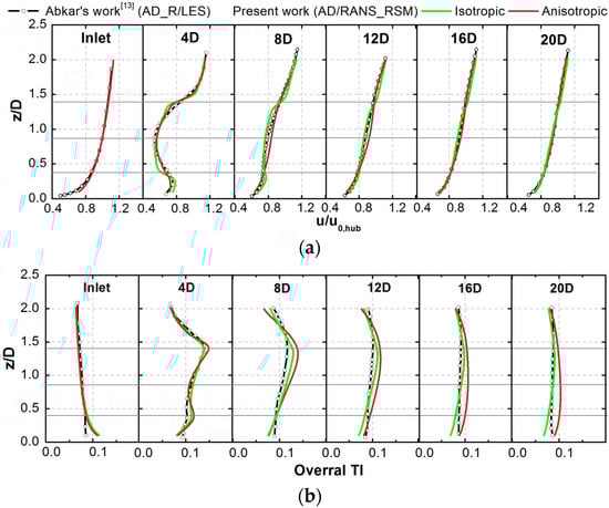
Figure 6.
Vertical profiles of (a) wake velocity and (b) overall TI for the downstream locations of 4D, 8D, 12D, 16D, and 20D. The horizontal gray lines represent top tip, hub height, and bottom tip heights.
In many wind engineering applications, in order to calculate the turbulence-induced unsteady loads, it is crucial to have reliable values of the turbulence fluctuations in all three spatial directions, especially the component in the main wind direction (which is the most significant one to estimate loads in the downstream turbines). Note that the most important parameter (stream-wise turbulence intensity) was analyzed and discussed in the above test cases, while in this case, following the work of Abkar et al. [13], the averaged overall turbulence intensity was investigated. Figure 6b shows that there are acceptable agreements with the AD_R/LES simulations in the near wake region up to 4D, while an obvious overestimation of the overall TI can be observed at all far wake locations, among which the anisotropic inflow approach performs worse than the isotropic case, with an over-estimation of up to 17% at far wake sections. This over-estimation of the overall turbulence level by the RSM has been also reported in previous works [3,8,9].
It is furthermore seen that, just like the wind tunnel case, the TI is clearly vertically non-asymmetric distributed. To be specific, the simulations show a strong enhancement of the turbulence intensity at the level of the top tip of the turbine, and higher values of overall TI can be observed. This can be attributed to the high gradient of the stream-wise velocity caused by the wind shear in addition to the strong shear caused by the wake along the vertical direction. By contrast, at the bottom-tip of the turbine, the turbulence intensity is almost equal to or less than that of the inflow due to the negative or small velocity gradient.
5. Conclusions
A comprehensive assessment of the AD/RANS_RSM methodology for horizontal-axis wind turbine wake simulations was presented in this work. The performance analysis was based on validation against four sets of experimental data using turbines with dissimilar geometrical (with diameters ranging from 10 cm (wind tunnel scale) to about 100 m (utility scale)) and operational conditions. Such a wide diversity of the test cases further supports the generality of the findings. The focus is put on the evolution of wake flow in terms of the wind velocity and turbulence intensity. In addition, a sensitivity analysis of the influence of inflow conditions on the predicted wake characteristics was carried out, with the main purpose to establish recommendation for the proper use of the RSM in wake prediction.
Comparisons of the present simulations with the reference data that was obtained from wind tunnel experiments, field measurements, and high-resolution LES simulations illustrated that the AD/RANS_RSM methodology has a quite good correspondence with all the reference data set in terms of the wake speed. Besides, this method was found to be capable of exhibiting reasonable agreement with the measured turbulence level in the near wake region but tends to over-estimate it in the far wake area. This might be explained by the finding that the near wake flow is characterized by the intense anisotropic turbulence. The RSM is only superior for accounting for the anisotropy in turbulent flow; therefore, it presented a good to excellent agreement with the reference data. By contrast, the turbulence has a tendency to become more isotropic in the subsequent far wake region because of turbulent mixing with the outside undisturbed flow, and in this case, the RSM fails to reproduce the isotropic characteristics of flow, which therefore over-predicts the turbulence level to some extent.
Through the performed sensitivity study, a significant influence of two inflow profiles (which are classified into isotropic and anisotropic profiles) on the wake behavior were observed. Particularly, the simulated wake velocities under anisotropic condition are in better agreement with the reference data (both in terms of the amplitude and the shape) than those under the isotropic condition. With the isotropic inflow profiles, the AD/RANS method appears to under-predict the wake recovery and narrow the wake width, which results in an unrealistic prediction of the wake development. As regarding the turbulence intensity, for the reason mentioned above, the results obtained with both inflow conditions consistently over-predict the wake turbulence level in the far wake area, while the results from the anisotropic condition seem to deviate from the reference data with a maximum discrepancy of up to 30%. However, the introduction of the averaged overall turbulence intensity is found to give an improved agreement with the experiments in all the test cases. In summary, to obtain reliable wake effect predictions, the anisotropic inflow condition is recommended as the profile of choice to represent the incoming wind flow.
Author Contributions
Methodology, L.T. and N.Z.; Supervision, N.Z. and T.W.; Validation, L.T., Y.S. and W.S.; Visualization, Y.S.; Writing—original draft, L.T.; Writing—review & editing, W.S. and T.W.
Funding
This research was funded by National Natural Science Foundation of China with the grand number No. 11802122.
Acknowledgments
The authors would like to acknowledge the financial support from National Natural Science Foundation of China (No. 11802122) and China Postdoctoral Science Foundation (2018M642242).
Conflicts of Interest
The authors declare no conflict of interest.
References
- Bouras, I.; Ma, L.; Ingham, D.; Pourkashanian, M. An improved k–ω turbulence model for the simulations of the wind turbine wakes in a neutral atmospheric boundary layer flow. J. Wind Eng. Ind. Aerodyn. 2018, 179, 358–368. [Google Scholar] [CrossRef]
- Antonini, E.G.A.; Romero, D.A.; Amon, C.H. Improving cfd wind farm simulations incorporating wind direction uncertainty. Renew. Energy 2019, 133, 1011–1023. [Google Scholar] [CrossRef]
- Hu, J.; Yang, Q.; Zhang, J. Study on the wake of a miniature wind turbine using the reynolds stress model. Energies 2016, 9, 784. [Google Scholar] [CrossRef]
- Wu, Y.-T.; Porté-Agel, F. Large-eddy simulation of wind-turbine wakes: Evaluation of turbine parametrisations. Bound. Layer Meteorol. 2011, 138, 345–366. [Google Scholar] [CrossRef]
- AbdelSalam, A.M.; Ramalingam, V. Wake prediction of horizontal-axis wind turbine using full-rotor modeling. J. Wind Eng. Ind. Aerodyn. 2014, 124, 7–19. [Google Scholar] [CrossRef]
- Göçmen, T.; Laan, P.V.D.; Réthoré, P.-E.; Diaz, A.P.; Larsen, G.C.; Ott, S. Wind turbine wake models developed at the technical university of denmark: A review. Renew. Sustain. Energy Rev. 2016, 60, 752–769. [Google Scholar] [CrossRef]
- Behrouzifar, A.; Darbandi, M. An improved actuator disc model for the numerical prediction of the far-wake region of a horizontal axis wind turbine and its performance. Energy Convers. Manag. 2019, 185, 482–495. [Google Scholar] [CrossRef]
- Shives, M.; Crawford, C. Adapted two-equation turbulence closures for actuator disk rans simulations of wind & tidal turbine wakes. Renew. Energy 2016, 92, 273–292. [Google Scholar]
- Makridis, A.; Chick, J. Validation of a cfd model of wind turbine wakes with terrain effects. J. Wind Eng. Ind. Aerodyn. 2013, 123, 12–29. [Google Scholar] [CrossRef]
- Ren, H.; Zhang, X.; Kang, S.; Liang, S. Actuator disc approach of wind turbine wake simulation considering balance of turbulence kinetic energy. Energies 2018, 12, 16. [Google Scholar] [CrossRef]
- Laan, M.P.; Sørensen, N.N.; Réthoré, P.E.; Mann, J.; Kelly, M.C.; Troldborg, N.; Schepers, J.G.; Machefaux, E. An improved k-ϵ model applied to a wind turbine wake in atmospheric turbulence. Wind Energy 2015, 18, 889–907. [Google Scholar] [CrossRef]
- Rocha, P.A.C.; Rocha, H.H.B.; Carneiro, F.O.M.; Vieira da Silva, M.E.; Bueno, A.V. K–ω sst (shear stress transport) turbulence model calibration: A case study on a small scale horizontal axis wind turbine. Energy 2014, 65, 412–418. [Google Scholar] [CrossRef]
- Abkar, M.; Porté-Agel, F. Influence of atmospheric stability on wind-turbine wakes: A large-eddy simulation study. Phys. Fluids 2015, 27, 035104. [Google Scholar] [CrossRef]
- El Kasmi, A.; Masson, C. An extended k–ε model for turbulent flow through horizontal-axis wind turbines. J. Wind Eng. Ind. Aerodyn. 2008, 96, 103–122. [Google Scholar] [CrossRef]
- Prospathopoulos, J.M.; Politis, E.S.; Rados, K.G.; Chaviaropoulos, P.K. Evaluation of the effects of turbulence model enhancements on wind turbine wake predictions. Wind Energy 2011, 14, 285–300. [Google Scholar] [CrossRef]
- Réthoré, P.E.; Laan, P.; Troldborg, N.; Zahle, F.; Sørensen, N.N. Verification and validation of an actuator disc model. Wind Energy 2014, 17, 919–937. [Google Scholar] [CrossRef]
- Gómez-Elvira, R.; Crespo, A.; Migoya, E.; Manuel, F.; Hernández, J. Anisotropy of turbulence in wind turbine wakes. J. Wind Eng. Ind. Aerodyn. 2005, 93, 797–814. [Google Scholar] [CrossRef]
- Cabezón, D.; Migoya, E.; Crespo, A. Comparison of turbulence models for the computational fluid dynamics simulation of wind turbine wakes in the atmospheric boundary layer. Wind Energy 2011, 14, 909–921. [Google Scholar] [CrossRef]
- Nguyen, V.T.; Guillou, S.S.; Thiébot, J.; Cruz, A.S. Modelling turbulence with an actuator disk representing a tidal turbine. Renew. Energy 2016, 97, 625–635. [Google Scholar] [CrossRef]
- Bai, G.; Li, J.; Fan, P.; Li, G. Numerical investigations of the effects of different arrays on power extractions of horizontal axis tidal current turbines. Renew. Energy 2013, 53, 180–186. [Google Scholar] [CrossRef]
- Tian, L.; Zhao, N.; Wang, T.; Zhu, W.; Shen, W. Assessment of inflow boundary conditions for rans simulations of neutral abl and wind turbine wake flow. J. Wind Eng. Ind. Aerodyn. 2018, 179, 215–228. [Google Scholar] [CrossRef]
- Lam, W.H.; Robinson, D.J.; Hamill, G.A.; Johnston, H.T. An effective method for comparing the turbulence intensity from lda measurements and cfd predictions within a ship propeller jet. Ocean Eng. 2012, 52, 105–124. [Google Scholar] [CrossRef]
- ANSYS Inc. Ansys Fluent 14.0 Theory Guide; ANSYS Inc.: Canonsburg, PA, USA, 2011; pp. 1–390. [Google Scholar]
- Aubrun, S.; Loyer, S.; Hancock, P.E.; Hayden, P. Wind turbine wake properties: Comparison between a non-rotating simplified wind turbine model and a rotating model. J. Wind Eng. Ind. Aerodyn. 2013, 120, 1–8. [Google Scholar] [CrossRef]
- Yu, H.; Thé, J. Validation and optimization of sst k-ω turbulence model for pollutant dispersion within a building array. Atmos. Environ. 2016, 145, 225–238. [Google Scholar] [CrossRef]
- Richards, P.; Norris, S. Appropriate boundary conditions for computational wind engineering models revisited. J. Wind Eng. Ind. Aerodyn. 2011, 99, 257–266. [Google Scholar] [CrossRef]
- Panofsky, H.A.; Dutton, J.A. Atmospheric Turbulence: Models and Methods for Engineering Applications; Wiley-Interscience: New York, NY, USA, 1984. [Google Scholar]
- Uchida, T. Design wind speed evaluation technique in wind turbine installation point by using the meteorological and cfd models. J. Flow Control Meas. Vis. 2018, 6, 168–184. [Google Scholar] [CrossRef]
- Chamorro, L.P.; Porté-Agel, F. A wind-tunnel investigation of wind-turbine wakes: Boundary-layer turbulence effects. Bound. Layer Meteorol. 2009, 132, 129–149. [Google Scholar] [CrossRef]
- Stevens, R.J.A.M.; Martínez-Tossas, L.A.; Meneveau, C. Comparison of wind farm large eddy simulations using actuator disk and actuator line models with wind tunnel experiments. Renew. Energy 2018, 116, 470–478. [Google Scholar] [CrossRef]
- Pfeiler, C.; Raupenstrauch, H. Application of different turbulence models to study the effect of local anisotropy for a non-premixed piloted methane flame. In Computer Aided Chemical Engineering; Pierucci, S., Ferraris, G.B., Eds.; Elsevier: Amsterdam, The Netherlands, 2010; Volume 28, pp. 49–54. [Google Scholar]
- Chen, Y.; Lin, B.; Lin, J.; Wang, S. Experimental study of wake structure behind a horizontal axis tidal stream turbine. Appl. Energy 2017, 196, 82–96. [Google Scholar] [CrossRef]
- Cleijne, J.W. Results of Sexbierum Wind Farm: Single Wake Measurements; TNO Institute of Environmental and Energy: Apeldoorn, The Netherlands, 1993; pp. 1–141. [Google Scholar]
- Peña, A.; Réthoré, P.-E.; van der Laan, M.P. On the application of the jensen wake model using a turbulence-dependent wake decay coefficient: The sexbierum case. Wind Energy 2016, 19, 763–776. [Google Scholar] [CrossRef]
- Taylor, G. Wake Measurements on the Nibe Wind-Turbines in Denmark: Data Collection and Analysis; National Power, Technology and Environment Centre: Harwell, UK, 1990. [Google Scholar]


© 2019 by the authors. Licensee MDPI, Basel, Switzerland. This article is an open access article distributed under the terms and conditions of the Creative Commons Attribution (CC BY) license (http://creativecommons.org/licenses/by/4.0/).