Hydraulic Fracture Design with a Proxy Model for Unconventional Shale Gas Reservoir with Considering Feasibility Study


Abstract
:1. Introduction
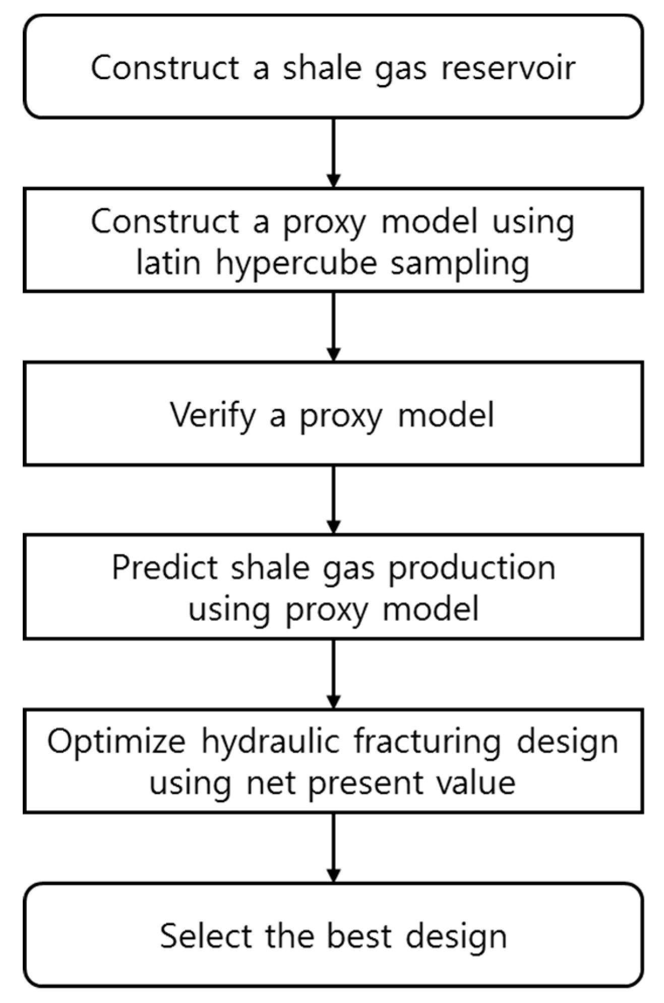
2. Methodology
2.1. Robust Regression for the Proxy Model
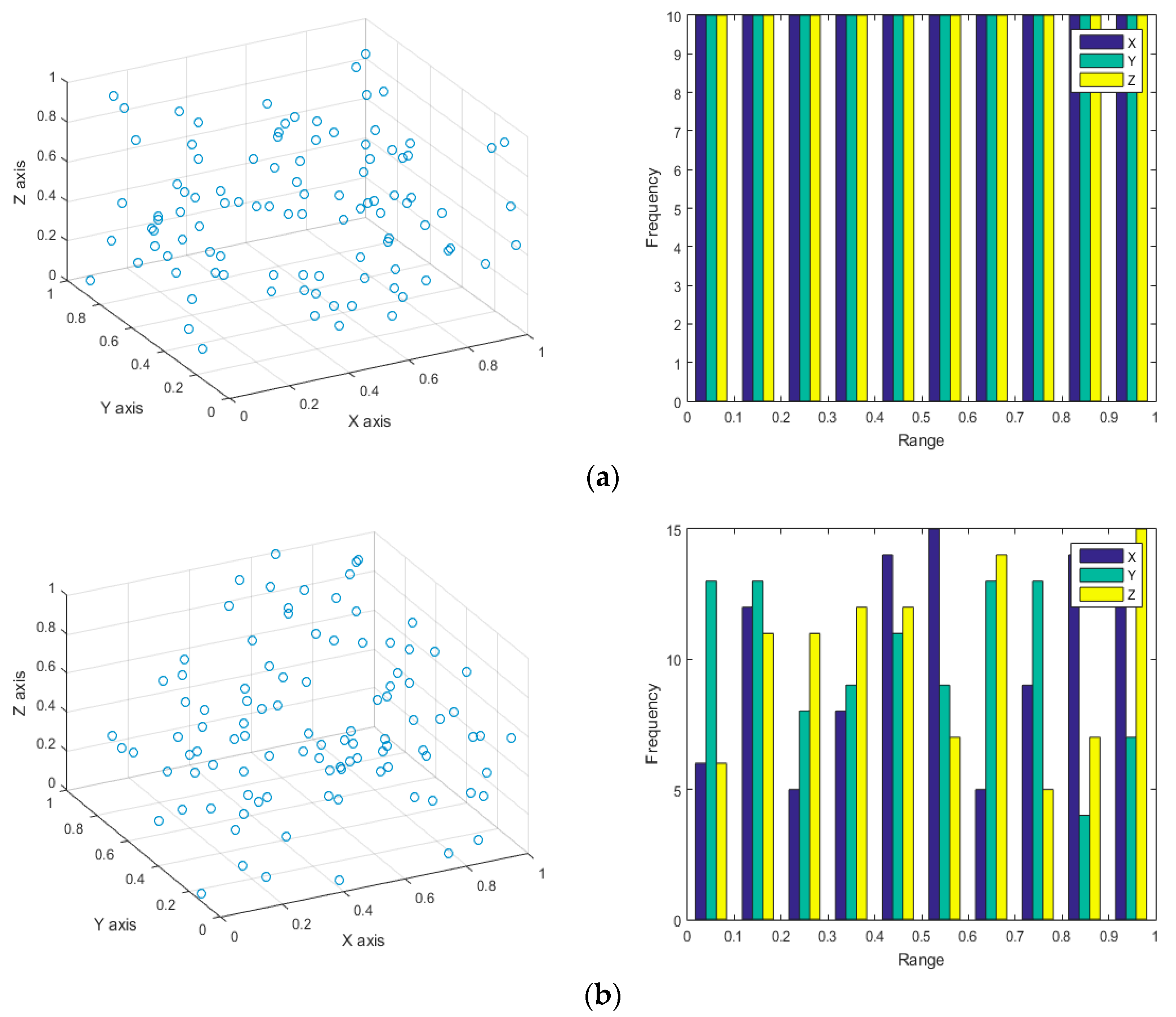
2.2. Latin Hypercube Sampling
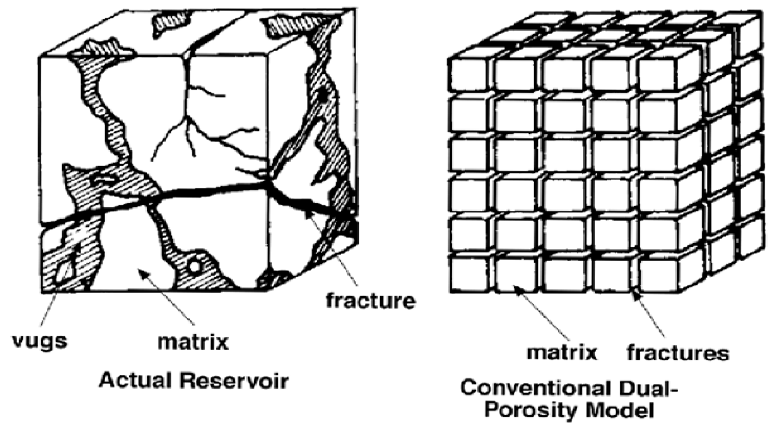
2.3. Dual Porosity–Dual Permeability Model
2.4. Net Present Value
3. Results and Discussion
3.1. Computation of the Proxy Model
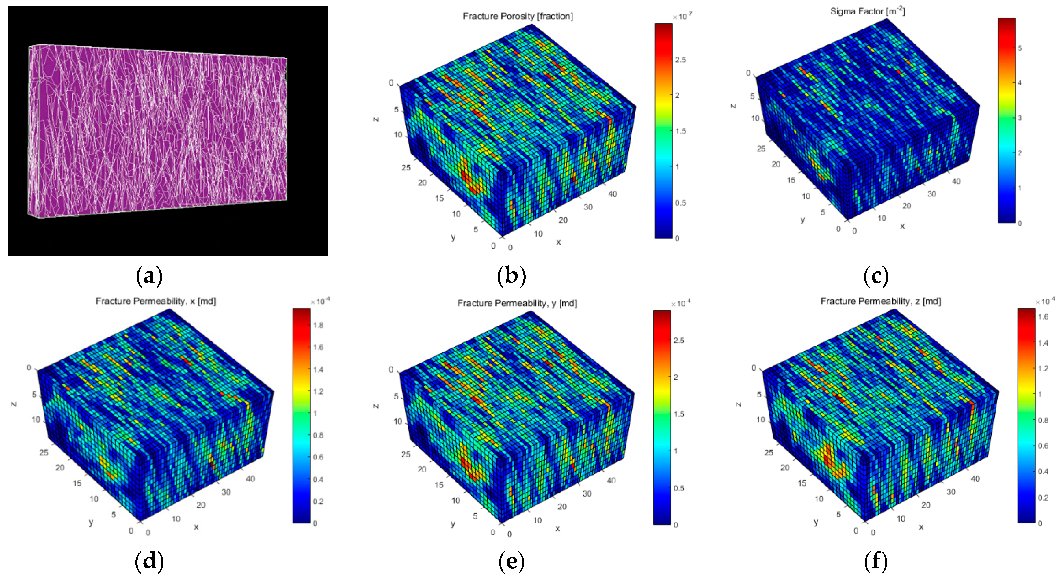
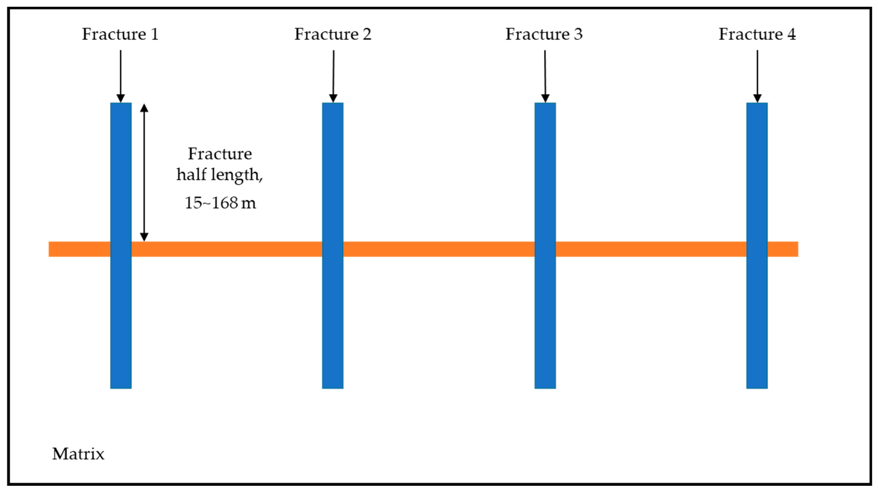
3.1.1. Modeling of the Unconventional Shale Reservoir
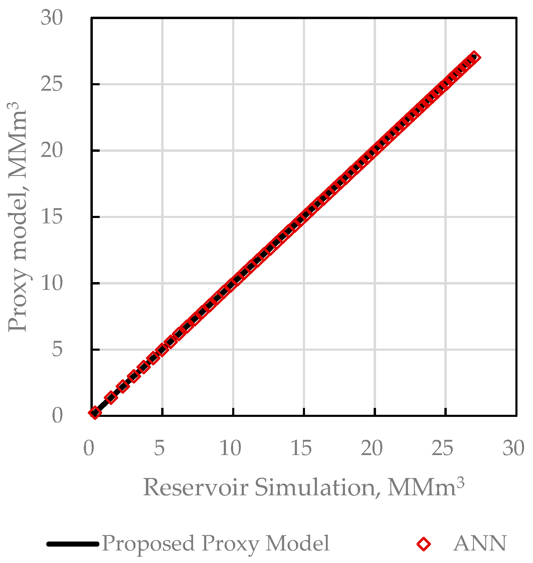
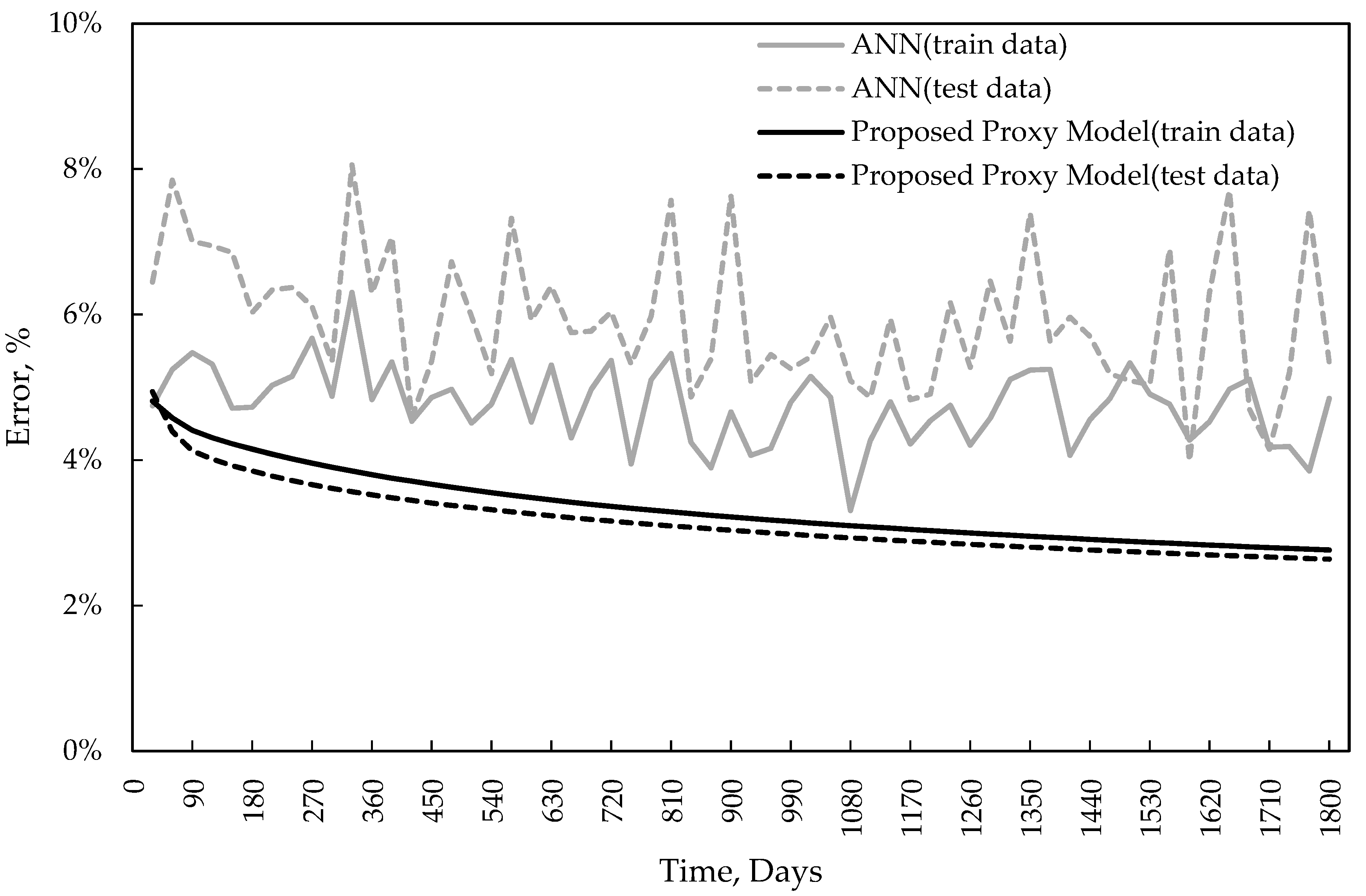
3.1.2. Proxy Model Based on the Robust Regression
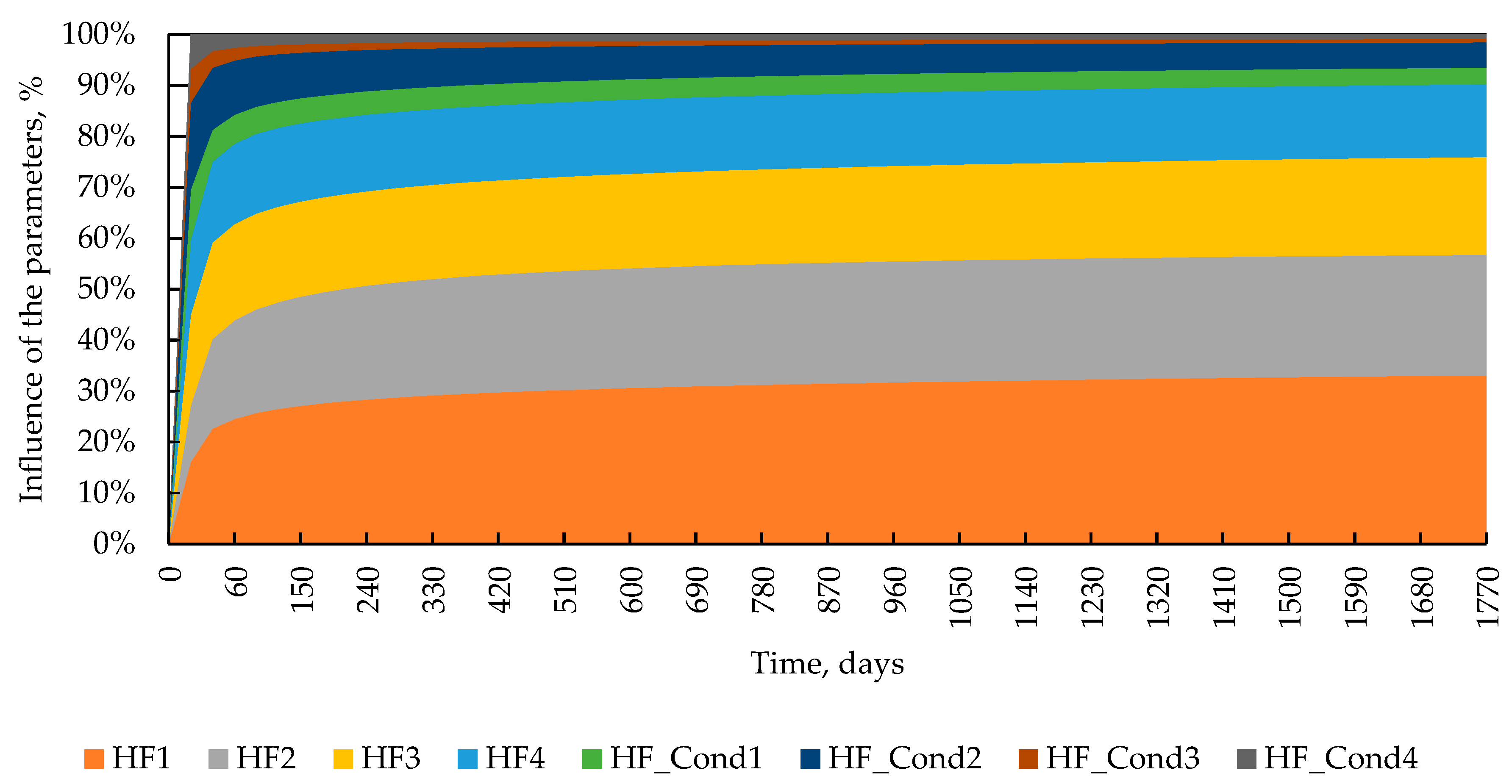
3.1.3. Sensitivity Analysis Using the Proxy Model
3.2. Optimization of Hydraulic Fracture Design
3.2.1. Assumptions for NPV Calculation
3.2.2. Results of Hydraulic Fracture Design
4. Conclusions
Author Contributions
Funding
Acknowledgments
Conflicts of Interest
References
- Mayerhofer, M.J.; Lolon, E.P.; Youngblood, J.E.; Heinze, J.R. Integration of Microseismic Fracture Mapping Results with Numerical Fracture Network Production Modeling in the Barnett Shale. In Proceedings of the SPE Annual Technical Conference, Richardson, TX, USA, 24–27 September 2006. [Google Scholar]
- Cipolla, C.L.; Lolon, E.P.; Mayerhofer, M.J.; Warpinski, N.R. Fracture Design Considerations in Horizontal Wells Drilled in Unconventional Gas Reservoirs. In Proceedings of the SPE Hydraulic Fracturing Technology Conference, The Woodlands, TX, USA, 19–21 January 2009. [Google Scholar]
- Valko, P.P.; Lee, W.J. A better way to forecast production from unconventional gas wells. SPE J. 2010, 2, 134–231. [Google Scholar]
- Biswas, D. Shale Gas Predictivie Model (SPGM)—An Alternate Approach to Predict Shale Gas Production. In Proceedings of the SPE Eastern Regional Meeting, Columbus, OH, USA, 17–19 August 2011. [Google Scholar]
- Yu, W.; Sepehrnoori, K. Optimization of Multiple Hydraulically Fractured Horizontal Wells in Unconventional Gas Reservoirs. In Proceedings of the SPE Production and Operations Symposium, Oklahoma City, OK, USA, 23–26 March 2013. [Google Scholar]
- Xie, J.; Yang, C.; Gupta, N.; King, M.J.; Datta-Gupta, A. Integration of Shale-Gas-Production Data and Microseismic for Fracture and Reservoir Properties with the Fast Marching Method. SPE J. 2015, 20, 347–359. [Google Scholar] [CrossRef]
- Kim, K.; Ju, S.; Ahn, J.; Shin, H.; Shin, C.; Choe, J. Determination of key parameters and hydraulic fracture design for shale gas productions. In Proceedings of the Twenty-fifth International Ocean and Polar Engineering Conference, Kona, HI, USA, 21–26 June 2015. [Google Scholar]
- Balan, H.O.; Gupta, A.; Georgi, D.T.; Al-Shawaf, A.M. Optimization of well and hydraulic fracture spacing for tight/shale gas reservoirs. In Proceedings of the Unconventional Resources Technology Conference, San Antonio, TX, USA, 1–3 August 2016. [Google Scholar]
- Kim, J.; Kang, J.; Park, C.; Park, Y.; Park, J.; Lim, S. Multi-Objective History Matching with a Proxy Model for the Characterization of Production Performances at the Shale Gas Reservoir. Energies 2017, 10, 579. [Google Scholar] [CrossRef]
- Tang, C.; Chen, X.; Du, Z.; Yue, P.; Wei, J. Numerical Simulation Study on Seepage Theory of a Multi-Section Fractured Horizontal Well in Shale Gas Reservoirs Based on Multi-Scale Flow Mechanisms. Energies 2018, 11, 2329. [Google Scholar] [CrossRef]
- Andersen, R. Modern Methods for Robust Regression; Sage Publications: London, UK, 2008. [Google Scholar]
- Mckay, M.D.; Beckmann, R.J.; Conover, W.J. A Comparison of Three Methods for Selecting Values of Input Variables in the Analysis of Output from a Computer Code. Technometrics 1979, 21, 239–245. [Google Scholar]
- Warren, J.E.; Root, P.J. The Behavior of Naturally Fractured Reservoirs. J. Soc. Pet. Eng. 1963, 3, 245–255. [Google Scholar] [CrossRef]
- Kazemi, H.; Merrill, L.S.; Porterfield, K.L.; Zeman, P.R. Numerical Simulation of Water-Oil Flow in Naturally Fractured Reservoirs. J. Soc. Pet. Eng. 1976, 4, 464–470. [Google Scholar] [CrossRef]
- Duguid, J.O.; Lee, P.C.Y. Flow in Fractured Porous Media. J. Water Resour. Res. 1977, 13, 558–566. [Google Scholar] [CrossRef]
- Schweitzer, R.; Bilgesu, H.I. The Role of Economics on Well and Fracture Design Completions of Marcellus Shale Wells. In Proceedings of the SPE Eastern Regional Meeting 2009, Charleston, WV, USA, 23–25 September 2009. [Google Scholar]
- US Energy Information Administration (EIA). Available online: https://www.eia.gov/dnav/ng/ng_pri_sum_dcu_nus_m.htm (accessed on 21 October 2018).


| Input Parameters (unit) | Fixed Value | Uncertain Value |
|---|---|---|
| Depth (m) | 2591 | – |
| Reservoir size (x, y, z) (m) | (899, 411, 79) | – |
| Grid size (∆x, ∆y, ∆z) (m) | (15, 15, 6) | – |
| Reservoir pressure (MPa) | 27.58 | – |
| Bottomhole pressure (MPa) | 3.45 | – |
| Diffusion coefficient (m2/day) | 0.0047 | – |
| Langmuir adsorption constant (1/kPa) | 0.0073 | – |
| Gas composition CH4 (%) | 100 | – |
| Rock density (kg/m3) | 1922.22 | – |
| Rock compressibility (1/MPa) | 0.00015 | – |
| Reservoir temperature (°C) | 25 | – |
| Number of hydraulic fracture stages | 4 | – |
| Average of matrix permeability (md) | 5.82 × 10⁻⁴ | – |
| Average of matrix porosity (fraction) | 0.037 | – |
| Hydraulic fracture half-length (m) | – | (15–168) |
| Hydraulic fracture conductivity (md·cm) | – | (305–1524) |
| Type | MAPE | R2 |
|---|---|---|
| ANN (training data) | 4.80% | 0.988 |
| ANN (testing data) | 6.00% | 0.980 |
| Proposed Model (training data) | 3.40% | 0.995 |
| Proposed Model (testing data) | 3.20% | 0.996 |
| Input Parameters (unit) | Value |
|---|---|
| Trend (degree) | 85 |
| Plunge (degree) | 15 |
| Fisher constant | 25 |
| Fracture length (m) | Lognormal (52, 9) |
| Fracture intensity (m2/m3) | 0.49 |
| Model | Enhanced Baecher |
| Trend (degree) | 85 |
| Horizontal Well Length (m) | Cost ($) | Hydraulic Fracture Half-Length per Stage (ft) | Cost ($) | Economic Parameter | Value |
|---|---|---|---|---|---|
| 305 | 2,000,000 | 76 | 100,000 | Operating cost | 30 $/day |
| 610 | 2,100,000 | 152 | 125,000 | Gas price 1 | 4.08 $/Mscf |
| 915 | 2,200,000 | 228 | 150,000 | Royalty | 12.5% |
| 1220 | 2,300,000 | 304 | 175,000 | Interest rate | 15% |
© 2019 by the authors. Licensee MDPI, Basel, Switzerland. This article is an open access article distributed under the terms and conditions of the Creative Commons Attribution (CC BY) license (http://creativecommons.org/licenses/by/4.0/).
Share and Cite
Kim, K.; Choe, J. Hydraulic Fracture Design with a Proxy Model for Unconventional Shale Gas Reservoir with Considering Feasibility Study. Energies 2019, 12, 220. https://doi.org/10.3390/en12020220
Kim K, Choe J. Hydraulic Fracture Design with a Proxy Model for Unconventional Shale Gas Reservoir with Considering Feasibility Study. Energies. 2019; 12(2):220. https://doi.org/10.3390/en12020220
Chicago/Turabian StyleKim, Kyoungsu, and Jonggeun Choe. 2019. "Hydraulic Fracture Design with a Proxy Model for Unconventional Shale Gas Reservoir with Considering Feasibility Study" Energies 12, no. 2: 220. https://doi.org/10.3390/en12020220
APA StyleKim, K., & Choe, J. (2019). Hydraulic Fracture Design with a Proxy Model for Unconventional Shale Gas Reservoir with Considering Feasibility Study. Energies, 12(2), 220. https://doi.org/10.3390/en12020220