Photovoltaic Energy Yield Improvement in Two-Stage Solar Microinverters

Abstract

The focus in this paper is on the two-stage photovoltaic (PV) microinverters using a buck-boost dc/dc front-end converter. Wide input voltage range of the front-end converter enables operation under shaded conditions but results in mediocre performance in the typical voltage range. These microinverters can be controlled with either fixed or variable dc-link voltage control methods. The latter improves the converter efficiency considerably in the range of the most probable maximum power point (MPP) locations. However, the buck-boost operation of the front-end converter results in noticeable variations of the efficiency across the input voltage range. As a result, conventional weighted efficiency metrics cannot be used to predict annual energy productions by the microinverters. This paper proposes a new methodology for the estimation of annual energy production based on annual profiles of the solar irradiance and ambient temperature. Using this methodology, quantification of the annual energy production is provided for two geographical locations.

1. Introduction

In the recent year, residential solar photovoltaic (PV) systems have been on the rise, resulting from strong governmental support either in the form of subsidies on installation or feed-in tariffs [1,2,3,4]. This trend has been supported with the rapid cost reduction of PV modules and associated hardware [5]. Deployment of PV systems relies on extensive use of power electronic converters as the critical system components [6]. Residential applications are mostly associated with either string inverters or microinverters [7]. The latter could be regarded as the class of module-level power electronic (MLPE) systems [8]. Another member of this class is PV power optimizers used for interfacing individual PV modules in series PV string and, thus, they bridge the gap between string inverters and microinverters. However, they impose limitations on system design due to voltage matching issues.

Residential PV systems are usually built with string inverters for systems over 1 kW of installed power to optimize installation costs. However, series connection of PV modules into string results in relatively high dc voltage operating on the roof. Any issues with mechanical contacts within a PV string can easily result in dc arcing and, consequently, fire hazard. In addition, a PV string inverter can be considered as a single point of failure reducing overall reliability. Moreover, the 2017 National Electrical Code was revised in section 690.12, which discards array level rapid shut-down requirements and imposes PV module-level rapid shut-down requirements [9]. Starting from 2019, this regulation requires that voltage of all conductors be dropped below 80 V within 30 s from rapid shutdown initiation. As a result, string PV systems require use of smart modules or PV power optimizers along with a PV string inverter, which makes them comparable in price to systems with a microinverter, but more labor intensive to install.

Shading of PV modules is a serious issue in residential PV systems [10,11]. Conventional string PV inverters cannot withstand harsh shading conditions due to their limited voltage regulation capability. In such cases, MLPE converters have to be used to optimize the maximum power point (MPP) tracking (MPPT) process under shading conditions [7]. PV power optimizers could be advantageous in larger residential PV systems due to the possibility of selective deployment. However, they can ensure proper maximum energy harvesting by a PV string inverter only for a limited number of PV string configurations containing a number of modules within a certain range [12]. Contrary to that, microinverters accomplish parallel grid integration of individual PV modules into the grid. Hence, rapid PV module-level shutdown is ensured. Other advantages of the microinverters, PV module health monitoring, and dust accumulation detection, are provided; flexible PV system design is possible [7].

PV microinverters can be regarded as a universal tool for deployment of small residential PV systems, which provides superior scalability and reliability [7]. Usually, they are based on either single- or two-stage energy conversion. The former features low cost of implementation at the expense of regulation range limitations, while the latter is a more complex solution with a wider input voltage regulation range. The two-stage solutions are approaching the input voltage range of the PV power optimizers. PV power optimizers usually feature a wide input voltage range of 8 to 55 V to accommodate partial shading, when the global MPP voltage can be as low as one third of the unshaded MPP voltage for conventional Si PV modules with three bypass diodes. Hence, single-stage microinverters cannot withstand opaque or significant partial shading and thus must be replaced with two-stage solutions in climatic conditions where shading causes energy yield loss.

2. DC Link Voltage Control in Two-Stage PV Microinverters

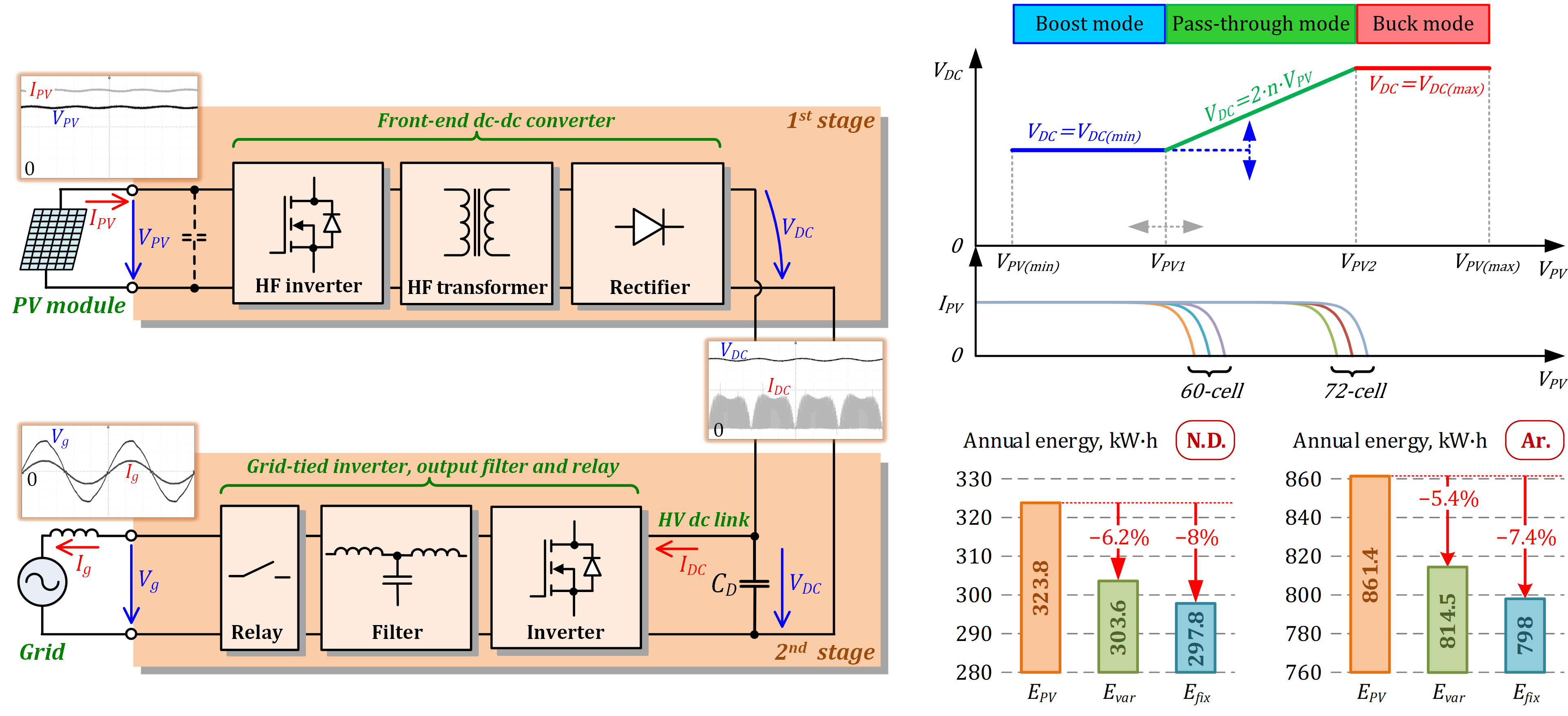
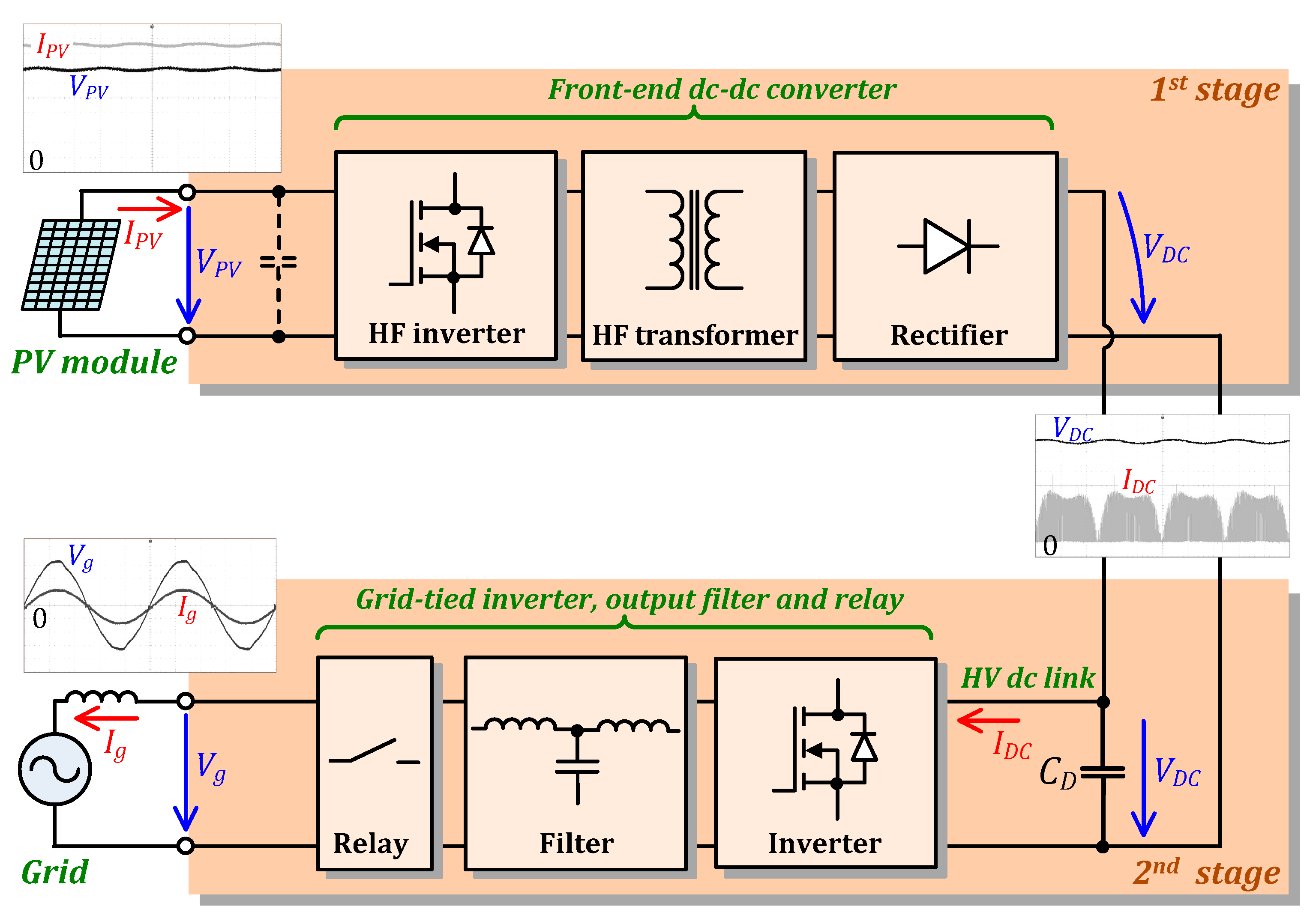
A typical two-stage PV microinverter (Figure 1) is comprised of a front-end dc/dc converter that ensures decoupling of 100/120 Hz ripple from the input port while enabling converter operation at partial and opaque shading of a PV module. The latter feature is usually realized with the application of a galvanically isolated buck-boost dc/dc converter [13] at the input. Recently, several converters based on this concept were justified as high-performance MLPE solutions [14,15,16]. They can include separate buck and boost switching cells [13,14], as well as a single integrated buck-boost switching cell [15,16].

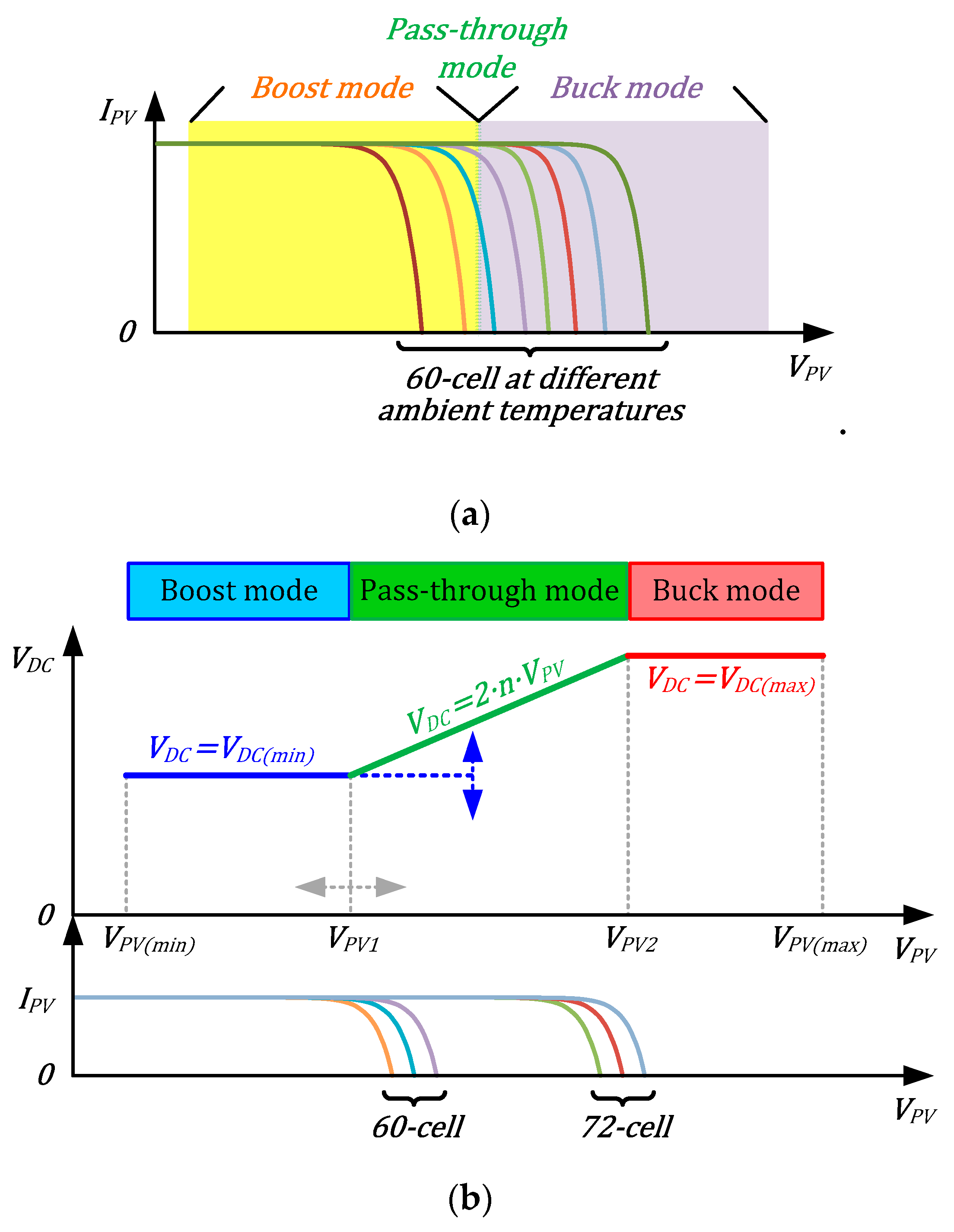
Typically, a buck-boost front-end dc/dc converter features three operation modes used for the input voltage regulation: buck, boost, and pass-through. The latter mode is the most efficient among the three as a converter does not perform voltage regulation and operates as a dc transformer (DCX). In the MLPE applications, the dc-link voltage is often fixed. In such a case, the isolating high-frequency (HF) transformer has to be designed to ensure that the pass-through mode coincides with the most probable maximum power point (MPP), as shown in Figure 2a. As a result, the buck mode is utilized during the microinverter start-up or MPPT that starts from the open-circuit voltage, as well as in the operation at low ambient temperatures when a PV module features elevated operating voltages. At the same time, the boost mode comes in handy at high ambient temperatures, when the MPP voltage of a PV module is reduced, as well as at shaded conditions to optimize the MPPT.

The dc-link voltage does not necessarily have to be fixed since the grid-side inverter enables this additional degree of control freedom. In this case, a microinverter operates in the boost mode at very low voltages that correspond to partial or opaque shading conditions and the dc-link voltage is limited at the minimum required value V_DC(min), i.e., 10 V, …, 20 V above the instantaneous grid peak voltage. The pass-through mode featuring the maximum efficiency corresponds to the most probable range of MPPs, while the grid-side inverter should perform the MPP tracking. The buck mode is used for the MPPT tracking or operating at low ambient temperatures. The dc-link voltage in the buck mode is maximum allowed by the voltage rating of the dc-link capacitor and grid-side inverter switches. Such an arrangement can result in efficient operation with the most typical Si PV modules containing 60- and 72-cell (Figure 2b). Recently, the variable dc-link voltage control was applied in several state-of-the-art two-stage microinverters [17,18] and battery chargers [19]. It resulted in higher efficiencies, extended reliability, and good compatibility with different PV modules [20,21].

The variable dc-link voltage control optimizes the efficiency of the two-stage microinverter but results in sizable variations of the efficiency around transitions between the pass-through mode and the buck or the boost mode. As a result, standardized weighted efficiencies, such as California Energy Commission (CEC) or EU metrics, would be of no use for predictions of the annual energy production by the two-stage buck-boost microinverters as their efficiency depends on the operating voltage considerably or it has to be added in the specifications. This study proposes a methodology for annual energy production estimation for the aforementioned microinverters and provides a numerical study based on experimental data to quantify the effect on converter efficiency achieved when the fixed dc-link voltage control is replaced with the variable dc-link voltage control.

3. Case Study Microinverter and Experimental Results

The microinverter for this study is described in detail in [18]. Its topology is shown in Figure 3 and the main specifications are listed in

Table 1. Prototype parameters and components.

Parameter or Component	Symbol or Block		Type or Value
Transformer	TX	N	6
		Llk	25 μH
		Lm	1000 μH
QZS inductor	LqZS	LlkqZS	0.5 μH
		LmqZS	11 μH
QZS capacitors	CqZS1, CqZS2		12 × 2.2 μF (X7R/100 V)
Resonant capacitors	C1, C2		43 nF (foil)
Dc-link capacitor	CD		150 μF (Al electrolytic)
LCL filter	Lf1		2.6 mH
	Lf2		1.8 mH
	Cf		0.47 μF
Fix. dc-link voltage	VDC		400 V
VAr dc-link voltage	VDC(min)		335 V
	VDC(max)		460 V
Grid	Vg		230 V/50 Hz
Switching frequency	SqZS		210 kHz
	S1…S4		105 kHz
	S5, S6		50 Hz
	S7, S8		20 kHz
LV semiconductors	SqZS, S1…S4		Infineon BSC035N10NS5
HV semiconductors	D1, D2		Wolfspeed C3D02060E
	S5, S6		Infineon IPB60R099C7
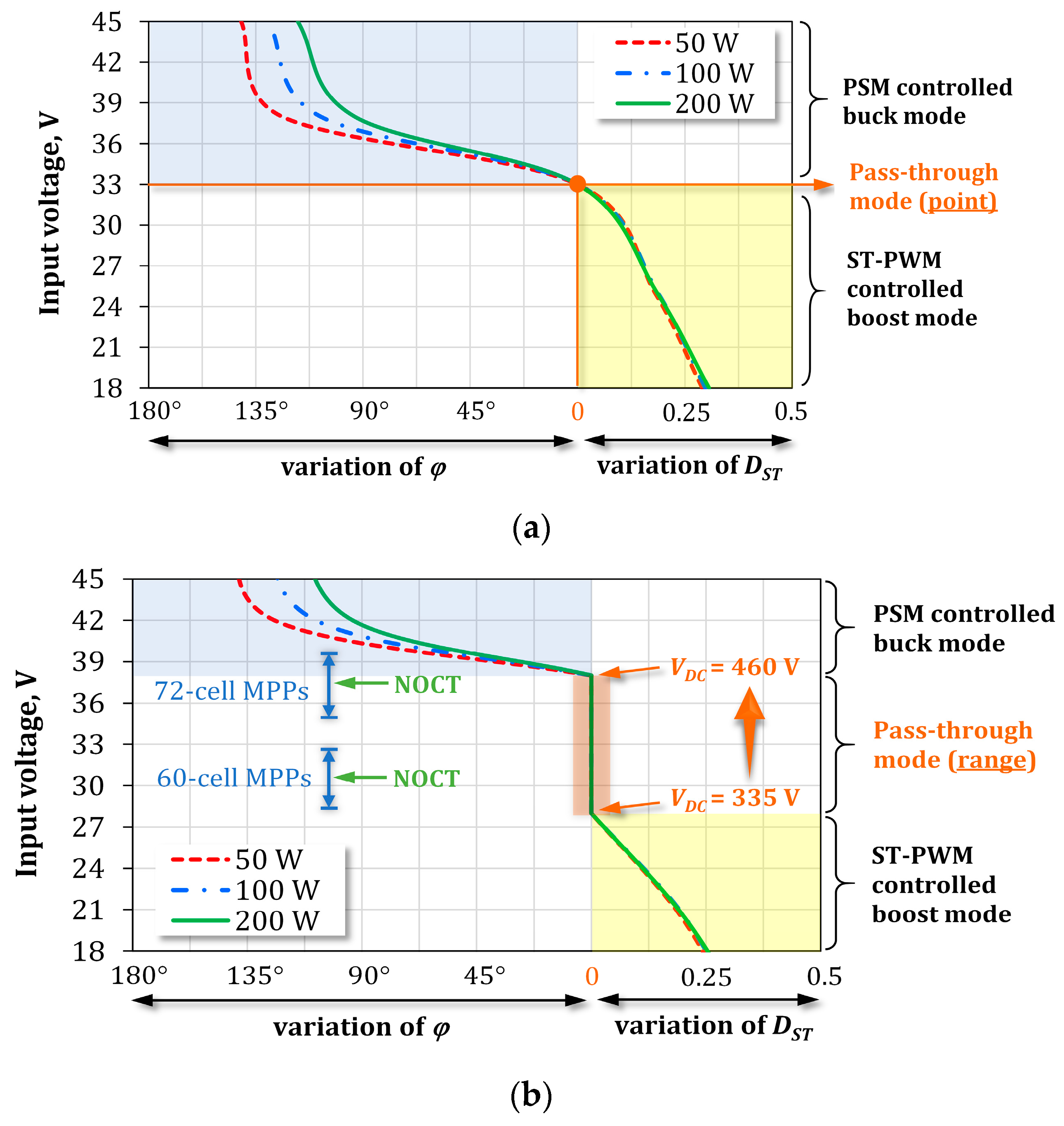
	S7, S8		ROHM SCT2120AFC

. The front-end dc/dc converter utilizes the hybrid quasi-Z-source series resonant topology. The front-end dc/dc converter implements the boost mode using the shoot-through pulse width modulation (ST-PWM) implemented by the symmetrical overlap of active states with the duty cycle D_ST. As a result, the input quasi-Z-source network can store energy and use it for the input voltage step-up. In the pass-through mode, it operates as the series resonant converter with very high efficiency. The grid-side inverter has to perform MPPT when the front-end dc/dc converter operates in the pass-through mode. The front-end dc/dc converter utilizes phase-shifted modulation (PSM) with an angle φ to implement voltage buck using the integrated series resonant tank. Two different dc-link voltage control principles result in a fundamentally different operation of the front-end converter, as shown in Figure 4. At the variable dc-link voltage, the region of the highest efficiency coincides with the most probable MPPs of 60- and 72-cell Si PV modules, i.e., when they operate under nominal operating cell temperature (NOCT).

The given two-stage microinverter topology [18] was selected as it has shown a wide input voltage range of over 1:6, which is wider than any other competitor and was justified as a shade-tolerant solution capable of withstanding the worst shading conditions.

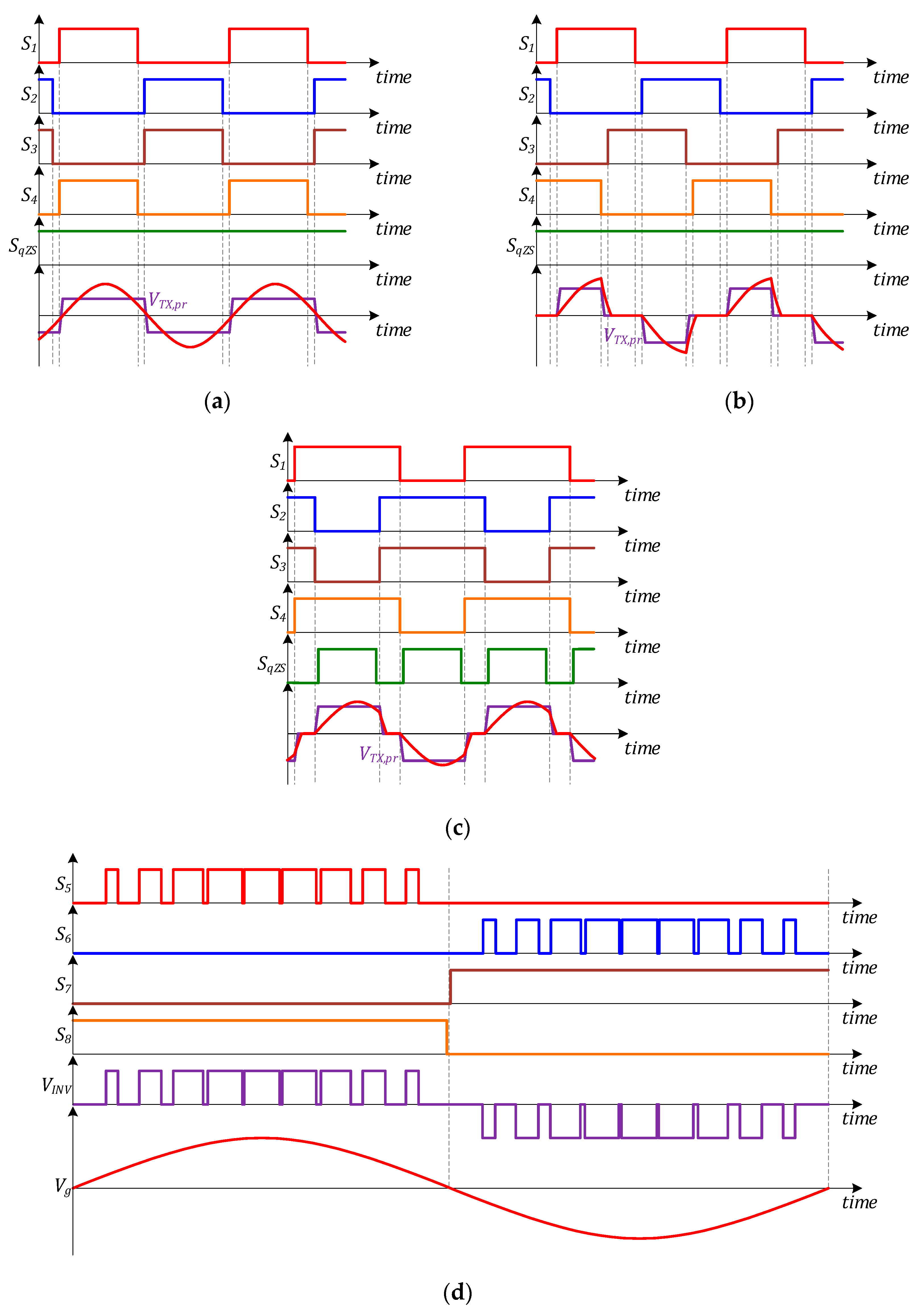
Figure 5 presents the modulation techniques used in the case study microinverter. Modulations of the front-end dc/dc converter and the grid-tied inverter are decoupled and are not synchronized in a general case. The front-end dc/dc converter operates at relatively high switching frequency in order to minimize the size of the isolation transformer, resonant tank, etc. The switch S_qZS is turned ON continuously in the buck and pass-through mode, as shown in Figure 5a,b. The carrier frequency of the switches S_1, …, S₄ is 105 kHz [15,18]. On the other hand, the switch S_qZS operates at a switching frequency twice higher than that of the switches S₁…S₄ as it is active during active states when the isolation transformer is fed with voltage pulses (Figure 5c). Detailed description of the dc/dc converter operation is provided in [15].

The grid-tied inverter utilizes asymmetrical unipolar modulation shown in Figure 5d. In this modulation, two switches operate at high frequency (carrier frequency of the S₅, S₆ PWM signals is 20 kHz in the given case), while the other two switches S₇, S₈ operate at the grid frequency and unfold the grid voltage. This modulation was selected despite uneven losses in the switches as it provides 50 Hz rectangular common mode voltage and thus ensures low leakage current and good electromagnetic compatibility, as demonstrated in [18], where full operation of the microinverter is presented along with the description of the closed-loop control system.

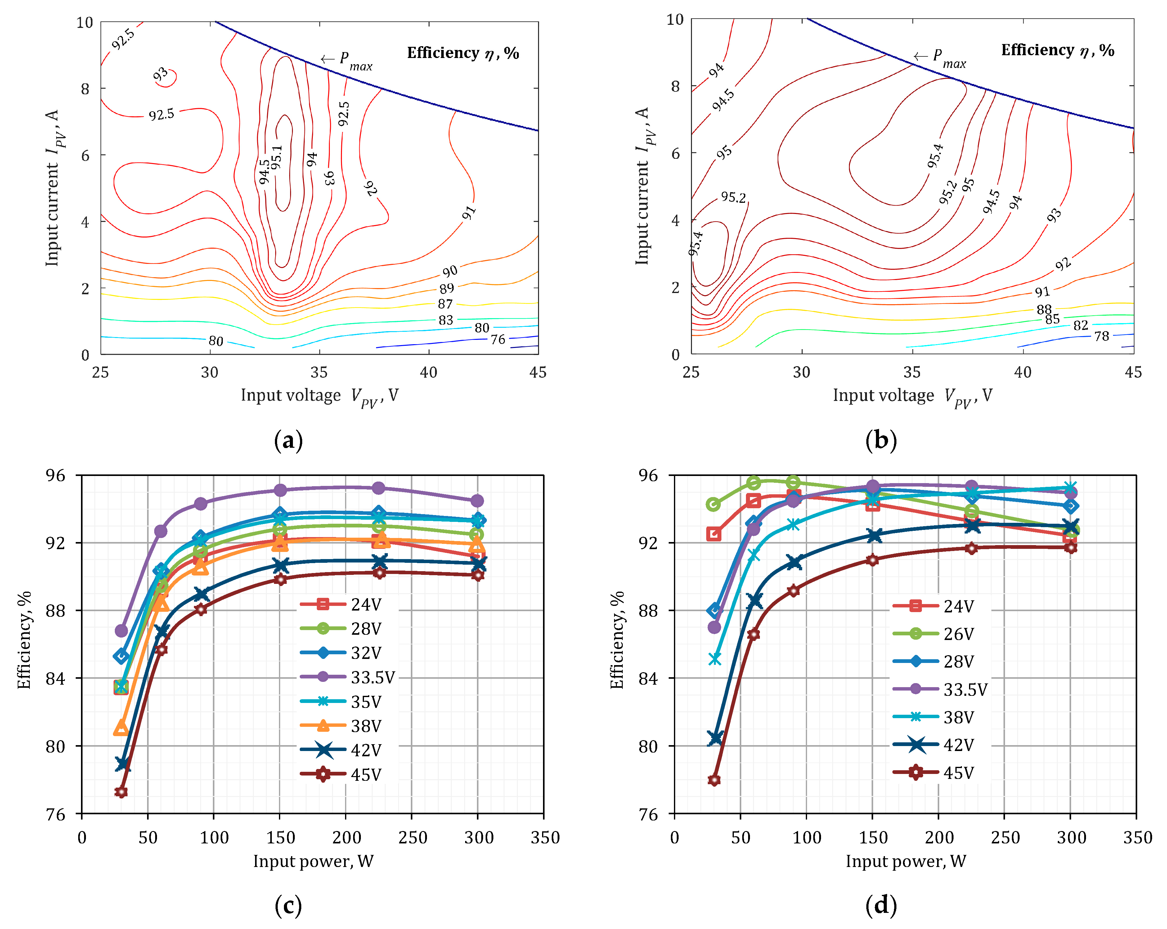
The efficiency of the experimental prototype was measured for both dc-link voltage control methods in the input voltage range of 25 to 45 V and from 10% to 100% of the rated power of 300 W. The rated power was selected during design to satisfy the requirements of the given application as will be shown in the next section. Over 50 reference points were acquired using a precision power analyzer Yokogawa WT1800. Next, the experimental efficiency surfaces were obtained in MATLAB using the surface fitting tool and thin-plate spline for interpolation. The contour plots of the experimental data interpolation shown in Figure 6a,b follow tightly the experimental data in Figure 6c,d, which results in the coefficient of determination (R²) equal to unity. This data will be used further for annual performance prediction. It can be seen from Figure 6 that the fixed dc-link voltage control results in a limited region of high efficiency where the front-end dc/dc converter operates in or close to the pass-through mode. At the same time, the variable dc-link voltage control extends the region of the pass-through mode usage, which results in roughly 2% higher efficiency across the considered operation range.

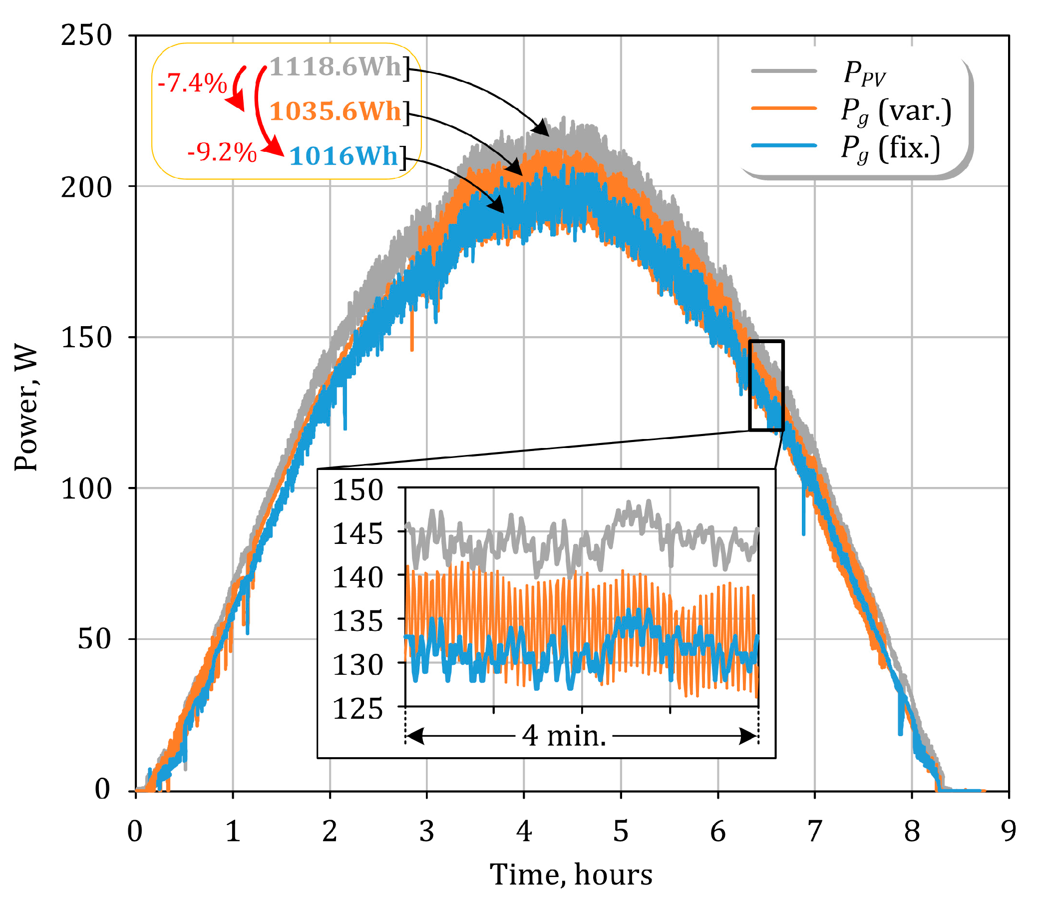
To provide an experimental example of PV energy harvesting by the case study microinverter, one-day operation (moderate irradiance and no clouds) was simulated using a PV simulator Chroma 62150H-1000S. According to Figure 7, the variable dc-link voltage results in higher power injected in the grid than that for the fixed dc-link voltage control. It improves the overall efficiency of the former, thus, reducing the loss of the available PV energy from 9.2% to 7.4%, i.e., reducing the energy loss by 19.6%. This study considers the efficiency of the microinverter and leaves the MPPT efficiency out for simplicity.

4. Estimation of Annual PV Energy Production

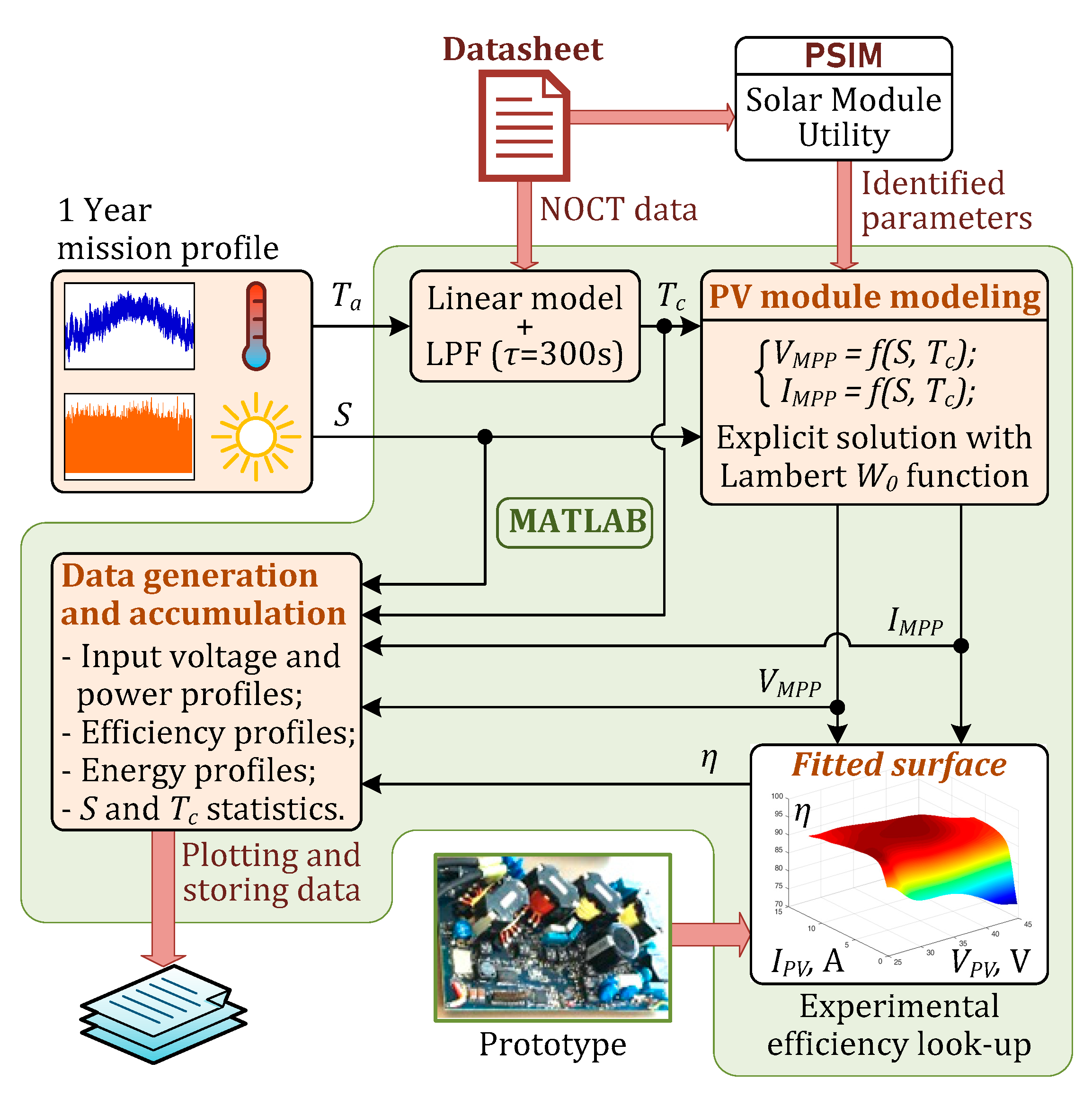
The interpolations of the experimental efficiency (Figure 6) can be used to estimate the annual energy production and energy loss for the two dc-link control methods. The efficiency includes microinverter self-powering from the input PV power. The developed methodology is explained in Figure 8. It utilizes 1-year mission profiles of the solar irradiance and the ambient temperature for Arizona (Ar.) and North Denmark (N.D.) [22] with a 1-minute resolution.

First, the ambient temperature (T_a) is translated into the cell temperature (T_c) using a simple linear model with a low-pass filter to account for the thermal dynamics of a PV module:

$$T_c=\left[T_a+\frac{T_{NOCT}-T_{a(NOCT)}}{S_{NOCT}}\cdot S\right]\cdot G_{LPF}(s),$$

(1)

where the nomenclature is listed

Table 2. Nomenclature.

Term	Explanation	Term	Explanation
kb	Boltzmann constant	vt	Thermal voltage
q	Elementary charge	Rs	Series resistance of PV module
a	Ideality factor	Rs(STC)	Rs in STC conditions
Eg	Band gap energy	krs	Rs thermal coefficient
Ta	Ambient temperature	Rsh	Shunt resistor of PV module
Tc	Cell temperature	I0(STC)	I0 in STC conditions
S	Solar irradiance	I0	Saturation current
TSTC	Tc in STC conditions	IPh	Photocurrent
SSTC	S in STC conditions	NS	Number of cells in PV module
Ta(NOCT)	Ta in NOCT conditions	η	Microinverter efficiency
SNOCT	Solar irradiance in NOCT condition	Pg	Microinverter output power
TNOCT	Nominal operating cell temperature (NOCT)	ISC(STC)	Short-circuit current of PV module in STC conditions
VMPP(id)	MPP voltage of ideal PV module	τ	Thermal time constant of PV module
IMPP(id)	MPP current of ideal PV module	W0(⋅)	Principle branch of Lambert W function
IPV	Microinverter input current	VMPP	Module MPP voltage
VPV	Microinverter input voltage	IMPP	Module MPP current
PPV	Microinverter input power	PMPP	Module MPP power

. G_LPF is the low pass filter transfer function in the s-domain:

$$G_{LPF}(s)=\frac{1}{1+s\cdot \tau }.$$

(2)

In the second stage, the PV module has to be simulated by the typical single-diode model of a PV cell (Figure 9) using five parameters described in [23,24,25].

In the given model of a PV cell, diode D plays a crucial role. The fundamental value defining the operation of the p-n junction in the diode is the thermal voltage v_t:

$$\{\begin{array}{l}{I}_D=I_0\cdot \left(e^{\frac{V_D}{a\cdot v_t}}-1\right);\\ v_t=\frac{T_c\cdot k_b}{q}.\end{array}.$$

(3)

According to Shockley’s expression [26], the diode current is proportional to the reverse bias saturation current defined as:

$$I_0=I_{0(STC)}\cdot {\left(\frac{T_c}{T_{STC}}\right)}^3\cdot e^{\left(\frac{q\cdot E_g}{a\cdot k_b}\right)\cdot \left(\frac{1}{T_{STC}}-\frac{1}{T_c}\right)}.$$

(4)

The given model differs from the conventional model in the approach of simulating the series resistance R_s. Recent reports show its positive thermal dependence based on experimental results [27]. The PV module Jinko Solar JKM300M-60B used in modeling is based on the monocrystalline silicon technology and contains 60 cells. For this type of modules, the experimental thermal coefficient of R_s (k_rs) was reported in [27] to be used in the following equation:

$$R_s=R_{s(STC)}\cdot \left(1+k_{rs}\left(T_c-T_{STC}\right)\right).$$

(5)

As was mentioned before, the operation of the diode D defines the output current and the voltage of a PV cell, but its current is limited by the photocurrent generated by a PV cell:

$$I_{Ph}=I_{SC(STC)}\cdot \frac{S}{S_{STC}}\cdot \frac{R_s+R_{sh}}{R_{sh}}.$$

(6)

Some of the equations above contain the PV cell voltage inside and outside the exponential function, which can be resolved only using the Lambert function (in this case, its principle branch denoted as W₀). For further calculations, a helper variable must be introduced in terms of the Lambert function:

$$w=W_0\left(\frac{I_{ph}\cdot e^1}{I_0}\right).$$

(7)

Using this variable, the MPP voltage and current could be derived for an ideal PV cell containing only a photocurrent source and a diode:

$$V_{MPP(id)}=Ns\cdot a\cdot v_t\cdot (w-1),$$

(8)

$$I_{MPP(id)}=I_0\cdot (w-1)\cdot e^{(w-1)}.$$

(9)

However, this estimation is inaccurate as the influence of the shunt and series resistors has to be taken into account [23]:

$$I_{MPP}=I_{MPP(id)}-\frac{V_{MPP(id)}}{R_{sh}},$$

(10)

$$V_{MPP}=V_{MPP(id)}-I_{MPP}\cdot R_s,$$

(11)

$$P_{MPP}=V_{MPP}\cdot I_{MPP}.$$

(12)

Equations (3) to (12) constitute a short description of the methodologies described in [23,24,25] based on the single-diode PV cell module, but enhanced with findings from [27]. In addition, the final calculations take into account material properties of silicon from [28] and typical PV module thermal characteristics from [29], which are listed in

Table 3. PV module parameters.

Model Parameters		Reference Data and Constants
Parameter	Value	Parameter	Value
SSTC	1000 W/m2	VMPP(STC)	32.6 V
TSTC	25 °C	IMPP(STC)	9.21 A
SNOCT	800 W/m2	VOC(STC)	40.1 V
TNOCT	45 °C	ISC(STC)	9.72 A
Ta(NOCT)	20 °C	VMPP(NOCT)	30.6 V
a [27]	1.1	IMPP(NOCT)	7.32 A
Eg [28]	1.12 eV	VOC(NOCT)	37.0 V
I0(STC)	5.39⋅10−10 A	ISC(NOCT)	8.01 A
Rsh	750 Ω	Efficiency	17.98%
Rs(STC)	0.228 Ω	Ns	60
krs [27]	0.356 %	kb	1.38⋅10−23 J/K
τ [29]	300 s	q	1.602⋅10−19 C

.

Third, it is possible to define the MPP power and voltage for any solar irradiance and cell temperature. Considering the interpolated efficiency of the microinverter η, and assuming a perfect MPPT when V_PV = V_MPP and P_PV = P_MPP, it is possible to define the microinverter output power P_g and, thus, the energy production E during an arbitrary time interval t_x:

$$P_g(t)=V_{MPP}(t)\cdot I_{MPP}(t)\cdot \eta \left(V_{MPP}(t);I_{MPP}(t)\right),$$

(13)

$$E={\displaystyle \underset{o}{\overset{t_x}{\int }}{P}_g(t)dt}.$$

(14)

Table 3 presents the parameters of the solar module obtained from the datasheet, PSIM Solar module utility, and other literature (for fundamental and empiric constants).

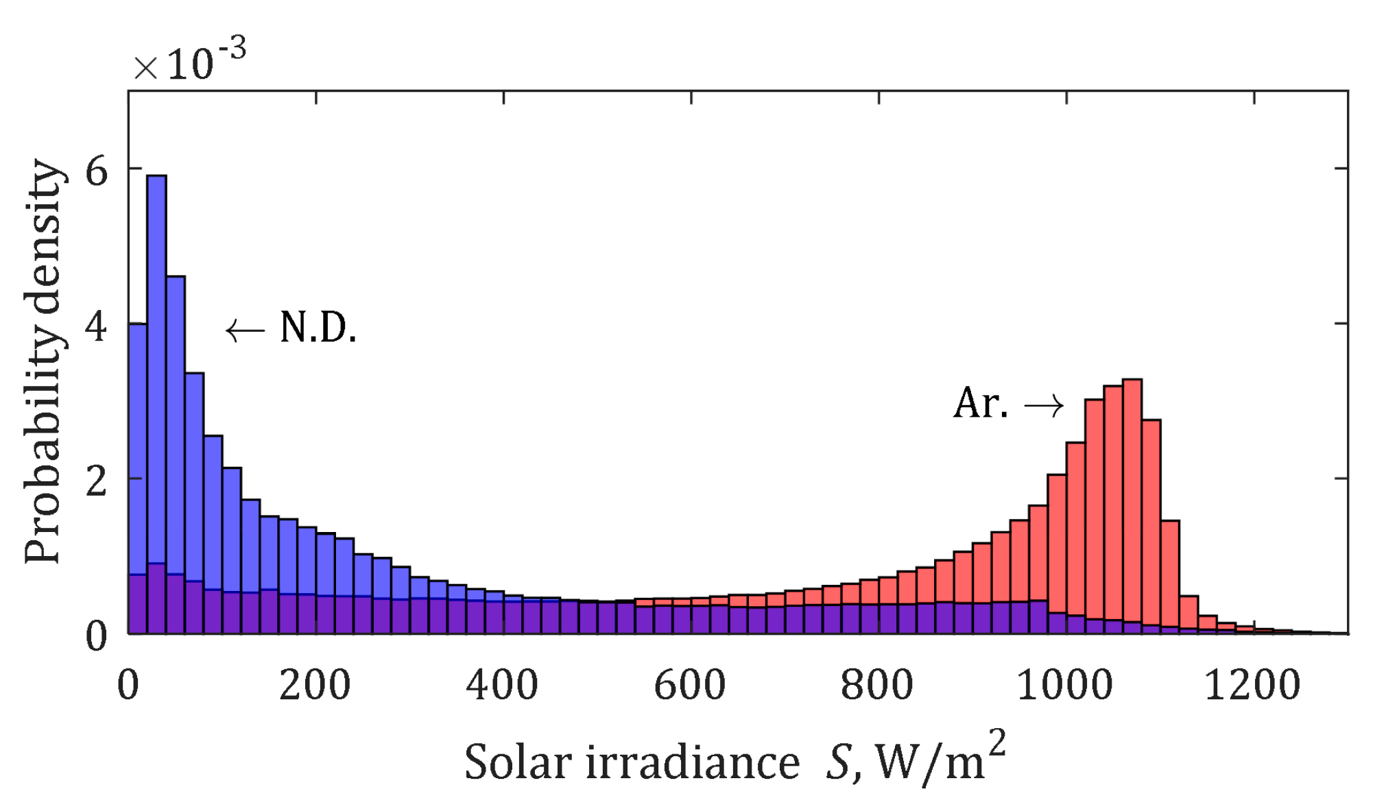
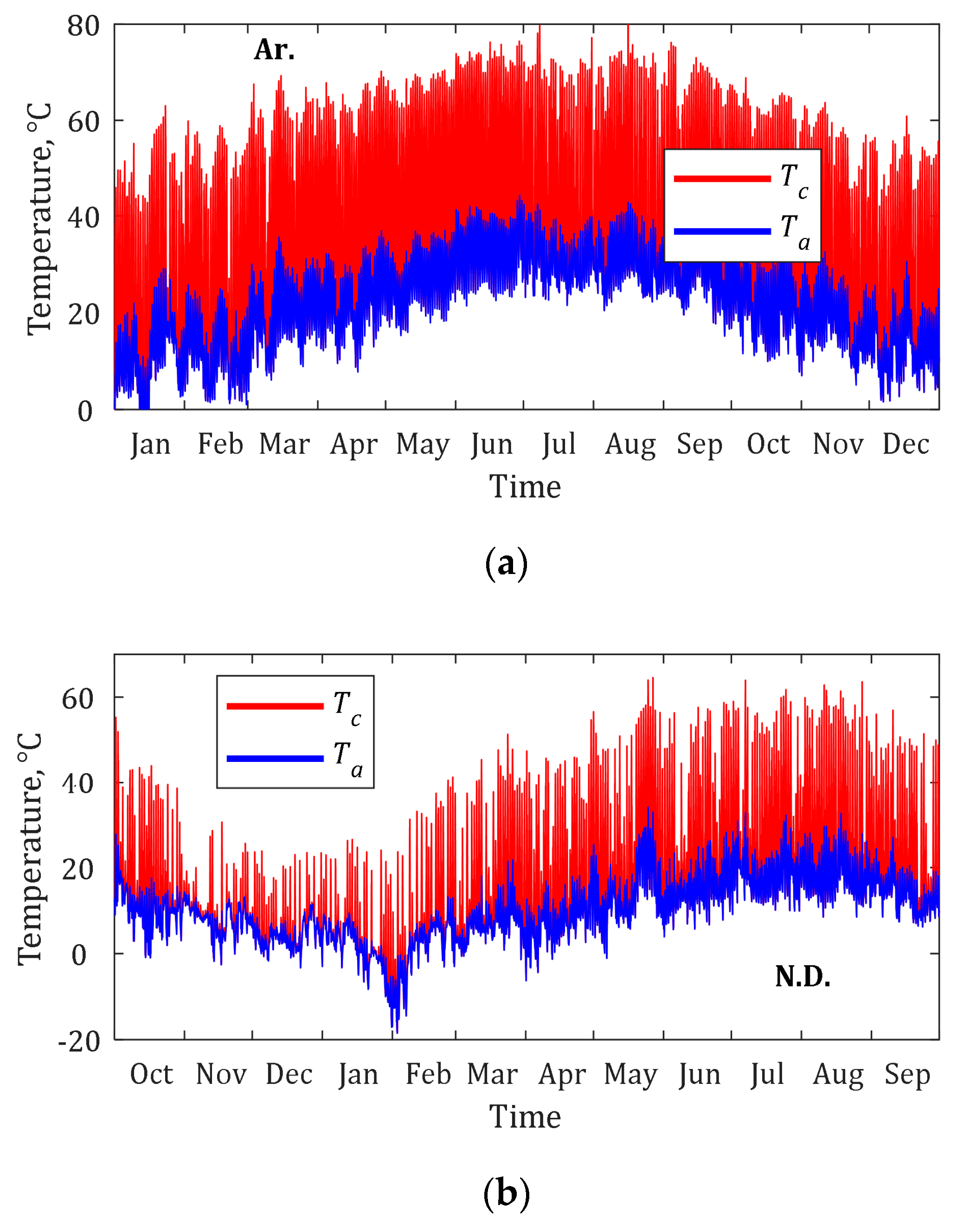
The considered geographic locations differ significantly in the operating conditions. Distribution of solar irradiance has a higher expectation around 1000 W/m² for Arizona and around 100 W/m² for North Denmark, as shown in Figure 10. As a result of higher solar irradiance and ambient temperature, the PV module will experience much higher thermal stress in Arizona conditions, which was calculated using Equation (1) and plotted in Figure 11. Probability density distribution of the cell temperatures shown in Figure 12 proves that the cell temperature is mostly between 10 °C and 75 °C in the Arizona conditions, contrary to the range of −5 °C to 60 °C in the North Denmark conditions, which is calculated ignoring night time.

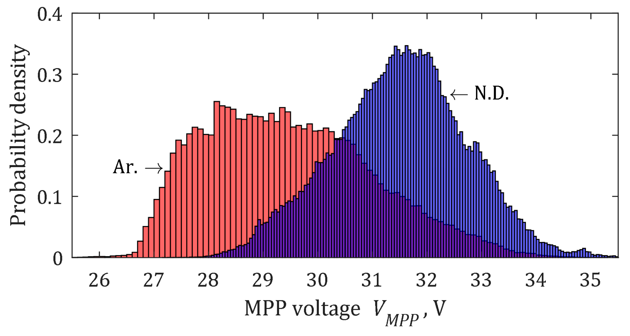
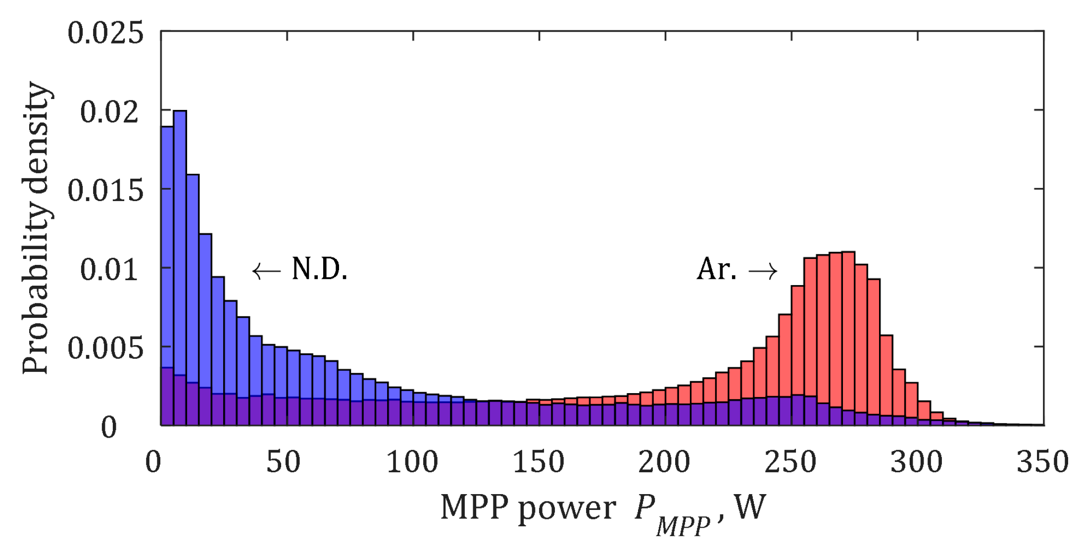
Next, annual mission profiles of solar irradiance and ambient temperature are translated into annual profiles of the MPP voltage and power using the model of the PV module described above. Probability distribution functions of these physical quantities are shown in Figure 13 and Figure 14. Lower cell temperatures and solar irradiance levels resulted in higher MPP voltages but lower average MPP power in the North Denmark conditions. Contrary to that, the microinverter will process higher powers at lower MPP voltages in the Arizona conditions.

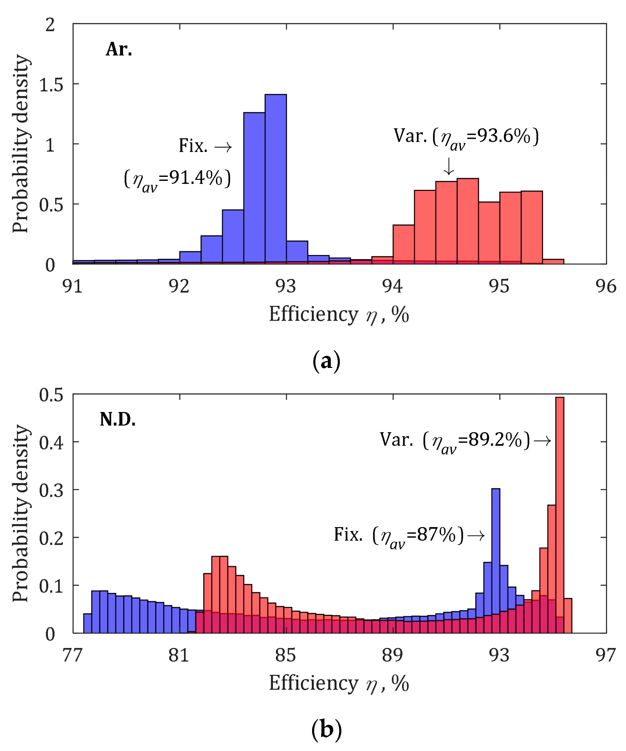
Annual mission profiles of the MPP voltage and power can be applied to the efficiency look-up block that performs interpolations for the experimental efficiency using thin-plate splines derived in MATLAB. The probability distribution of the efficiency of the microinverter strongly depends on the geographic location as well as on the dc-link voltage control. In the Arizona conditions, high average MPP power results in the narrow distribution range of 92% to 93.5% for the fixed dc-link voltage control and 94% to 95.5% for the variable dc-link voltage control, as it follows from Figure 15a. For the case of fixed dc-link voltage control, the values of efficiency can reach as low as 77% and as high as 95.2%. This wide distribution range results in a relatively low average efficiency of 91.4%. Contrary to that, in the North Denmark conditions, the microinverter will feature sizable probability values in a much wider range of efficiencies due to more intermittent solar irradiance, as shown in Figure 15b. Nevertheless, in both cases, the variable dc-link voltage control provides efficiencies higher by 2.2% on average than in the case of fixed dc-link voltage control.

Average values of the annual microinverter efficiency are not sufficient to reach any definitive conclusion regarding annual energy production as the efficiency values have to be weighted with the input power values.

Table 4. Annual energy production simulation results.

Location	North Denmark		Arizona
Dc-link Voltage Control	Fixed	Variable	Fixed	Variable
Usable PV energy, kW⋅h	323.8		861.4
Produced energy, kW⋅h	297.8	303.6	798	814.5
PV energy loss, kW⋅h	26	20.3	63.4	46.9
PV energy loss, %	8	6.2	7.4	5.4
Energy loss reduction, kW⋅h	-	5.7	-	16.5
Energy loss reduction, %	-	22.3	-	26

quantifies the energy production, the PV energy loss, the usable PV energy in absolute and relative values. In the North Denmark conditions, the case study PV module is capable of delivering the energy of 323.8 kW⋅h per year. This energy is delivered to the grid with the energy loss of 8% at the fixed dc-link voltage control and the energy loss of 6.2% at the variable dc-link voltage control. The latter provides 22.3% reduction in the annual energy loss. In the Arizona conditions, the same PV module can deliver the energy of 861.4 kW⋅h per year. In this case, the energy loss of 5.4% was observed for the variable dc-link voltage control, which means a reduction by 26% from the energy loss of 7.4% observed at the fixed dc-link voltage control. Hence, the variable dc-link voltage control provides over 20% reduction of the annual energy loss regardless of the climatic conditions.

5. Conclusions

The paper has proposed a simple methodology for quantifying the annual energy production by a microinverter based on experimental mission profiles of the solar irradiance and ambient temperatures, PV module parameters identified from a datasheet using PSIM Solar module utility, and experimental efficiency interpolation based on measured values. The methodology uses a single-diode five-parameter model of a PV cell enhanced with thermally dependent model of the series resistor.

The proposed methodology was applied to a case study microinverter utilizing a buck-boost front-end converter controlled by variable and fixed dc-link voltage control methods. The experimental efficiency was found to reach over 95% in both cases, while it is increased by up to 2% on average in the tested range with the application of the variable dc-link voltage control. Experimental efficiency interpolations were used to estimate energy production by a microinverter connected to a properly sized PV module. The variable dc-link voltage control extends efficient operation from a single to several compatible PV module configurations, i.e., different number of PV cells per module.

Our one-day experimental test of PV energy harvesting by the case study microinverter showed an energy production increase by 1.8%. This value correlates well with the predicted increase of the annual energy production by 1.8% and 2% observed for a cloudy northern climate and a sunny southern climate, correspondingly. This increase could be translated in 22.3% and 26% reduction of the annual energy loss, correspondingly. Hence, the variable dc-link voltage control provides over 20% reduction of the annual energy loss regardless of the climatic conditions.

The variable dc-link voltage control is a promising solution for the two-stage microinverters with capacitive intermediate dc-link buffering 100/120 Hz power pulsations. Our future work will aim to extend the proposed methodology with a model of power loss from the MPPT, which was left out of this study.