Abstract
Preliminary design of a new installation concept of a drag-driven vertical axis hydrokinetic turbine is presented. The device consists of a three-bladed, wheel-shaped, turbine partially embedded in relatively shallow channel streambanks. It is envisioned to be installed along the outer banks of meandering rivers, where the flow velocity is increased, to maximize energy extraction. To test its applicability in natural streams, flume experiments were conducted to measure velocity around the turbine and power performance using Acoustic Doppler Velocimetry and a controlled motor drive coupled with a torque transducer. The experiment results comprise the power coefficient, the spatial evolution of the mean velocity deficit, and a description of the flow structures generated by the turbine and responsible for the unsteadiness of the wake flow. Applying a triple decomposition on the Reynolds stresses, we identify the dominant contribution to such unsteadiness to be strongly associated with the blade passing frequency.
1. Introduction
A number of devices exist to harness the kinetic energy of moving fluids in fluvial or tidal environments. The distinction among such devices is based on the orientation of the rotor with respect to the main velocity of the flow, resulting in horizontal axis or vertical axis turbines. In horizontal axis turbines, such as large scale wind turbines, the rotational axis is parallel to the flow direction, requiring yaw adjustments to maximize energy extraction under varying flow direction. Following the technological development of wind turbines, the majority of the investments and research efforts have been directed to horizontal axis hydrokinetic turbines. Previous results include turbine performance [1,2], time-averaged wake characteristics and wake dynamics (tip and hub vortices, and wake meandering) [3,4,5,6,7,8], wake interactions and effects of the incoming flows (turbulence intensity and spatio-temporal inhomogeneities) [9,10,11], morphodynamic effects [12,13,14,15], and turbine array configurations and performance [16,17,18,19].
Although the performance of those turbines has improved considerably, there is still no optimal design solution, due to the variability of the boundary conditions in fluvial and tidal environments where they are supposed to be installed. When a hydrokinetic turbine system is located in erodible channels, it is exposed to a wide range of flow velocities, including reverse directionality in tidal flows, surface waves, and sediment bedforms. One of the main problem for in-stream horizontal axis turbines is anchoring and support, which requires the turbines to be mounted on the fluvial or tidal bed in the absence of bridges or other structures along the cross section. Support towers, such as monopile foundations, are observed to generate localized vorticity near the sediment bed, similar to that induced by bridge piers. The strength of this localized vorticity is potentially augmented by enhanced near-bed velocity due to the rotor blockage or by the turbine tip vortices impinging on the bed, all resulting in enhanced local scour [12,15]. In addition, when deploying multiple units to form an asymmetric array and maximize power uptake in the hydrokinetic plant while maintaining navigability, turbine siting requires some caution: weak amplitude, but steady, large scale scour-deposition patterns extending downstream of the array were observed and interpreted as nonlocal morphodynamic effects, as discussed by the authors of [19]. With opportune siting strategy those nonlocal effects and bedform migration effects can be mitigated, ensuring that hydrokinetic turbine installations in large scale rivers are feasible and potentially profitable [18]. Nevertheless, in shallow rivers, there are no options to avoid interaction between the flow boundaries (the free surface and the bed surface) and the turbine rotor, resulting in enhanced rotor blockage effects, local and nonlocal scour, eventually limiting turbine deployment.
Vertical axis turbines have the rotational axis perpendicular to the flow direction, with the blades extending in the cross flow direction, and are thus potentially suitable for variable flow directions and shallow flows, with the advantages of large power density [20], competitive power efficiency [21] and less fatigue at lower tip speed ratios [22]. Most of the vertical axis hydrokinetic turbines are lift force-driven devices, such as the Darrieus or Gorlov turbines, with the aerodynamic torque induced by the pressure difference in the flow between the outer and the inner sides of the blades. Li et al. [23] conducted numerical analysis to investigate the performance of a vertical axis hydrokinetic turbine, modeling the turbine blades as vortex filaments. Bachant et al. [24] carried out experiments to compare power performance of cylindrical and spherical vertical axis hydrokinetic turbines, and found that the cylindrical turbine shows overall better performance. Bachant et al. [25] investigated the effects of Reynolds number on vertical axis hydrokinetic turbine performance, and observed that the turbine performance becomes Reynolds number independent beyond and , which are rotor diameter and chord length based Reynolds number, respectively. Benjamin et al. [21] investigated the effects of blade angular velocity control on turbine performance. They estimated the power coefficient under different blade angular velocity with superimposed sine waves, and showed that the turbine performance could increase by more than 50% as compared with constant angular velocity. Ouro et al. [22] measured velocity at horizontal, longitudinal, and cross sectional planes in the wake of a vertical axis hydrokinetic turbine using Acoustic Doppler Velocimetry (ADV) in an open channel flume. Three distinguishable wake regions were observed: a near-wake region (<), a transition region (–), and a far wake region (>). They reported that advection terms have more significant effects on wake recovery, along the streamwise direction, as compared to turbulent transport terms, based on the Reynolds averaged momentum equation.
Drag-driven turbines are an alternative type of vertical axis hydrokinetic devices. Yang et al. [26] studied a drag-driven vertical axis hydrokinetic turbine, called a Hunter turbine. The Hunter turbine consists of actively flapping curved plates attached to a rotating drum. This turbine rotates as the flapping plates are open and closed depending on the angular location of the blades. The Hunter turbine exhibited the maximum power coefficient of 0.19. The Savonius turbine is another type of drag-driven vertical axis hydrokinetic turbine; the torque is generated by the difference in drag forces exerted on the front side (the concave surface) and back side (the convex surface) of its blades. Because the concave surface has greater drag coefficient than the convex surface, net drag rotates the turbine in direction where it pushes the concave surface. Golecha et al. [27] reviewed reference experiments for Savonius turbines in air flows, but not in water or fluvial environments. They also conducted experiments using different turbine geometries (1-3 stages based on the number of rotors connected to the same shaft) and introduced a deflector to investigate the possible increase of power performance using this additional structure. The purpose of the deflector was to block the momentum flux impinging on the convex surface and to reduce the counter acting drag for the power generation. Their results concluded that installation of the deflector in an appropriate configuration can increase the power coefficient by 50% (the power coefficient with and without deflector was reported as 0.21 and 0.14, respectively). In addition, they reported that turbines with multistage vertically staggered rotors show poorer performance compared to the single stage Savonius turbine. Harries et al. [28] introduced a novel drag-driven, vertical axis hydrokinetic turbine similar to the Savonius turbine. The turbine blades of their device are composed of two flat plates at each arm. These plates can be actively folded and stretched in different flow regimes. The plates are perpendicular to the flow when the flow momentum is absorbed and parallel to the flow when the drag forces counteracting for power production is exerted. They carried out flume experiments to optimize their turbine designs, focusing on the number of blades. It was found that four bladed turbine shows the highest power efficiency, and that blockage effects evaluated in different channel cross section play an important role in power performance. Their drag-driven vertical axis hydrokinetic turbine achieved the maximum power coefficient of 0.13. Although the performance of drag-driven turbines was found to be somewhat inferior to lift force-driven vertical and horizontal axis turbines, it is emphasized that drag-driven vertical axis devices could be attractive to underdeveloped remote regions, because their geometric simplicity allows easy installation and low maintenance.
In this paper we introduce a new installation concept of a drag-driven, vertical axis, in-stream hydropower generation system. This hydrokinetic energy technology, designed specifically for small- to medium-sized open channel flows in both warm- and cold-weather regions, focuses on single-thread (meandering) river channels. This technology is based on a horizontal baffled wheel partially embedded in the bank, designed to be placed where the stream flow is more energetic, i.e., at the outer bank of meandering channels. It is designed to operate at river mid-depth to be effective under varying flow discharge, sediment transport regimes, bedform migration, and floating debris. This turbine is also expected to be less harmful to fish or aquatic creatures because it operates in the low tip speed ratio. The paper is organized as follows. In Section 2, the details of experiments and turbine design are shown. In Section 3, turbine performance (experiment results and theoretical estimation), time-averaged wake characteristics (mean and turbulent flow fields), and wake dynamics (streamwise velocity spectra and pulsating flow characteristics) are described. In Section 4, experimental results and possible improvements of this preliminary vertical axis hydrokinetic turbine are discussed. In Section 5, the results are summarized and future research direction is suggested.
2. Experimental Setup
Experiments were carried out at the Saint Anthony Falls Laboratory (SAFL), University of Minnesota. The turbine system was installed in the 14.6 m long and 0.9 m wide SAFL tilting bed flume. The flow required for the experiment was directly fed from the adjacent Mississipi River and the channel bed was covered with a 0.13 m thick sediment layer with median grain size = 1.25 mm. Hydraulic conditions for the experiment were set near the critical mobility for the specific grain size, implying that no appreciable variation of bathymetry were expected far from the turbine. An array of 18 vertical cylinders was installed at the entrance of the channel to break down the large scale turbulence structures entailed in the incoming flow. Experimental parameters chosen for the experiment are summarized in Table 1. The turbine model is a three-bladed vertical axis hydrokinetic turbine partially embanked in the channel sidewall. The in-bank vertical axis turbine model is deployed 7 m downstream of the channel inlet, at the right-hand side of the flume. This turbine operates at low tip speed ratios and generates torque resulting from the difference in the forces exerted on the blades exposed to the flow, and on those sheltered in a cavity housing structure, in addition to the difference in drag between the concave and the convex side of each blade, as experienced by similar Savonius-type turbines. The partial exposure of the turbine blades guarantees that each blade produces torque during the half revolution, and stays protected within the channel sidewall during the second half revolution (when it would otherwise oppose to the flow-induced torque). The turbine was mounted in a housing cavity structure, as shown in Figure 1, which was installed using an internal longitudinal wall reducing the channel width down to 0.6 m. The cavity in which the turbine is mounted is connected to the channel, but it is isolated from the gap between the tilting bed flume sidewall and the internal (false) sidewall, where the water is essentially stagnant.

Table 1.
Experimental parameters.
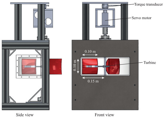
Figure 1.
Schematic view of the turbine system.
The rotation of the turbine was precisely controlled by a servo motor (AKM11B-ANCNC-00) connected to a turbine shaft with a 4.8:1 gear box, and torque exerted by the servo motor was measured using a torque transducer for 5 min at a sampling rate of 100 Hz for each operating condition. Experiments were performed at different angular velocity under the same incoming flow velocity (), to cover a range of tip speed ratios () wide enough to define the performance curve and the turbine optimal conditions, where is defined as the incoming velocity at the blade center ( and ). For each experimental run, the turbine was forced to operate at a constant angular velocity, while the torque was fluctuating due to the incoming turbulence and the turbine rotation. Earlier experiments in vertical axis wind turbine reported that flow-driven and motor-driven turbines show nearly identical wake characteristics and power performances [29,30]. Each blade had an area of 0.10 m by 0.10 m, the radius of the turbine rotation was 0.15 m, and the center of the turbine blade was located at 0.15 m above the bed surface, thus approximately mid-depth. A slight eccentricity of 0.04m, marking the distance between the sidewall and the axis of rotation, is imposed to make sure the shaft and the power conversion systems would be protected within the bank.
Three-dimensional velocity components were measured by side looking Nortek Vectrino+, ADV at a sampling rate of 200 Hz. The velocity measurement locations are shown in Figure 2. Incoming flow velocity was measured at and wake velocity measurements were conducted in a range of () and () at two vertical locations () and (), where x, y, and z are the streamwise, transverse, and vertical coordinates, respectively. The water surface was measured by a Massa M5000 ultrasonic distance sensor, whereas bed elevations were monitored by a submerged sonar device. All the experiment equipment was mounted on a cart that is controlled by a computer: this enabled automatic data acquisition, in particular, moving in the spanwise direction to obtain flow measurements in the lateral boundary layer, and moving in the streamwise direction to assess flow depth invariance and uniform flow conditions.

Figure 2.
(a) The tested prototype turbine model, (b) view of the channel cross section, and (c) planar and (d) lateral side views of the test section with marked measurement locations; x, y, and z are the streamwise, transverse, and vertical coordinates, respectively, corresponding to the velocity components U, V, and W.
The measured raw velocity signals were filtered using a modified phase space threshold (mPST) method [31]. The mPST method eliminates the noise in the signal, generating a three-dimensional threshold ellipsoid in the domain of the signals and their first and second derivative (e.g., U, , and ), respectively. Figure 3a–d shows the streamwise velocity time series before and after the mPST filter at selected locations along the lateral wall (). As reported in earlier research works [31,32,33], the velocity measured by ADV is shown to have large intermittent spikes when the turbulent intensity is high (see P2 and P3 signals in Figure 3b,c). The near wake region (P2 and P3) is observed to be highly turbulent due to complex blade-generated flow structures, which are progressively losing their coherence and intensity as they move downstream (see P4 signal in Figure 3d), resulting in a reduced intermittent spiky velocity signal.
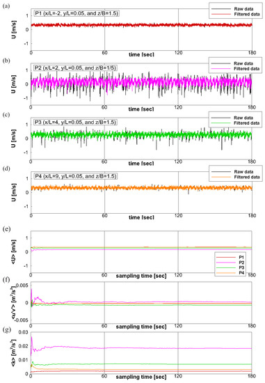
Figure 3.
(a–d) Streamwise velocity time series before and after the postprocessing of the velocity measurements. Temporal convergence study: (e) the streamwise velocity, (f) the primary Reynolds shear stress, and (g) the turbulence kinetic energy averaged over progressively increasing sampling times. P1, P2, P3, and P4 are defined by , and 9 at invariant (nearest point to the lateral side wall) and (at the turbine center height).
Figure 3e–g shows the temporal convergence plots for the streamwise velocity (U), the primary Reynolds shear stress (), and turbulence kinetic energy (), over different averaging time. Herein, represents a time-averaging operator. These graphs show how long it takes for the time-averaged turbulence characteristics to be independent of the sampling time. As seen, the first- and second-order turbulence statistics are converged approximately after 2 min, meaning that most of the turbulent scales that contribute to the energy production can be captured within this period. Accordingly, the velocity was measured over 3 min for all experimental and turbine operating conditions.
3. Results
Prior to investigating the turbine performance and wake flow statistics, we focus on the incoming flow velocity characteristics, in particular on the characterization of the incoming flow within the side wall turbulent boundary layer. Flow measurements were collected upstream of the device at , and are plotted in Figure 4. Shear velocity, (), was estimated by extrapolating the primary Reynolds shear stress () in the proximity of the lateral wall ( and ) to obtain the wall shear stress () on the lateral wall at the vertical location of . As shown in a spanwise profile of the streamwise velocity, fitted by the log-law (Figure 4d), the value of the roughness coefficient (C) in this experiment is somewhat larger than the standard smooth wall values (). This indicates that the wall installed at the right side of the channel is hydrodynamically rough.
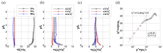
Figure 4.
Incoming flow statistics along the spanwise direction at : (a) mean velocity, (b) Reynolds normal stresses, (c) Reynolds shear stresses, and (d) log-law parametrization of the lateral boundary layer.
3.1. Turbine Performance
One of the advantages of this vertical axis turbine is that the power coefficient can be simply modeled using the momentum balance equation. Power performance for our turbine can be estimated based on the momentum equation, with three model assumptions: (1) the turbine blades outside of the housing structure are only able to absorb the flow momentum, whereas the turbine blades inside the housing structure experience the drag force that counteracts the torque generation. Because the water inside the housing structure is considered in a stationary state, the drag force is exerted on the backside of the blade proportionally to the rotating blade velocity squared of the turbine blade centroid. (2) The radial distance from the origin of rotation, where the flow momentum acts on the front side of the blade, aligns with the location where the drag force acts on the backside of the blade. (3) The flow momentum fluxes bypassing the turbine blades are neglected, so it is assumed that the momentum flux component normal to the blade surface is entirely absorbed by the blade, which leads to an overestimation of the turbine performance by this simplified model. Figure 5 shows details of parameters used in this performance estimation model and the procedure calculating the power performance is described as followed.
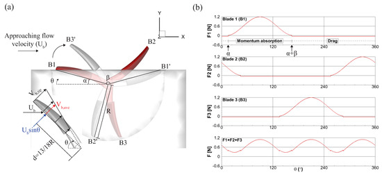
Figure 5.
(a) Schematic view of power coefficient estimation model and (b) expected drag force (F) at the optimal tip speed ratio (), estimated by the forces on the three blades ().
- (i)
- The averaged blade velocity is estimated as
- (ii)
- The flow momentum and drag force exerting on the first blade () is calculated as a function of the phase angle ; the forces on the second () and the third blade () were obtained shifting by and , and , respectively. Here , assuming the backside of the turbine blade resembles a flat plate [34], and are calculated based on the geometry of the turbine system. The resulting force on the first blade is
- (iii)
- To find the point of application of the forces on the blade d, the moment M, resulting from the drag in the cavity, is defined as a function of the radial distance r and compared to the averaged moment :yielding .
- (iv)
- The torque exerting on each blade is then computed asresulting in the net torque as
- (v)
- Eventually, the power coefficient iswhere and are angular velocity and water density, respectively.
Measured and calculated power coefficient curves are plotted in Figure 6. As reported in previous experiments on a lift force-driven vertical axis hydrokinetic turbine, there were uncertainties in obtaining torque values because the generated torque in the turbine model was in the proximity of the lower limit of the measurement range for the torque transducer [25], requiring additional gears. Small sediment particles and organic material present in the Mississippi River water also added uncertainties, as they intermittently induced variability in mechanical friction of the bearing system. Therefore, the ensemble average of the repeated torque measurement for 5 times (solid line) and their minimum and maximum range (dashed line) are presented. Torque measurements were carried out at two different incoming velocity conditions. The first mean flow velocity was chosen to be near the critical mobility condition ( [m/s]), whereas the second mean flow velocity was set slightly higher ( [m/s]), to check the power performance at different Reynolds number. In the case of [m/s], formation of bedforms was avoided. As shown in Figure 6, turbine performances at the two flow conditions collapse within the range of uncertainties, which indicates that the incoming flow conditions have negligible effects on turbine performance, implying that a weak bedload transport beyond critical mobility condition, along with an increase in Reynolds number, have no impact on the power coefficient. The optimal operating condition was found to be at having a range of in the case of [m/s]. The power coefficient is slightly lower as compared to the values of the Savonius wind turbines, ranging from 0.14 to 0.32 (see the work by the authors of [35] and references therein). Note that the simplified power coefficient model overestimates the turbine performance, presenting the maximum of 0.17 at . As mentioned earlier, this overestimation of the analytical model for the maximum power coefficient occurs because we prevent the incoming flow to bypass (or be deflected by) the blade during the time it is exposed to the flow, thus overestimating the absorbed flow momentum. Moreover, the power coefficient curves start showing negative values around when the torque induced by the drag forces in the cavity exceeds the torque generated by the incoming flow momentum on the blades exposed to the flow in the channel.
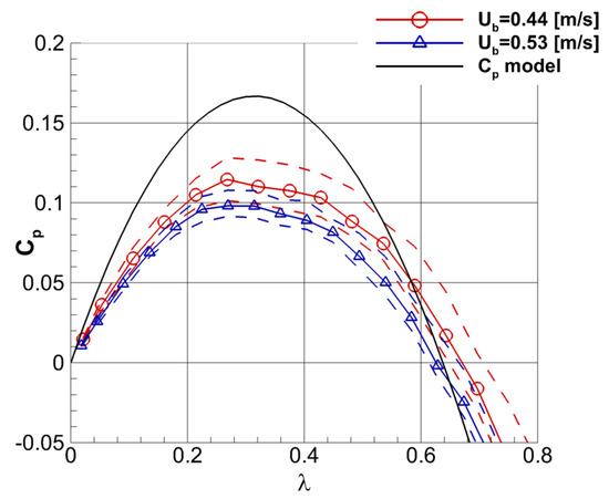
Figure 6.
Power coefficient () curves at two incoming velocities superimposed with result of power coefficient estimation model, where dashed lines represent the minimum and maximum power performance.
3.2. Mean Wake Characteristics
To qualitatively describe the wake characteristics, three-dimensional flow structures downstream of the turbine were schematized in Figure 7. The existence of those flow patterns was inferred based on our experimental results and confirmed with the help of numerical simulations (not shown here as part of future work devoted to optimize the rotor design), using Large Eddy Simulation [36,37]. In the wake of the turbine, the flow is governed by a shear layer, a pair of flow structures rotating in opposite direction with the x-axis, and periodic flows shed by the rotating blades. Wake velocity measurements are analyzed to identify the signature of those blade-generated flow structures.
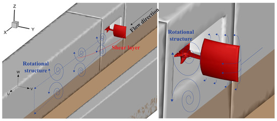
Figure 7.
Schematic view of 3D flow structure observed in the wake of the turbine.
Figure 8 and Figure 9 show contours of mean flow and turbulence characteristics on horizontal plane (x-y plane) at and , respectively, where is the location of the turbine blade center height and is the midpoint between the bottom edge of the turbine blade and channel bed. Herein, represents a time-averaging operator and indicates fluctuating components.
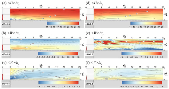
Figure 8.
Dimensionless mean flow velocity contours at (blade center height (a–c) and (the midpoint between the bottom edge of the blade and the channel bed (d–f)).
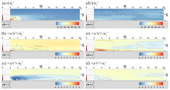
Figure 9.
Dimensionless turbulence characteristics contours at (blade center height, (a–c)) and (the midpoint between the bottom edge of the blade and the channel bed, (d–f)).
Figure 8a shows the streamwise velocity contours, revealing a slow flow region behind the turbine in a range of at . A similar flow pattern is also typically observed in the wake of hydraulic structures installed at a river bank. For instance, in the wake of a cuboid shaped spur dike structure attached to a side wall, a velocity deficit region was observed to form due to flow separation mechanisms [38]. The river bank is protected by the spur dike within this flow region because the velocity gradient and turbulence intensity decrease. The decreased velocity gradient observed in the turbine wake could thus be inferred as a potential benefit for river bank protection. However, wall turbulence structures in the wake of the spur dike and our turbine are found to be significantly different. As shown in Figure 9a, a large amount of the turbulence kinetic energy is generated in the turbine wake at . It is found that periodic momentum flux passing through the turbine blade cross section is responsible for the increase of the turbulence kinetic energy and Reynolds stresses as compared to the spur dike, and will be discussed in more details in the wake dynamics section. It is also important to note that the streamwise velocity contours at and show different flow patterns. The flow is entrained toward the right side of the channel at (Figure 8a), whereas the flow expands toward the left side of the channel at (Figure 8d). This can be explained by flow structures rotating in the opposite direction with the x-axis in the wake of the turbine as sketched in Figure 7.
Figure 8b,e shows the vertical velocity contours. A pair of vortical flow structures is recognized. At (Figure 8b), upward and downward motions are identified in the vertical plane, near the side wall and in the plane close to the exposed blade tip, respectively, suggesting that the flow rotates in the counter-clockwise direction (when looking downstream). On the other hand, downward and upward motions are observed along the side wall and along the exposed tip at (Figure 8e), suggesting the flow rotates in the clock-wise direction. These two signatures suggest the existence of a counter-rotating vortex pair. As drawn in Figure 7, a pair of rotational structures develop due to the different direction of flow entrainment around the turbine blades, sustained by higher velocity bypassing the side edge of the blade as compared to the flow over the top and bottom edges of the blade. These rotational structures, as they are advected downstream, are found to expand in the radial direction, i.e., the outward-facing direction from the axis of the rotational structures (x axis) in the cross-section plane (y-z plane). A footprint of this expansion is plotted in Figure 9e, showing the Reynolds shear stress contours of . The direction of is inferred to determine the sign of : at , is dominant, which implies that the flow structures are likely to move downwards along the vertical direction, contributing to the enhancement of wake recovery [39]. The layer of streamwise velocity at (Figure 8d) expands toward the left side of the channel (when looking downstream), as faster wake recovery occurs due to the vertical advection from the expanding rotational structures.
Another interesting finding is that the primary Reynolds shear stress () is strongly enhanced up to at near the lateral wall (), as shown in Figure 9c. This high region is caused by interactions between the flow entrainment around the blades and the pulsating flows associated with the blade passing frequency, which will be covered in wake dynamics section. The effects of the interaction are observed to be reduced after , where recovers to the incoming flow values defined by the shear velocity at the lateral wall ().
3.3. Wake Dynamics
Periodic motions in the wake of the turbine and their relationships with the mean wake structures are discussed in this section. Power spectra density () function is obtained by calculating the Fourier transform pair of the autocorrelation function of the fluctuating velocity components. Premultiplied spectra () is used to detect the dominant frequency responsible for a large amount of turbulence kinetic energy production, and track its decay along the x direction. Figure 10 shows the premultiplied spectra of u-velocity, where is the blade passing frequency that corresponds to the rotational speed of the turbine shaft [rev/s] multiplied by the number of blades. An intriguing finding is that peaks at the blade passing frequency are detected up to = 7–9. at the blade center height in this experiment (Figure 10a,b). The result is somewhat different from earlier experiment studying a lift force-driven vertical axis turbine. Ouro et al. [22] conducted experiments with three-bladed Gorlov-type vertical axis hydrokinetic turbine and measured velocity in the wake of the turbine using ADV. They reported that peaks at the blade passing frequency are only observed upto (within near-wake), where D is the diameter of the turbine rotor, and the peaks are induced by the dynamic stall vortices emitting from blades. The discrepancy implies that tip vortices shed by blades are not the only factor causing the energy peaks of the streamwise velocity in this experiment. Unlike a lift force-driven vertical axis turbine, the turbine introduced here has more significant periodic blocking effects by blades. The blocking effects deflect the incoming flow momentum and induce a velocity deficit region downstream of the exposed blades when (Figure 5), whereas high momentum flow can freely pass when (Figure 5). This generates seemingly pulsating flows in the wake of the turbine, whose frequency is the same as the blade passing frequency . Note that the energy peaks, despite the small values, persist further downstream at (Figure 10d), as compared to the ones at (Figure 10b) for . It suggests that the pulsating flows advecting the pair of rotating structures discussed above, also affect the unsteadiness of the wake and significantly contribute to the enhancement of the Reynolds stresses.
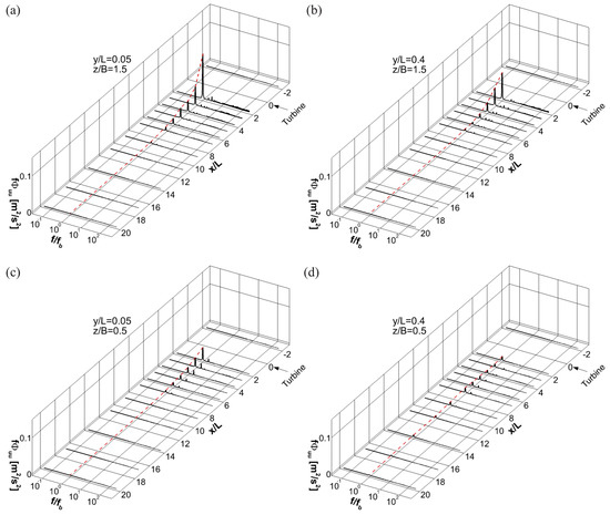
Figure 10.
Premultiplied spectra of the u component (a) near the lateral wall and (b) the blade center at (the blade center height) and (c) near the lateral wall and (d) the blade center at (the midpoint between the bottom edge of the blade and the channel bed).
To deeply understand the effects of the pulsating flows on the wake turbulence, the triple decomposition suggested by Hussain et al. [40] was applied to the measured streamwise velocity signal. The triple decomposition is a mathematical tool that separates time-averaged (), pulsating (), and fluctuating () velocity components from the velocity signal (). Each components in the triple decomposition are calculated as follows. Equation (6), Equations (7)–(9), and Equation (10) describe how to estimate the time-averaged, pulsating (or wave), fluctuating velocity components, respectively.
where is the measured time, is a phase averaging operator, P is the period of the pulsating flows, and is the number of periodicity. Figure 11 shows the triple decomposition at the selected location where the highest premultiplied velocity spectra were observed in Figure 10 (, , and ).
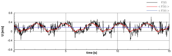
Figure 11.
An example of the triple decomposition: the streamwise velocity signal (black), phase-averaged velocity (red), and time-averaged velocity (blue).
The primary Reynolds shear stress profiles at the lateral wall along the streamwise direction, based on the triple decomposition () and the Reynolds decomposition (), were compared to investigate the effects of periodic pulsating flow characteristics on the lateral wall shear stress. The estimation of the wall shear stress in unsteady flows (e.g., in vegetated channel flows, where periodically shedding vortex streaks) using measured velocity needs some extra caution because most wall shear stress prediction methods in the literature were derived and tested for straight channels with distributed roughness [41]. Duan et al. [42] reported that bed shear stress distributions estimated by the Reynolds shear stresses were able to predict a scour region in the wake of a spur dike in erodible beds (where no logarithmic law parametrization could be assessed). Therefore, we infer that the primary Reynolds shear stress () can be used here to quantify the lateral wall shear stress. Other Reynolds shear stress components ( and ) are ignored as the values are small compared to the primary Reynolds shear stress.
Figure 12 plots the longitudinal distributions of the primary Reynolds shear stress at the closest measurement points to the lateral wall () at the turbine blade center height (). Deviation of instantaneous velocity from the time-averaged velocity in the Reynolds decomposition consists of the pulsating and fluctuating components of the triple decomposition (). Therefore, the primary Reynolds shear stress, based on the Reynolds decomposition, is expressed with four terms of velocity components in the triple decomposition (). Contribution of each term to , which indicates the strength of lateral wall shear stress, is analyzed in Figure 12. These graphs are normalized by at (). Since the pulsating flows originate from periodically passing momentum flux through the blades in the wake of the turbine, there is no discrepancy between and in an upstream region of the turbine. As shown in Figure 12, is observed to be the greatest contributor to the increase of . This means that pulsating flows significantly increase the unsteadiness of the flow near the lateral wall, and we expect this to induce high lateral wall shear stress. On the other hand, cross-correlated terms in the triple decomposition ( and ) were observed to have negligible effects on by compensating with each other.
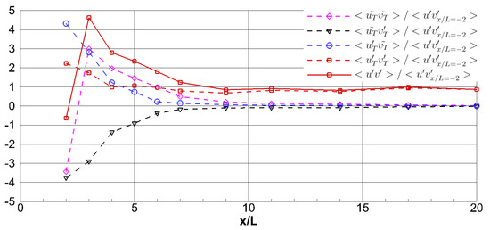
Figure 12.
Normalized longitudinal distributions of the primary Reynolds shear stress near the lateral wall () at the turbine blade center height () based on the triple (dashed lines) and Reynolds decompositions (solid line).
Figure 12 shows that reaches its undisturbed state () at , and it is reduced to 67% compared to its upstream value in a range = 6–11. Moreover, the profiles of and are observed to collapse into one graph after , which implies that pulsating flow characteristics disappear. This explains why the high energy peaks in the streamwise velocity spectra are detected upto in Figure 10a. It is also important to note that the increase of is observed in the near wake (upto ). Three-dimensional flow structures, such as tip vortices and vortex shedding, are assumed to be responsible for this increase.
4. Discussion
The experimental results showed that periodic pulsating momentum flux amplifies the unsteadiness of the flow in the wake of the turbine. Although this unsteady turbulent flow is likely to increase the erodibility of a river bank in a straight channel, as suggested in this experiment, the relation between unsteady turbulent flows and bank stability in a meandering channel remains unclear. The turbine we introduce in this paper is designed to be installed in a meandering river where more energetic flows are observed in the outer bank, to maximize the hydrokinetic energy. It was reported that the secondary flow is a crucial driving agent responsible for the bank erosion, transporting sediment from the stream bank to the channel center [43]. In our experiments, it is observed that the turbine creates a marked velocity deficit region in the near-wake (Figure 8a). The secondary flow in meandering rivers is known to be generated by the centrifugal force originating from nonuniformly distributed velocity field in the cross section characterized by higher velocity and surface elevation along the outer bank. The velocity deficit region, potentially extended by multiple deployed turbines, is expected to counteract the high velocity region characteristic of undisturbed outer banks, and thus is likely to mitigate the sustainment of the secondary flow. We speculate that our vertical axis turbine might reduce the secondary flow contribution to bank erosion in meandering rivers. The experiment results showed that the time-averaged streamwise velocity in the wake of our vertical axis hydrokinetic turbine have similar flow patterns as those observed in the wakes of hydraulic structures used for bank protection (e.g., spur dike, vane, etc.). In particular, the streamwise velocity gradient in the wake was reduced, suggesting possible mitigation of river bank erosion.
However, it is still necessary to reduce the unsteadiness of the wake flow to dampen the Reynolds stress contribution near the lateral wall, which works against bank stability. One plausible solution might be adding a deflector in the wake region, expanding from the lateral wall. Because the streamwise velocity is reduced in the wake and the periodic pulsating flows passing around turbine blades are responsible for the added vorticity near the bank, it is inferred that even small structure extruding from the later wall could deflect the blade generated flow structures towards the channel center and avoid the increase in Reynolds stresses along the sidewall.
5. Conclusions
A new installation concept for a drag-driven vertical axis hydrokinetic turbine is introduced in this study and supported by performance quantification and wake characterization. Although the design of the turbine rotor is not novel, same working principle as a Savonius turbine, the deployment strategy is original. The three-bladed turbine system is designed to extract streamwise momentum in shallow waters, and it is particularly suited for the outer banks of meandering rivers. The turbine system is partially embedded in the stream bank to favor torque generation, to shelter the turbine shaft, and to keep the in-line sensors and power electronics out of the water, thus reducing operation and maintenance costs. Flume experiments were conducted to test a reduced-scale model in a straight open channel flow using ADV and a controlled motor drive coupled with torque transducer. Power performance was measured, and modeled, simply, for varying tip speed ratios at two flow discharges, characterized by critical mobility and low bedload transport, respectively. The results showed that the power coefficient curves are fairly independent of the Reynolds number suggesting that performance can be scaled up in physical or numerical investigation at the prototype scale. Time-averaged wake velocity deficit and unsteady flow structures shed by the turbine are investigated up to and will be used to validate numerical simulations. Two rotating structures, carrying the spectral signature of the blade passing frequency, are consistently observed in the wake of the turbine and are considered as a major source of unsteadiness in the wake. Their strong contribution to the Reynolds stresses at the side wall is expected to reduce bank stability in the straight channel configuration so far investigated. However, it was observed that the streamwise velocity, along the cross flow direction, is significantly reduced in the wake, which could have some implications for the evolution of meandering flows. The potential interaction between the turbine wake structures, its velocity deficit region, and the secondary current along the outer banks of meandering channels must be investigated and quantified. If this turbine system can disrupt or mitigate the formation of the secondary flow in meandering rivers, which is the main driving factor for river bank erosion, its value and applicability would be significantly increased. Further numerical and experimental studies will be conducted aiming at design optimization of the turbine rotor and quantification of the interaction with secondary currents in meandering flows. The primary goal is to improve momentum absorbtion, possibly varying the curvature of the blade, so as to improve the performance and reduce the intensity of the unsteady large scale structures in the near-wake of the turbine (eventually reducing stream bank shear stress). For instance, the power performance of this preliminary design can be enhanced by increasing the inner surface blade curvature. In this study, the blade drag coefficient is simply assumed as a flat plate () due to its mild curvature; however, it can be increased up to , assuming the blades have an hemispherical shape [34]. It is also important to note that the drag forces exerting on the back side of the turbine blades, which counteracts the torque generation, can be reduced by increasing the outer surface blade curvature, also leading to potential improvement of the turbine performance. Therefore, a different blade design could allow the turbine to absorb more kinetic energy and momentum entailed in the flows. Other relevant design goals are (i) deflecting blade generated structures from the side bank to the channel center, to reduce Reynolds stresses at the stream bank, and (ii) optimizing deployment strategy in a meandering river, with multiple spaced and/or vertically staggered devices.
6. Patents
The intellectual property is currently protected under US Patent App. 15/914,183 (pending) filed through the University of Minnesota Office of Technology and Commercialization (OTC).
Author Contributions
J.L. conducted the experiments, performed data analysis, and wrote a significant portion of the manuscript; M.M. contributed to the design and testing of the turbine and defined the channel hydraulic conditions and acquisition system; C.F. built the turbine model; and J.G. and L.S. conducted a comparison simulation study, participated in the discussion of the experiment results, and contributed to the writing of the manuscript. M.G. envisioned the turbine, provided financial support, and planned experiments and measuring strategy. Conceptualization, M.M., L.S. and M.G.; Data curation, J.L. and M.G.; Formal analysis, J.L., M.M. and M.G.; Funding acquisition, L.S. and M.G.; Investigation, J.L., M.M., C.F., J.G., L.S. and M.G.; Methodology, J.L., M.M., C.F., L.S. and M.G.; Project administration, L.S. and M.G.; Resources, C.F.; Supervision, L.S. and M.G.; Validation, J.L., M.M., C.F., J.G., L.S. and M.G.; Visualization, J.L., J.G., L.S. and M.G.; Writing—original draft, J.L. and M.G.; Writing—review and editing, J.L., M.M., J.G., L.S. and M.G.
Funding
This research was funded by the Institute on the Environment (IonE) at the University of Minnesota (Grant No. DG-0003-16).
Conflicts of Interest
The authors declare no conflict of interest.
Nomenclature
| Q | Volume flow rate [m/s] |
| D | Rotor diameter [m] |
| Median grain size [mm] | |
| W | Channel width [m] |
| h | Water depth [m] |
| Turbine center height [m] | |
| R | Radius of turbine rotation [m] |
| L | Turbine blade length extruding from the channel sidewall [m] |
| B | Vertical width of turbine blade [m] |
| d | Point of application of forces on the blade [m] |
| r | Radial distance from the origin of turbine rotation [m] |
| Streamwise, transverse, and vertical coordinates [m] | |
| A | Turbine blade area [m] |
| Cross sectional velocity [m/s] | |
| Blade center velocity [m/s] | |
| Blade tip velocity [m/s] | |
| Averaged blade velocity [m/s] | |
| Shear velocity at the channel sidewall [m/s] | |
| Fluctuating velocity components in the Reynolds decomposition in x, y, and z direction [m/s] | |
| Fluctuating velocity components in the triple decomposition in x, y, and z direction [m/s] | |
| Pulsating velocity components in the triple decomposition in x, y, and z direction [m/s] | |
| k | Turbulence kinetic energy [m/s] |
| g | Gravity [m/s] |
| Kinematic viscosity [m/s] | |
| Water density [kg/m] | |
| Bed shear stress [kg/(ms)] | |
| M | Moment [kg(m/s)] |
| Turbine blades | |
| Forces exerted on each blade | |
| Net torque and torque generated at each blade [kg(m/s)] | |
| Power spectra density [m/s] | |
| Frequency and the blade passing frequency [1/s] | |
| Angular velocity [1/s] | |
| Measurement time [s] | |
| Water slope [%] | |
| Angle where active phase starts and ends [] | |
| Angular location [] | |
| Temperature [C] | |
| Standard deviation of temperature [C] | |
| Tip speed ratio | |
| Power coefficient | |
| Drag coefficient | |
| Reynolds number based on water depth | |
| Reynolds number based on turbine rotor diameter | |
| Reynolds number based on blade chord length | |
| Froude number | |
| C | Hydraulic roughness coefficient |
| Time-averaging operator | |
| Phase averaging operator | |
| P | Period of the pulsating flows |
| N | Number of periodicity |
References
- Bahaj, A.; Molland, A.; Chaplin, J.; Batten, W. Power and thrust measurements of marine current turbines under various hydrodynamic flow conditions in a cavitation tunnel and a towing tank. Renew. Energy 2007, 32, 407–426. [Google Scholar] [CrossRef]
- Maganga, F.; Germain, G.; King, J.; Pinon, G.; Rivoalen, E. Experimental characterisation of flow effects on marine current turbine behaviour and on its wake properties. IET Renew. Power Gener. 2010, 4, 498–509. [Google Scholar] [CrossRef]
- Kang, S.; Borazjani, I.; Colby, J.A.; Sotiropoulos, F. Numerical simulation of 3D flow past a real-life marine hydrokinetic turbine. Adv. Water Resour. 2012, 39, 33–43. [Google Scholar] [CrossRef]
- Chamorro, L.; Hill, C.; Morton, S.; Ellis, C.; Arndt, R.; Sotiropoulos, F. On the interaction between a turbulent open channel flow and an axial-flow turbine. J. Fluid Mech. 2013, 716, 658–670. [Google Scholar] [CrossRef]
- Chamorro, L.P.; Troolin, D.R.; Lee, S.J.; Arndt, R.; Sotiropoulos, F. Three-dimensional flow visualization in the wake of a miniature axial-flow hydrokinetic turbine. Exp. Fluids 2013, 54, 1459. [Google Scholar] [CrossRef]
- Kang, S.; Yang, X.; Sotiropoulos, F. On the onset of wake meandering for an axial flow turbine in a turbulent open channel flow. J. Fluid Mech. 2014, 744, 376–403. [Google Scholar] [CrossRef]
- Okulov, V.L.; Naumov, I.V.; Mikkelsen, R.F.; Kabardin, I.K.; Sørensen, J.N. A regular Strouhal number for large-scale instability in the far wake of a rotor. J. Fluid Mech. 2014, 747, 369–380. [Google Scholar] [CrossRef]
- Ouro, P.; Harrold, M.; Stoesser, T.; Bromley, P. Hydrodynamic loadings on a horizontal axis tidal turbine prototype. J. Fluids Struct. 2017, 71, 78–95. [Google Scholar] [CrossRef]
- Mycek, P.; Gaurier, B.; Germain, G.; Pinon, G.; Rivoalen, E. Experimental study of the turbulence intensity effects on marine current turbines behaviour. Part I: One single turbine. Renew. Energy 2014, 66, 729–746. [Google Scholar] [CrossRef]
- Chamorro, L.; Hill, C.; Neary, V.; Gunawan, B.; Arndt, R.; Sotiropoulos, F. Effects of energetic coherent motions on the power and wake of an axial-flow turbine. Phys. Fluids 2015, 27, 055104. [Google Scholar] [CrossRef]
- Blackmore, T.; Myers, L.E.; Bahaj, A.S. Effects of turbulence on tidal turbines: Implications to performance, blade loads, and condition monitoring. Int. J. Mar. Energy 2016, 14, 1–26. [Google Scholar] [CrossRef]
- Hill, C.; Musa, M.; Chamorro, L.P.; Ellis, C.; Guala, M. Local scour around a model hydrokinetic turbine in an erodible channel. J. Hydraul. Eng. 2014, 140, 04014037. [Google Scholar] [CrossRef]
- Hill, C.; Kozarek, J.; Sotiropoulos, F.; Guala, M. Hydrodynamics and sediment transport in a meandering channel with a model axial-flow hydrokinetic turbine. Water Resour. Res. 2016, 52, 860–879. [Google Scholar] [CrossRef]
- Hill, C.; Musa, M.; Guala, M. Interaction between instream axial flow hydrokinetic turbines and uni-directional flow bedforms. Renew. Energy 2016, 86, 409–421. [Google Scholar] [CrossRef]
- Musa, M.; Heisel, M.; Guala, M. Predictive model for local scour downstream of hydrokinetic turbines in erodible channels. Phys. Rev. Fluids 2018, 3, 024606. [Google Scholar] [CrossRef]
- Mycek, P.; Gaurier, B.; Germain, G.; Pinon, G.; Rivoalen, E. Experimental study of the turbulence intensity effects on marine current turbines behaviour. Part II: Two interacting turbines. Renew. Energy 2014, 68, 876–892. [Google Scholar] [CrossRef]
- Chawdhary, S.; Hill, C.; Yang, X.; Guala, M.; Corren, D.; Colby, J.; Sotiropoulos, F. Wake characteristics of a TriFrame of axial-flow hydrokinetic turbines. Renew. Energy 2017, 109, 332–345. [Google Scholar] [CrossRef]
- Musa, M.; Hill, C.; Sotiropoulos, F.; Guala, M. Performance and resilience of hydrokinetic turbine arrays under large migrating fluvial bedforms. Nat. Energy 2018, 3, 839. [Google Scholar] [CrossRef]
- Musa, M.; Hill, C.; Guala, M. Interaction between hydrokinetic turbine wakes and sediment dynamics: Array performance and geomorphic effects under different siting strategies and sediment transport conditions. Renew. Energy 2019, 138, 738–753. [Google Scholar] [CrossRef]
- Dabiri, J.O. Potential order-of-magnitude enhancement of wind farm power density via counter-rotating vertical-axis wind turbine arrays. J. Renew. Sustain. Energy 2011, 3, 043104. [Google Scholar] [CrossRef]
- Strom, B.; Brunton, S.L.; Polagye, B. Intracycle angular velocity control of cross-flow turbines. Nat. Energy 2017, 2, 17103. [Google Scholar] [CrossRef]
- Ouro, P.; Runge, S.; Luo, Q.; Stoesser, T. Three-dimensionality of the wake recovery behind a vertical axis turbine. Renew. Energy 2019, 133, 1066–1077. [Google Scholar] [CrossRef]
- Li, Y.; Calisal, S.M. Three-dimensional effects and arm effects on modeling a vertical axis tidal current turbine. Renew. Energy 2010, 35, 2325–2334. [Google Scholar] [CrossRef]
- Bachant, P.; Wosnik, M. Performance measurements of cylindrical-and spherical-helical cross-flow marine hydrokinetic turbines, with estimates of exergy efficiency. Renew. Energy 2015, 74, 318–325. [Google Scholar] [CrossRef]
- Bachant, P.; Wosnik, M. Effects of Reynolds number on the energy conversion and near-wake dynamics of a high solidity vertical-axis cross-flow turbine. Energies 2016, 9, 73. [Google Scholar] [CrossRef]
- Yang, B.; Lawn, C. Fluid dynamic performance of a vertical axis turbine for tidal currents. Renew. Energy 2011, 36, 3355–3366. [Google Scholar] [CrossRef]
- Golecha, K.; Eldho, T.; Prabhu, S. Influence of the deflector plate on the performance of modified Savonius water turbine. Appl. Energy 2011, 88, 3207–3217. [Google Scholar] [CrossRef]
- Harries, T.; Kwan, A.; Brammer, J.; Falconer, R. Physical testing of performance characteristics of a novel drag-driven vertical axis tidal stream turbine; with comparisons to a conventional Savonius. Int. J. Mar. Energy 2016, 14, 215–228. [Google Scholar] [CrossRef]
- Araya, D.B.; Dabiri, J.O. A comparison of wake measurements in motor-driven and flow-driven turbine experiments. Exp. Fluids 2015, 56, 150. [Google Scholar] [CrossRef]
- Dou, B.; Guala, M.; Lei, L.; Zeng, P. Experimental investigation of the performance and wake effect of a small-scale wind turbine in a wind tunnel. Energy 2019, 166, 819–833. [Google Scholar] [CrossRef]
- Parsheh, M.; Sotiropoulos, F.; Porté-Agel, F. Estimation of power spectra of acoustic-Doppler velocimetry data contaminated with intermittent spikes. J. Hydraul. Eng. 2010, 136, 368–378. [Google Scholar] [CrossRef]
- Cea, L.; Puertas, J.; Pena, L. Velocity measurements on highly turbulent free surface flow using ADV. Exp. Fluids 2007, 42, 333–348. [Google Scholar] [CrossRef]
- Goring, D.G.; Nikora, V.I. Despiking acoustic Doppler velocimeter data. J. Hydraul. Eng. 2002, 128, 117–126. [Google Scholar] [CrossRef]
- Hoerner, S.F. Fluid Dynamic Drag; Published by the Author: Midland Park, NJ, USA, 1965; pp. 3–19. [Google Scholar]
- Akwa, J.V.; Vielmo, H.A.; Petry, A.P. A review on the performance of Savonius wind turbines. Renew. Sustain. Energy Rev. 2012, 16, 3054–3064. [Google Scholar] [CrossRef]
- He, S.; Yang, Z.; Shen, L. Numerical Simulation of Interactions among Air, Water, and Rigid/Flexible Solid Bodies. In Proceedings of the 10th International Workshop on Ship and Marine Hydrodynamics, Keelung, Taiwan, 5–8 November 2017. [Google Scholar]
- Cui, Z.; Yang, Z.; Shen, L.; Jiang, H. Complex modal analysis of the movements of swimming fish propelled by body and/or caudal fin. Wave Motion 2018, 78, 83–97. [Google Scholar] [CrossRef]
- Jeon, J.; Lee, J.Y.; Kang, S. Experimental Investigation of Three-Dimensional Flow Structure and Turbulent Flow Mechanisms Around a Nonsubmerged Spur Dike With a Low Length-to-Depth Ratio. Water Resour. Res. 2018, 54, 3530–3556. [Google Scholar] [CrossRef]
- Bachant, P.; Wosnik, M. Characterising the near-wake of a cross-flow turbine. J. Turbul. 2015, 16, 392–410. [Google Scholar] [CrossRef]
- Hussain, A.K.M.F.; Reynolds, W.C. The mechanics of an organized wave in turbulent shear flow. J. Fluid Mech. 1970, 41, 241–258. [Google Scholar] [CrossRef]
- Yang, J.Q.; Kerger, F.; Nepf, H.M. Estimation of the bed shear stress in vegetated and bare channels with smooth beds. Water Resour. Res. 2015, 51, 3647–3663. [Google Scholar] [CrossRef]
- Duan, J.G.; He, L.; Fu, X.; Wang, Q. Mean flow and turbulence around experimental spur dike. Adv. Water Resour. 2009, 32, 1717–1725. [Google Scholar] [CrossRef]
- Odgaard, A.J.; Mosconi, C.E. Streambank protection by submerged vanes. J. Hydraul. Eng. 1987, 113, 520–536. [Google Scholar] [CrossRef]
© 2019 by the authors. Licensee MDPI, Basel, Switzerland. This article is an open access article distributed under the terms and conditions of the Creative Commons Attribution (CC BY) license (http://creativecommons.org/licenses/by/4.0/).