Abstract
Tidal energy converter (TEC) arrays in tidal channels generate complex flow phenomena due to interactions with the local environment and among devices. Models with different resolutions are thus employed to study flows past TEC farms, which consider multiple spatial and temporal scales. Simulations over tidal cycles use mesoscale ocean circulation models, incorporating a thrust coefficient to model the momentum sink that represents the effects of the array. In this work, we propose an expression for a thrust coefficient to represent finite-sized farms of TEC turbines at larger scales, , which depends on the spatial organization of the devices. We use a coherent-structure resolving turbulence model coupled with the actuator disk approach to simulate staggered turbine configurations in more detail, varying the separation among devices and the ratios between the channel depths and hub heights. Based on these simulations, we calculate the resultant force for various subsets of devices within the farm, and their corresponding effective thrust coefficient, . We conclude that the thrust coefficient depends solely on the lateral separation of the devices, , for farms with only two rows. For farms with more than two rows, the streamwise distance, , must be considered as well. With the proposed expression, it is possible to calculate efficiently the effects of finite-sized TEC farms and incorporate a momentum sink into ocean circulation models, without assuming a constant coefficient derived from an infinite farm approximation.
1. Introduction
The extraction of kinetic energy from tidal currents using tidal energy converters (TEC) can contribute to solving problems associated with the increase of global energy demand and greenhouse gas emissions [1]. Tidal energy is characterized by being predictable, CO emission-free in operation, with a minimal visual impact. Furthermore, plenty of studies have shown a considerable amount of extractable power from tides available around the world [2,3,4,5]. However, there are just a handful of marine energy projects in construction or testing. Nevertheless, despite the fact that harnessing energy from the tides could potentially be a positive contribution to the energy supply, the impacts on the tidal flow itself are yet unclear; for this reason, it is essential to first analyze and assess the hydrodynamic effects at mesoscales before any installation.
Numerical simulations can provide quantitative information of the interactions between the flow, the turbines, and the environment, to understand the physics at different temporal and spatial scales in the ocean. Their advantage is that they can provide full temporal and spatial data over an entire computational domain. However, it is not possible to use just one type of modeling strategy to understand all relevant scales due to computational cost restrictions. For example, while the interaction between tides and turbine farms can be represented by using mesoscale ocean circulation models, the resolution of these models does not allow for the representation of individual devices and their wakes. As a result, accurate parameterizations are needed. At the same time, the turbine wake and its interaction with other wakes can be accurately represented by high-resolution, turbulence-resolving models that cover smaller temporal and spatial scales. In this way, they are useful for understanding the fundamental physical processes required for upscaling the effects of TEC farms.
To represent multiple TEC devices in ocean circulation models, it is necessary to incorporate a sink of momentum in the section of the domain where the group of turbines will be located. For this, one option is to add to the momentum conservation equation a thrust force applied by a single turbine, multiplied by the number of devices in the grid element. In the literature, we can see how this approach has been used to predict the effect of TEC devices in real tidal channels (e.g., [6,7,8]). However, this strategy does not consider the changes produced on the resistance force caused by different turbine distributions in a farm. Recently, Piano et al. [9] demonstrated that neglecting the interaction between devices is a reasonable approximation for upscaling the effect of farms with less than 25 turbines into two-dimensional vertically-averaged ocean models. However, we cannot assume the same for three-dimensional ocean models, especially for flows with substantial vertical velocity components. Another option for incorporating the effect of turbines into large scale models is to represent just one device per grid cell. In this case, the distribution of the devices will be restricted by the grid resolution, which can represent a problem because depending on the inter-turbine spacing, the velocity of the flow can change in direction and magnitude [10].
Some studies have presented parameterizations for farms of TEC devices. One example is the work of Nishino and Willden [11], which showed the idea of a global thrust coefficient representative of an entire farm. In their work, Nishino and Willden [11] calculated the efficiency of a group of turbines based on the local, and global blockage areas, which are defined as the ratio between the area of the devices over the farm area, and the entire domain area, respectively. Nonetheless, the analytical formulation they proposed is only valid for very large farms. Another study of farms’ parameterization is the one of Stansby and Stallard [12], which represented and optimized arrangements of tidal turbines, by proposing a correction factor to the blockage area that considers the velocity deficit, and the turbines upstream every row. Although the results of [12] have shown good agreement with experimental cases, they did not provide a formula that could be extended for other arrays.
Since many of the physical processes that are observed in the flow past TEC devices are similar to conditions in wind turbines, we can refer to the literature related to wind energy, where there is a wider variety of numerical simulations and field measurements. Fitch et al. [13], for example, proposed and validated a parameterization scheme for a group of wind turbines on a mesoscale atmospheric model. Their representation, however, does not consider the spatial distribution of the devices, and the limitations of the model concerning the separation distance are unclear since they did not study cases where the wakes of the devices have a strong interaction due to their proximity. Later, Abkar and Porté-Agel [14] improved the parameterization of Fitch et al. [13] by using large eddy simulations (LES) to incorporate the effects of the distribution of turbines on the flow. They assumed periodic boundaries, following a common approach in wind turbine simulations (e.g., [15,16,17]), since wind farms are often sufficiently large to allow the flow to reach a fully developed state inside the arrangement. In contrast, the largest TEC farm installed in the world does not exceed five turbines, and an accurate representation of tidal energy farms in larger scale models requires improving our understanding on the interaction of devices in finite domains.
Additional differences arise when comparing wind turbine farms and TEC arrays, such as the vertical position of the devices within the turbulent boundary layer. In the case of wind farms, the atmospheric boundary layer thickness is around 1000 m, and the wakes downstream of the devices are not confined from above. In the case of tidal energy, the free surface of the flow represents a boundary that restricts the development of a symmetrical Gaussian wake and affects the velocity recovery [18]. In some cases, turbines are close to the interface, generating disturbances of the free surface that decrease considerably the performance of the devices [19]. Thus, for farms of TEC turbines, it is necessary to take into account the depth of the devices in addition to their lateral separation.
To study the effects of varying TEC farm configurations, we perform a systematic study by using high-resolution numerical simulations to represent different arrangements of turbines. To simulate the flow around the devices, we utilize the hybrid Detached-Eddy Simulations (DES) turbulence model [20,21,22,23,24], and the TEC devices are represented by the actuator disk approach [25], where a sink of momentum is incorporated at the area occupied by each turbine. From these simulations, we calculate the momentum sink of farms with different distributions, number of devices, and depths. Finally, we introduce a new dimensionless thrust coefficient, , which is meant to represent the entire group of turbines. With the use of , we seek to improve the representation of turbine arrays in ocean circulation models by incorporating the interactions among devices, according to the geometric characteristics of the farm. The improved representation can be used to study the interaction between entire farms of turbines and a real environment by running larger-scale numerical simulations that use data of bathymetry and tidal cycles. Results indicate that, for staggered farms, only depends on the lateral separation of the devices for farms with two rows, and on the lateral and longitudinal separation for farms with more rows. Furthermore, we show that this parameter is independent of the number of columns of devices, as well as the ratio of the depth over the hub height (up to a value of ).
The paper is organized as follows: In Section 2, we describe the numerical method and the validation of the model with experimental results. In Section 3, we formulate the representation of an array of devices by performing an analysis of the flow resistance induced by an array. Finally, in Section 4, we summarize the findings of this investigation and propose topics for future work.
2. Methods
In this section, we introduced and validated the DES model, coupled with the actuator disk approach. Using this combined model in a series of simulations, we proposed a new thrust coefficient, , to represent finite-sized farms of turbines, parameterized by the most relevant physical variables of the flow. Various turbine arrangements were studied to propose a versatile thrust coefficient for representing TEC farms which lie entirely within large-scale circulation model grid cells.
2.1. Numerical Simulations
We employed the DES approach, which is a hybrid one-equation turbulence model that works as a Reynolds averaged Navier–Stokes (RANS) model near the solid boundaries and as LES away from them. The advantages of DES are that it can resolve the large-scale dynamics of turbulence formed in the wakes of the disks by using the LES approach at high Reynolds numbers. Meanwhile, the computational costs are reduced by modeling the turbulent boundary layer with a RANS approach. The governing equations used in DES were the incompressible three-dimensional Reynolds-averaged Navier–Stokes equations for mass and momentum conservation. The non-dimensional equations were written as follows:
where are the Cartesian coordinates () in the streamwise, spanwise, and vertical directions, respectively, is the velocity of the fluid in the direction i, is the pressure, is the Reynolds number based on the length scale, ℓ, and a velocity scale, V, and is the non-dimensional thrust force per unit mass exerted by the turbines. The Reynolds stresses in Equation (2) were modeled by using the Spalart–Allmaras (S–A) turbulence closure, which implements a single transport equation for a term related to the turbulent viscosity, [20]. The turbulent destruction term in this equation is scaled with the distance to the nearest wall, while far from solid boundaries is scaled with the grid size, becoming a subgrid-scale model for LES in regions away from the wall, when the production balances the destruction term. Since it has been shown that the inlet turbulence intensity is important for accurately simulating turbines [26,27], we incorporated into our model an inlet random flow generator, using the formulation proposed in [28]. This is a stochastic approach, where the inlet averaged velocity and fluctuations in time, , can easily be set by using experimental data. We have to highlight that the inputs for this model are a fully developed vertical profile of the streamwise velocity, and a unique value for the components .
In the actuator disk approach, the thrust force per unit mass, per unit of volume, is incorporated in the stream-flow direction (), where:
In Equation (3), is the disk area, is the thrust coefficient of a single turbine, is the differential volume occupied by the turbine in the discretized domain, and is the streamwise undisturbed velocity magnitude upstream of the disk.
In a turbine farm using this common parameterization, it is not always clear what velocity scale can be used to replace the undisturbed velocity, . For that reason, a second parameterization can be defined based on the the local velocity at the disk, , instead of using to calculate the force exerted by the device. To implement this, we used a modified thrust coefficient , which is related to as follows:
where a is a so-called induction factor [25]. In this way, we calculated the thrust force by using the following expression, which is equivalent to Equation (3), but it is now based on the local flow velocity seen by the disk:
Model Validation
For validating the DES coupled with the actuator disk approach, we replicated the laboratory experiments of Chamorro and Porté-Agel [29], and, later, by Markfort et al. [30]. The experimental configuration consists of 30 scaled turbines distributed in a staggered way along a wind tunnel; this is shown in the schematic of Figure 1. In the experiments, the velocity and turbulence up- and downstream of the turbines were measured by using a hot-wire anemometer. In the wind tunnel, the Reynolds number based on the freestream velocity at the hub height, , was equal to 36,000. In our simulations, we used the same averaged inlet velocity and turbulence intensity profiles as measured in the wind tunnel. Regarding the lateral walls, we used a symmetric boundary condition.
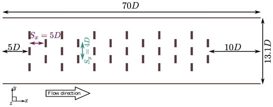
Figure 1.
Schematic distribution of disks for the validation of numerical simulations, following the laboratory experiments of Chamorro and Porté-Agel [29] and Markfort et al. [30].
To represent the disks, we distribute the thrust coefficient, , along the area covered by the devices by using a Gaussian distribution with an average , and a standard deviation, , where D is the disk diameter. The computational domain is discretized using million nodes, which allows each disk to contain at least seven grid points in the vertical direction and five in the spanwise direction, as suggested in the literature [31].
To make a quantitative comparison between the results of our simulations and the experimental data, we utilized the root mean square error ()-observations standard deviation ratio () [32], which is defined for any variable as:
where n is the total number of records, are the observed data, are the simulated results in the same location that observed data, and is the average of the observed values. The fluctuates from zero for optimal conditions, to a large positive value.
From the results of the numerical simulations, we calculated the time-averaged velocity and turbulence intensity profiles in the streamwise direction to compare them with measurements of Markfort et al. [30] taken three diameters downstream the 1st, 5th, and 11th rows of turbines. On one hand, the mean velocity profiles showed good agreement with the measured data (see Figure 2), and, for all the cases, the calculated did not exceed . The turbulence intensity profiles exhibited more disagreement, particularly downstream of the first row of turbines. Downstream of the 5th and the 11th rows, however, our model performs better (see Figure 3), with an close to 2. The simulations captured the vertical distribution, resolving almost the entire measured turbulence intensity. It is important to note that the measurements reported the total turbulent intensity, whereas the computed values corresponded only to the resolved component, since the Spalart–Allmaras model could not readily yield the modeled component of the normal stresses. The largest differences in the turbulence of the wake for the first row were produced by the influence of the turbine geometry compared to the disk simplification, and the results for this statistic improve considerably downstream as shown in Figure 3.
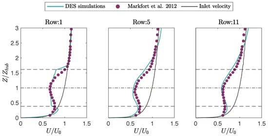
Figure 2.
Mean streamwise velocity normalized by (the inlet velocity at the hub height, ) as a function of , downstream of the 1st, 5th, and 11th rows of turbines. Circles show measurements (Data from: Markfort et al. [30]). Continuous lines are the results from the DES simulations coupled with the actuator disk approach. Dashed lines mark the bottom, center, and top of the disks.
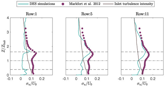
Figure 3.
Turbulence intensity in the streamwise direction () profile as a function of , downstream of the 1st, 5th, and 11th rows of turbines. Circles show measurements (Data from: Markfort et al. [30]). Continuous lines are the results from the DES simulations coupled with the actuator disk approach. Dashed lines mark the bottom, center, and top of the disks.
We have to highlight that, even though these experiments were carried out in a wind tunnel, the results are equally valid for tidal applications. The last is true because the model does not distinguish the kind of fluid, but it uses the Reynolds number as input, which is in a turbulent range. The choice of this experimental case to validate our model was motivated by the large number of devices it presents, and the available measured data. Furthermore, we have to mention that Gajardo et al. [24] validated the DES model coupled with a more complex turbine representation, known as Blade Element Momentum, by replicating the flume experiments of the PerAWaT project carried out by Stallard et al. [33].
2.2. Parameterization of Farms of TEC Devices
In this section, we calculate the resultant force exerted by a finite-sized farm and the corresponding thrust coefficient from the DES results. We then discuss the main parameters that should be considered for representing turbine arrays in larger scale models. Finally, we present the simulations used to study how the thrust coefficient of a farm changes with the internal distribution of the disks.
2.2.1. Resultant Force for a Turbine Farm
The resultant force exerted by different turbine arrays is calculated by using the simulated data of the validation case. To do this, we computed the net flux of momentum in the streamwise direction for several control volumes, considering the pressure drop and the viscous losses. These control volumes consider the total height of the channel, and enclose different numbers of rows, as is shown in the schematic of Figure 4. We emphasize that, in this case, we could isolate different control volumes inside the farms to calculate , rather than running entirely independent calculations. For example, when we run a case with exactly two rows of turbines, the results match nearly exactly with those obtained by extracting two rows from the case with a total of twelve rows of turbines.
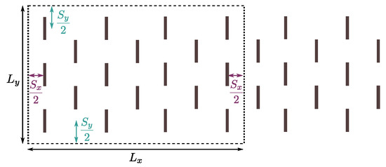
Figure 4.
Schematic of a representative control volume used to calculate the resultant force for an array of devices. Here, and are the length and the width of the control volume, respectively; meanwhile, the height, , is the same as the channel. In this example, the control volume encloses 18 devices, and comprises a volume that includes from the first to the seventh row of turbines.
We compared the resultant forces of a group of turbines obtained from the high-resolution numerical simulations with two analytical expressions, which are calculated by multiplying the force of a single device by the total number of turbines, , inside the control volume. In the first expression, we calculated the force by using the undisturbed velocity, , and the thrust coefficient, , the same as in Equation (3). On the other hand, in the second expression, we used the average velocity at the disk , which required a modified thrust coefficient, , to calculate the resultant force. In Figure 5, we show that the force calculated by using the undisturbed velocity overestimates the results, especially after the 3rd row. This is due to the fact that turbines starting at the 3rd row no longer experience the undisturbed velocity, . Instead, the resultant force calculated by using the averaged velocity of the disks, , provides a more accurate representation of the total force imposed by the set of turbines. We also observe that the analytical force goes up and down through the rows, which occurs because the density of turbines per unit area is smaller for rows with an even number of turbines. Furthermore, after the 6th row, all the total forces tended to remain constant, indicating that a fully developed solution can be assumed after six rows.
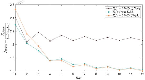
Figure 5.
Resultant force calculated by using control volumes that go from the first row of turbines through the last one (see Figure 4), per unit of mass (); ▪ analytic force calculated as the force of one actuator disk times the total number of devices in the farm; ⧫ analytic force calculated by using the average velocity at the location of the disks, , instead of the undisturbed velocity, ; • resultant force obtained from DES numerical simulations.
Due to the significant differences between the analytical solution using the undisturbed velocity, and the simulated resultant force showed in Figure 5, it is inferred that it is more accurate to use the local velocity to calculate the force of a set of turbines. However, we must consider that, in coarser-scale models, the only known velocity at the farm location is the grid-cell horizontally-averaged velocity (denoted here by ) at the hub height (subscript h): . Therefore, it is essential to modify the force calculation to represent a farm of turbines at larger-scale models. To achieve this, we proposed a thrust coefficient representative for an entire farm, , as follows:
where is calculated in the area occupied by the turbines. In this way, the new coefficient not only takes into account the wake interactions but also is based on information provided by coarse-scale models.
2.2.2. Thrust Coefficient for a Turbine Farm
To parameterize the thrust coefficient for an entire farm of turbines, , we studied the main parameters that dominate the interaction between the flow and the devices. Initially, we suggest that would depend on the distance among devices in the streamwise and spanwise directions, and , respectively; the disk diameter, D; and the size of the farm in the x and y directions, and . Experiments show that the ratio between the water depth, H, and the hub height, , is also an important variable to take into account since it can change considerably the velocity recovery downstream [18].
Another important factor is the angle between the flow and the turbines. Here, we only consider the optimal case, where the main flow direction is perpendicular to the rotor. In practice, one should take into account the fact that the thrust coefficient of turbines could be affected up to a for a yaw angles of [34]. The effect of bathymetry will not be included in the analysis of because it has been demonstrated that bedforms that can significantly alter the performance of the turbines are those that have length scales with an order of magnitude equal to or bigger than the radius of the disks [35,36], which is an unlikely scenario in large tidal channels.
For the purposes of this work, we used a staggered distribution for the turbines since this is the most commonly utilized configuration, and it is more efficient than when the disks are aligned [30,31]. We also considered the thrust coefficient for an individual device, , to normalize , in order to have a parameterization that works for any turbine. By performing numerical simulations, we studied the versatility of by using different values for the aforementioned parameters, and focused on the overall problem: . In non-dimensional form, we cast the problem as:
Previous works have highlighted the importance of not using the area density of the turbines, i.e., , since this assumption considers that a change in the streamwise distance would have the same effect as a change in the spanwise direction; this has been demonstrated as being inaccurate [37]. This is reason why the parameters and represent different dimensionless groups in Equation (8). The same is true for the size of the farm since the width and length of the farm independently affect the overall force, even though they have the same total area . The terms and in Equation (8) represent the farm size, and they can be interpreted as the number of rows and columns of devices.
2.2.3. Setup for Numerical Simulations
We simulated seven cases, and in each of them the turbines are distributed in a staggered pattern (same as in Figure 1 (i.e., odd rows have three turbines, and pairs, have two)). Since the focus of this research is to study finite-sized farms, the cases have only six rows. The cases vary the turbines’ separation in the streamwise () and spanwise () directions, as well as the ratio between the depth of the channel and hub height, . The simulations are summarized in Table 1.

Table 1.
Summary of the simulated cases.
Since our work is focused on tidal energy, we chose parameters according to the characteristics of the ocean and the TEC devices. For the diameter of the turbines, we used a typical value of m, with a hub height m. Regarding the thrust coefficient, we used the same value as for the validation case (i.e., ) to represent every device). In the ocean, Reynolds numbers can exceed , due to computational restrictions, we initially carry out this analysis with . We do not expect differences in to impact our results since it has been shown that increments of Reynolds numbers over do not have any significant effects on the wakes of actuator disks [38,39]; however, we highlight that we cannot ensure the same for real devices since they differ on the geometrical details of each specific design. As a new generation of TEC devices emerges, future work will focus on the effects of the Reynolds number for the entire tidal cycle. Concerning the turbulence intensity, we use an intermediate value equal to . For all the simulated cases, we used the same domain and the same grid resolution as summarized in Table 2.

Table 2.
Main variables common for all the simulated cases
3. Results and Discussion
Using the results from simulations C.1 through C.7, we calculate and study the sensitivity of due to changes in the lateral distance between devices the depth of the channel. From this analysis, we propose a relation between and the parameters listed in Equation (8). Finally, we provide a comparison with results from a previous investigation related to drag parameterizations of infinite farms.
3.1. Formulation of the Thrust Coefficient for Farms of Turbines
The solutions of the simulations in Table 1 are time-averaged, and we calculate the resultant force for different control volume configurations within the simulated domain (the same as in Section 2.2.1).
We observe that the effects on of changing the number of devices in the lateral direction are negligible (see Figure 6a). Actually, for all the shown cases, the coefficient only changes around when we go from two to four columns of turbines. This is reasonable because, regardless of how many columns of turbines are included, the undisturbed flow upstream will face the same total area of turbines (also known as the blockage area). For this reason, we eliminate from our parameterization. We have to mention that we do not show the case C.4 in Figure 6a because, in that situation, the devices are too laterally close, and it is not possible to isolate the effect of the columns of turbines to study them.
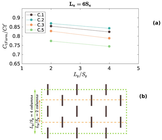
Figure 6.
variation of due to changes in the size of the farm in the spanwise direction, . The ratio can be interpreted as the number of columns of turbines; schematic of the control volumes used for calculating for two and four rows of turbines.
On the other hand, varies noticeably when the longitudinal length of the farm changes (see Figure 7a). When farms increase from two rows of turbines () to three rows (), decreases. Beyond this, remains almost constant as additional rows are included. For our parameterization, we do not consider the case of one row () since, in that situation, is undetermined, and one would expect the wake interactions to not play a strong role in the total effective thrust coefficient .
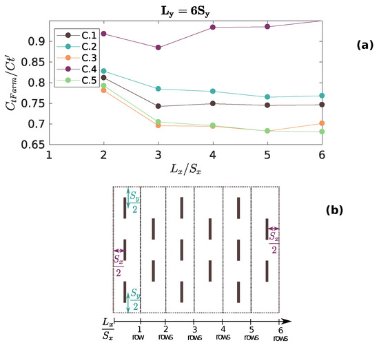
Figure 7.
variation of due to changes in the size of the farm in the streamwise direction, . The ratio can be interpreted as the number of rows of turbines; schematic of the control volumes used for calculating for various numbers of rows.
For studying the effects of , , and on , we divide the results into two cases: one for farms with exactly two rows, and another for farms with more than two rows. This distinction is used because of the difference observed previously in Figure 7, for the cases where , and .
In Figure 8a, the variation of as a function of streamwise separation between the devices is presented. We observe that, for farms with two rows, the thrust coefficient remains almost constant. We perform additional simulations with exactly two rows using even smaller values of , and remains independent of changes in . We also can see in Figure 8a that, for more than two rows, increases when increases. This is consistent with previous work for vegetation canopies [37], where the authors stated that the thrust coefficient should be maximum for isolated objects (i.e., ) because the obstacles or, in our case, the turbines, are completely unsheltered.
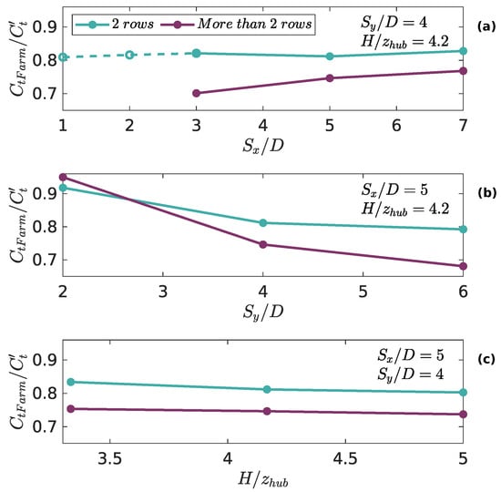
Figure 8.
Changes in due to the variation of: the streamwise distance between devices, ; the spanwise distance between devices, ; and the ratio between the depth of the channel and the hub height, . The results are divided into two cases: farms with two rows of turbines (light blue), and farms with more than two rows (purple). Since we do not observe a significant influence of on for farms with two rows, we perform extra simulations (marked with dashed lines), where we see remains insensitive to the distance in the streamwise direction.
In Figure 8b, it is observed that decreases when increases for farms with any number of rows. This is also consistent with Simón-Moral et al. [37], where it was noted that, when the devices are laterally closer, the average velocity inside the canopy is smaller, which results in a higher thrust coefficient. The aforementioned is reflected in Figure 7, where case C.4 is the one with the highest . The velocity inside the farm is especially low in staggered farms with laterally close devices since the flow is blocked by them. Another study [11] shows that the efficiency of a wide or deep farm monotonically increases when the lateral separation between turbines decreases towards the lowest limit (i.e., ); this is consistent with our results as well.
Regarding the ratio between the depth and the hub height (Figure 8c), we do not observe a significant change in , regardless of the number of rows. In fact, with an increment of in , we calculate a change of less than in . We conclude that does not play a role in our parameterization. However, we note that we can only ensure the validity of this result for cases where , and we acknowledge that this parameter could be important for representing devices that are installed closer to the free surface.
As a summary, we infer that is not a function of nor . We also observe that there are two regimes concerning the length of the farm: one for farms with exactly two rows of turbines, and the other for farms with more than two rows. In the former, is only a function of the lateral distance of the devices (). In the latter, is function of in addition to .
Considering the discussion above, we propose an analytical solution for which is characterized by two limiting cases:
- (I)
- For farms with two rows, the expression for is inversely proportional to the lateral distance between devices, . This value can go from , when the turbines are adjacent to each other, to for very laterally spaced farms, where one would expect the drag force to be additive since the wakes do not interact.
- (II)
- For farms with more than two rows, the dependence of is still inversely proportional to , but also decays exponentially with the distance between the devices in the stream-wise direction . An exponential decay is proposed because it tends to zero as (i.e., the devices get closer), which captures the fact that the flow cannot penetrate the farm. On the other hand, when the stream-wise distance between the devices increases, the exponential term tends towards unity, which is equivalent to saying that becomes independent of . This expression is similar to the one proposed by Simón-Moral et al. [37] for parameterizing canopies of vegetation.
Thus, we present the following expression for :
Here, , , , and are coefficients empirically calculated by minimizing the error in the difference between the data obtained from the simulations and that predicted by the proposed relation. The value of these coefficients could be improved by running more numerical simulations to have more sample points. The coefficient attenuates the growth of the exponential function, and yields a which reaches a value of 0.99 at roughly , meaning that, for streamwise separations larger than , the wake is essentially fully recovered. This is in agreement with various recovery distances reported in the literature [10,33,40].
With respect to the factors and in Equation (9), they can be interpreted as the limit of for very laterally spaced farms (i.e., when ). In this case, the average velocity at the center of the farm tends to be the same as the undisturbed velocity, so that we can assume:
In Figure 9 and Figure 10, we show the empirical solution proposed in Equation (9) with the results from the DES simulations. In both figures, we fix values of to observe how changes with variations in (Figure 9a and Figure 10a), and vice versa (Figure 9b and Figure 10b). As mentioned above, for farms with two rows, does not depend on , which is why in Figure 9a the lines are horizontal. Meanwhile, in Figure 9b, we see that all curves collapse despite different values of . For farms with more than two rows (Figure 10), we see that our expression for is capable of representing the effects of changing the distance between devices in both lateral directions.
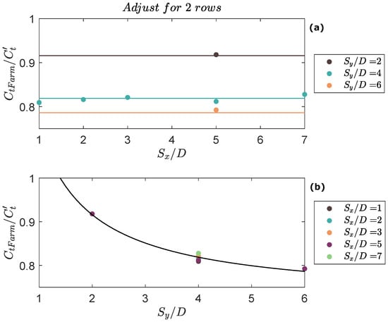
Figure 9.
, for farms with exactly two rows of turbines, versus the disk separation in: the streamwise direction, and in the spanwise direction. Continuous line: Empirical solution proposed in Equation (9). Dots: Results from DES numerical simulations.
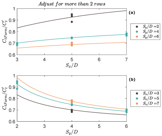
Figure 10.
, for farms with more than two rows of turbines, versus the disks separation in: the streamwise direction, and in the spanwise direction. Continuous line: Empirical solution proposed in Equation (9). Dots: Results from DES numerical simulations.
3.2. Comparison of Parameterization with Previous Work
To demonstrate the consistency of our parameterization with other studies, we compare our results with the parameterization proposed by Abkar and Porté-Agel [14]. As noted in the Introduction, the authors of Abkar and Porté-Agel [14] considered an infinite farm of turbines, and incorporated a correction factor, , to account for differences in the free-stream and horizontally-averaged velocities:
In their work, Abkar and Porté-Agel [14] showed that the implementation of can improve the representation of farms of turbines in larger scale models. Their approach was empirical, so was computed numerically for a wide variety of disk configurations. To compare our expression with the results of Abkar and Porté-Agel [14], we rewrite Equation (9) to incorporate into :
Since the parameterization of Abkar and Porté-Agel [14] was made for an infinite farm, we can assume that the flow reaches a fully developed state, which means that . The term in Equation (12) can be compared with the parameter by using the relation [25], where is an induction factor used by Abkar and Porté-Agel [14]. In this way, we can estimate from our analytical solution.
In Table 3, we show that, using the proposed expression, we retrieve values for with an error of less than in comparison with the results of Abkar and Porté-Agel [14]. The crucial difference with our work is that we are able to also take into account the effect of two different turbines configurations just by knowing the lateral distance between devices, without needing to run computationally expensive numerical simulations.

Table 3.
Comparison of the results of the parameter (Data from: Abkar and Porté-Agel [14]) with calculated by using our parameterization of .
4. Conclusions
In this work, we propose an expression for a new thrust coefficient, , which is meant to represent a finite-sized farm of TEC devices in ocean circulation models. Our primary objective is to include the variation of the resistance force due to the distribution of the devices. We use the hybrid DES turbulence model coupled with the actuator disk approach to simulate staggered farms of turbines by changing the lateral separation of the devices and the depth of the channel.
We validated the model by replicating the laboratory experiments shown in [30]. Despite the simple representation of the turbines, we can faithfully reproduce the velocity deficit downstream of the turbines. With these simulations, we calculate the resultant force of various farm sizes to detect which variables are more relevant in the representation of turbine arrangements at larger scales. We also analyze the way in which behaves under changes in device spacing, in order to propose an expression for this new coefficient.
Finally, we conclude that behaves differently for farms with exactly two rows, and farms with more rows. In the first scenario (farms with two rows), the lateral separation of the devices is the only variable required in the calculation of , mainly because it is primarily related to the area of the turbines which the flow faces when it enters to the farm. For laterally closer devices, increases monotonically until . For farms that have more than two rows, the streamwise distance between the devices becomes relevant too. This parameter is incorporated into the expression by using an exponential decay which goes from zero for farms with no space between rows (i.e., ) to unity for farms with highly spaced rows (i.e., ). We also conclude that is not a relevant variable in the representation of farms of turbines, at least when its value is equal or bigger than .
With the new proposed expression, it is possible to easily calculate a thrust coefficient for a finite farm of turbines, just by knowing the number of rows and the lateral separation of the devices. However, we highlight that before using our parameterization, a few notes are necessary:
- It is designed for staggered farms, where all the turbines occupy the same ground area.
- It does not consider a significant misalignment between the mean flow direction and the turbine axes.
- It is designed for devices that are installed at the bottom of the sea, and which do not interact with the free-surface.
Furthermore, we have to highlight that further simulations are necessary in order to improve the precision of the coefficients presented in the equation of .
Future work consists of implementing the coefficient into ocean circulation models such as FVCOM [41], where it is possible to simulate the tides and their interaction with the bathymetry in a larger temporal and spatial scale. By using these kinds of models, we could study the effects of farms of turbines in a more realistic domain with a flow that completes entire tidal cycles. Further development of the parameterization should be focused on using the capacity of ocean circulation models to solve the free-surface elevation to study the interaction with turbines installed closer to it, such as floating devices.
Author Contributions
Conceptualization, K.S.-R., C.E. and D.R.; methodology, K.S.-R., C.E. and D.R.; software, K.S.-R. and C.E.; validation, K.S.-R.; formal analysis, K.S.-R., C.E. and D.R.; investigation, K.S.-R., C.E. and D.R.; resources, C.E. and D.R.; data curation, K.S.-R.; writing—original draft preparation K.S.-R., C.E. and D.R.; writing—review and editing K.S.-R., C.E. and D.R.; visualization, K.S.-R.; supervision, C.E. and D.R.; project administration, K.S.-R., C.E. and D.R.; funding acquisition, K.S.-R., C.E. and D.R.
Funding
This research was funded by CONICYT-PCHA/Doctorado Nacional/2016-21160137 and the Marine Energy Research and Innovation Center (MERIC) project, CORFO 14CEI2-28228.
Acknowledgments
Powered@NLHPC: This research was partially supported by the supercomputing infrastructure of the NLHPC (ECM-02)
Conflicts of Interest
The authors declare no conflict of interest.
Abbreviations
The following abbreviations are used in this manuscript:
| DES | Detached-Eddy Simulations |
| LES | Large-Eddy Simulations |
| TEC | Tidal Energy Converter |
| RANS | Reynolds-Averaged Navier–Stokes |
| RMSE | Root Mean Square Error |
| RSR | Root mean square error-observations Standard deviation Ratio |
References
- IEA and World Bank. Sustainable Energy For All. Available online: https://datacatalog.worldbank.org/dataset/sustainable-energy-all (accessed on 18 March 2019).
- Hagerman, G.; Polagye, B.; Bedard, R.; Previsic, M. EPRI Guideline Methodology for Estimating Tidal Current Energy Resources and Power Production by Tidal In-Stream Energy Conversion (TISEC) Devices; Technical Report; Electric Power Research Institute: Palo alto, CA, USA, 2006. [Google Scholar]
- Tarbotton, M.; Larson, M. Canada Ocean Energy Atlas Phase 1: Potential Tidal Current Energy Resources Analysis Background; Canadian Hydraulics Centre: Ottawa, ON, Canada, 2006. [Google Scholar]
- Robins, P.E.; Neill, S.P.; Lewis, M.J.; Ward, S.L. Characterising the spatial and temporal variability of the tidal-stream energy resource over the northwest European shelf seas. Appl. Energy 2015, 147, 510–522. [Google Scholar] [CrossRef]
- Li, D.; Yao, Y.; Chen, Q.; Ye, Z. Numerical simulation of tidal current energy in Yangtze Estuary-Hangzhou Bay, China. In Proceedings of the OCEANS 2015, Genova, Italy, 18–21 May 2015; pp. 1–6. [Google Scholar] [CrossRef]
- Yang, Z.; Wang, T.; Copping, A.; Geerlofs, S. Modeling of in-stream tidal energy development and its potential effects in Tacoma Narrows, Washington, USA. Ocean Coast. Manag. 2014, 99, 52–62. [Google Scholar] [CrossRef]
- Nash, S.; O’Brien, N.; Olbert, A.; Hartnett, M. Modelling the far field hydro-environmental impacts of tidal farms—A focus on tidal regime, inter-tidal zones and flushing. Comput. Geosci. 2014, 71, 20–27. [Google Scholar] [CrossRef]
- Wang, T.; Yang, Z. A modeling study of tidal energy extraction and the associated impact on tidal circulation in a multi-inlet bay system of Puget Sound. Renew. Energy 2017, 114, 204–214. [Google Scholar] [CrossRef]
- Piano, M.; Robins, P.E.; Davies, A.G.; Neill, S.P. The Influence of Intra-Array Wake Dynamics on Depth-Averaged Kinetic Tidal Turbine Energy Extraction Simulations. Energies 2018, 11, 2852. [Google Scholar] [CrossRef]
- Myers, L.; Bahaj, A. An experimental investigation simulating flow effects in first generation marine current energy converter arrays. Renew. Energy 2012, 37, 28–36. [Google Scholar] [CrossRef]
- Nishino, T.; Willden, R.H.J. The efficiency of an array of tidal turbines partially blocking a wide channel. J. Fluid Mech. 2012, 708, 596–606. [Google Scholar] [CrossRef]
- Stansby, P.; Stallard, T. Fast optimisation of tidal stream turbine positions for power generation in small arrays with low blockage based on superposition of self-similar far-wake velocity deficit profiles. Renew. Energy 2016, 92, 366–375. [Google Scholar] [CrossRef]
- Fitch, A.C.; Olson, J.B.; Lundquist, J.K.; Dudhia, J.; Gupta, A.K.; Michalakes, J.; Barstad, I. Local and Mesoscale Impacts of Wind Farms as Parameterized in a Mesoscale NWP Model. Mon. Weather Rev. 2012, 140, 3017–3038. [Google Scholar] [CrossRef]
- Abkar, M.; Porté-Agel, F. A new wind-farm parameterization for large-scale atmospheric models. J. Renew. Sustain. Energy 2015, 7, 013121. [Google Scholar] [CrossRef]
- Calaf, M.; Meneveau, C.; Meyers, J. Large eddy simulation study of fully developed wind-turbine array boundary layers. Phys. Fluids 2010, 22, 015110. [Google Scholar] [CrossRef]
- Calaf, M.; Parlange, M.B.; Meneveau, C. Large eddy simulation study of scalar transport in fully developed wind-turbine array boundary layers. Phys. Fluids 2011, 23, 126603. [Google Scholar] [CrossRef]
- Porté-Agel, F.; Lu, H.; Wu, Y.T. Interaction between Large Wind Farms and the Atmospheric Boundary Layer. Procedia IUTAM 2014, 10, 307–318. [Google Scholar] [CrossRef]
- Aghsaee, P.; Markfort, C.D. Effects of flow depth variations on the wake recovery behind a horizontal-axis hydrokinetic in-stream turbine. Renew. Energy 2018, 125, 620–629. [Google Scholar] [CrossRef]
- Kolekar, N.; Banerjee, A. Performance characterization and placement of a marine hydrokinetic turbine in a tidal channel under boundary proximity and blockage effects. Appl. Energy 2015, 148, 121–133. [Google Scholar] [CrossRef]
- Spalart, P.; Allmaras, S. A one-equation turbulence model for aerodynamic flows. Rech. Aerosp. 1994, 1, 5–21. [Google Scholar]
- Escauriaza, C.; Sotiropoulos, F. Reynolds Number Effects on the Coherent Dynamics of the Turbulent Horseshoe Vortex System. Flow Turbul. Combust. 2011, 86, 231–262. [Google Scholar] [CrossRef]
- Escauriaza, C.; Sotiropoulos, F. Initial stages of erosion and bed form development in a turbulent flow around a cylindrical pier. J. Geophys. Res.-Earth 2011, 116. [Google Scholar] [CrossRef]
- Escauriaza, C.; Sotiropoulos, F. Lagrangian model of bed-load transport in turbulent junction flows. J. Fluid Mech. 2011, 666, 36–76. [Google Scholar] [CrossRef]
- Gajardo, D.; Escauriaza, C.; Ingram, D.M. Capturing the development and interactions of wakes in tidal turbine arrays using a coupled BEM-DES model. Ocean Eng. 2019, 181, 71–88. [Google Scholar] [CrossRef]
- Burton, T.; Sharpe, D.; Jenkins, N.; Bossanyi, E. Wind Energy Handbook; John Wiley & Sons, Ltd.: Chichester West Sussex, UK, 2011; ISBN 0-471-48997-2. [Google Scholar]
- Blackmore, T.; Batten, W.M.J.; Bahaj, A.S. Influence of turbulence on the wake of a marine current turbine simulator. Proc. R. Soc. A-Math. Phys. 2014, 470, 20140331. [Google Scholar] [CrossRef] [PubMed]
- Lloyd, T.P.; Turnock, S.R.; Humphrey, V.F. Assessing the influence of inflow turbulence on noise and performance of a tidal turbine using large eddy simulations. Renew. Energy 2014, 71, 742–754. [Google Scholar] [CrossRef]
- Smirnov, A.; Shi, S.; Celic, I. Random flow generation technique for Large eddy simulations and particle-dynamics modeling. J. Fluids Eng. 2001, 123, 359–371. [Google Scholar] [CrossRef]
- Chamorro, L.P.; Porté-Agel, F. Turbulent Flow Inside and Above a Wind Farm: A Wind-Tunnel Study. Energies 2011, 4, 1916–1936. [Google Scholar] [CrossRef]
- Markfort, C.D.; Zhang, W.; Porté-Agel, F. Turbulent flow and scalar transport through and over aligned and staggered wind farms. J. Turbul. 2012, 13. [Google Scholar] [CrossRef]
- Wu, Y.T.; Porté-Agel, F. Simulation of Turbulent Flow Inside and Above Wind Farms: Model Validation and Layout Effects. Bound.-Layer Meteorol. 2013, 146, 181–205. [Google Scholar] [CrossRef]
- Moriasi, D.N.; Arnold, J.G.; Van Liew, M.W.; Bingner, R.L.; Harmel, R.D.; Veith, T.L. Model evaluation guidelines for systematic quantification of accuracy in watershed simulations. Trans. ASABE 2007, 50, 885–900. [Google Scholar] [CrossRef]
- Stallard, T.; Collings, R.; Feng, T.; Whelan, J. Interactions between tidal turbine wakes: Experimental study of a group of three-bladed rotors. Philos. Trans. R. Soc. A 2013, 371, 20120159. [Google Scholar] [CrossRef]
- Frost, C.H.; Evans, P.S.; Harrold, M.J.; Mason-Jones, A.; O’Doherty, T.; O’Doherty, D.M. The impact of axial flow misalignment on a tidal turbine. Renew. Energy 2017, 113, 1333–1344. [Google Scholar] [CrossRef]
- Hill, C.; Musa, M.; Guala, M. Interaction between instream axial flow hydrokinetic turbines and uni-directional flow bedforms. Renew. Energy 2016, 86, 409–421. [Google Scholar] [CrossRef]
- Musa, M.; Hill, C.; Sotiropoulos, F.; Guala, M. Performance and resilience of hydrokinetic turbine arrays under large migrating fluvial bedforms. Nat. Energy 2018, 3, 839–846. [Google Scholar] [CrossRef]
- Simón-Moral, A.; Santiago, J.L.; Krayenhoff, E.S.; Martilli, A. Streamwise Versus Spanwise Spacing of Obstacle Arrays: Parametrization of the Effects on Drag and Turbulence. Bound.-Layer Meteorol. 2014, 151, 579–596. [Google Scholar] [CrossRef]
- Sørensen, J.N.; Shen, W.Z.; Munduate, X. Analysis of wake states by a full-field actuator disc model. Wind Energy 1998, 1, 73–88. [Google Scholar] [CrossRef]
- Mikkelsen, R.F. Actuator Disc Methods Applied to Wind Turbines. Ph.D. Thesis, Technical University of Denmark, Kongens Lyngby, Denmark, 2004. [Google Scholar]
- Chen, Y.; Lin, B.; Lin, J.; Wang, S. Experimental study of wake structure behind a horizontal axis tidal stream turbine. Appl. Energy 2017, 196, 82–96. [Google Scholar] [CrossRef]
- Chen, C.; Liu, H.; Beardsley, R.C. An Unstructured Grid, Finite-Volume, Three-Dimensional, Primitive Equations Ocean Model: Application to Coastal Ocean and Estuaries. J. Atmos. Ocean. Technol. 2003, 20, 159–186. [Google Scholar] [CrossRef]
© 2019 by the authors. Licensee MDPI, Basel, Switzerland. This article is an open access article distributed under the terms and conditions of the Creative Commons Attribution (CC BY) license (http://creativecommons.org/licenses/by/4.0/).