1. Introduction
Modern power systems are facing unprecedented levels of renewable energy penetration motivated by government targets and potential reductions in cost per MWh. The introduction of large scale wind power generation may lead to the decommissioning of conventional synchronous generators which will have a negative impact on the stability of the system of a whole. Without the large rotating masses and the associated inertia that these synchronous generators provide, the frequency of the system will become more sensitive to disturbances. Additionally, type-3 and type-4 variable speed wind turbines which are the most common topologies in new developments [
1] are either partially or fully decoupled from the grid through power electronic converters, meaning that their inertia contributions cannot be ‘seen’ by the wider network. As the penetration of low inertia wind energy increases, the effect on power system stability becomes an important issue which needs to be analysed [
2].
The concept of synthetic inertia is nothing new. Unlike a synchronous generator, the kinetic energy stored in the wind turbine blades cannot be readily accessed and can only be released through control action. The term synthetic comes from the fact that there is no instantaneous response to a drop in frequency in the wider network and all action is achieved through the power electronic converter. The share of wind power is now so large that system operators are revising their grid codes such that wind farms require frequency control capabilities in specific conditions [
3].
This paper looks to gain insight into how different synthetic inertia control strategies compare to each other in the context of small-signal stability by analysing the oscillatory electromechanical modes between synchronous generators. Low frequency oscillation of local modes between nearby generators and inter-area modes between generators in different areas can have detrimental effects on transmission capacity and stability of the system as a whole [
4]. It is hypothesised that, although synthetic inertia control strategies provide the system with some much needed frequency support, the different methods of achieving this may have unintended downsides in reducing the damping ratio of the system and driving the network into the realms of instability.
1.1. Synthetic Inertia
This paper will focus on two methods of synthetic inertia provision, both of which work by providing an artificially manipulated set-point to the active power controller. The effect of this new set-point is to release a portion of the kinetic energy stored in the rotor and provide active power at the expense of a reduction in rotational speed. Clearly, this method cannot be sustained indefinitely due to the finite quantity of kinetic energy available, but to satisfy existing and proposed grid codes, only a small percentage of rated power needs to be provided for a limited time, typically below ten percent of the rated capacity [
5,
6,
7]. For the purposes of this work, this value is exaggerated for demonstration purposes up to a maximum of 20% of the rated wind farm capacity. Whilst not impossible, this approach is unrealistic in a real-world environment but will be useful in demonstrating the core concepts.
The first method of synthetic inertia control, shown in
Figure 1a, is a one-loop design based on the deviation of the system frequency from the nominal value [
8,
9]. This scheme is termed droop control and regulates the active power output from a wind turbine proportional to the change in frequency. There is a linear relationship between active power and frequency, and this control scheme adjusts the power set-point according to the linear characteristic in (
1).
where
is the new frequency,
is the initial operating point and R is the droop constant.
The second control strategy to be considered is the two-loop design shown in
Figure 1b. This scheme provides a modified power reference which is proportional to frequency deviation and lasts until nominal frequency is restored.The first loop acts when the rate of change of frequency is high, while the
loop has a strong effect when the system frequency differs greatly from the nominal value. The values of K1 and K2 are selected based on the desired level of synthetic inertia provided by the DFIG. The effects of changing K1 and K2 are discussed in more detail in [
10].
1.2. Modelling
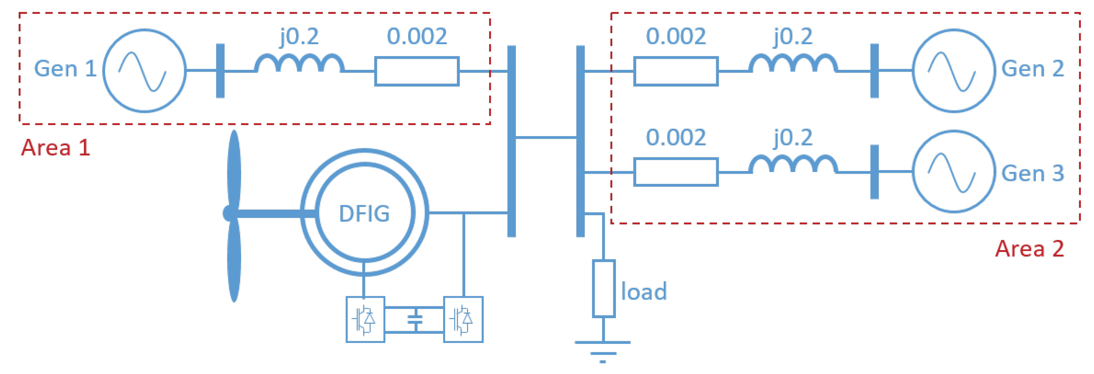
The model used for simulation is based on a two-area network featuring three synchronous machines and a wind farm. In the absence of an infinite bus, a load must be connected to the central bus to balance the power flow and maintain synchronism. These components are connected to each other via a set of network equations which define the admittance matrix of the system. A schematic layout of the system is shown in
Figure 2 which identifies the two areas.
Table A1 and
Table A2 in
Appendix A give the parameters of the machines.
The machines are sized such that generator 1 is five times larger in capacity than generators two and three, rated at 1000, 200 and 200 MW, respectively. Generator 1 is fitted with a simple governor to regulate rotor speed via an applied torque and to fix the network frequency at the nominal value. Generator 1 is therefore termed the balancing machine. The DFIG represents an entire wind farm of identical individual turbines with an aggregated power of 100 MW.
The network model uses the transient model of a synchronous generator in the dq-reference frame in which the stator dynamics are neglected. The resulting set of differential equations are fourth order: two differential equations describe the rotor dynamics and the remaining two are used to describe the rotor speed and angle [
11]. The DFIG is modelled as a fifth order system in the dq-reference frame. Since every element of the network is modelled in dq, the effects of the PLL can be neglected. This is because operating in the dq reference frame is equivalent to having an ideal PLL. The full set of network equations and parameters are provided in
Appendix A.
Control of the DFIG is achieved by directly manipulating the rotor voltages in the dq-frame, negating the need to model the back-to-back converter. This method is based on the internal mode control presented in [
12]. Since this paper is only focused on the active power controller which operates entirely in the d-axis, further simplifications can be made by omitting any q-axis components relating to reactive power.
2. Linearisation
Small-signal stability defined in the context of a power system is the ability to maintain synchronism when subjected to small perturbations [
13]. The term ‘small’ implies that the equations describing the response may be linearised for analysis, which is the focus of this section.
The power system under consideration is given by a set of n linearly independent state variables of the form in (
2), where
are the state variables,
are the inputs to the model and t is time. The complete set of differential equations is provided in
Appendix A. The state variables are a combination of physical quantities such as angle and speed, and other more abstract mathematical variables associated with the differential equations that describe the dynamics of the system [
13].
To begin the linearisation process, a set of equilibrium points must first be defined. These are the points where all of the derivative terms are simultaneously zero, implying that the system is at rest and all of the variables are constant with respect to time. Mathematically, this implies that
, with
being an operating point. Due to the complexity of a multi-machine system, the equilibrium points of the model considered in this paper are determined from simulation. After a sufficiently long settling time, a snapshot is taken of the state variables when they are in steady-state and saved to file. This is done multiple times for different operating conditions and control strategies until a complete set of equilibrium points exist for all scenarios. The system state equations are then obtained by linearisation at an equilibrium point:
where
Here,
is rotor speed of the doubly-fed induction generator,
comes from the integral term in the power controller,
are the fluxes,
are from the transfer functions of the governor,
and
are the angle and speed of the synchronous generators respectively and
are the two-axis transient emfs of the synchronous generators. For
n = 3 generators, these states form a 21-order system.
Small-signal stability analysis is concerned with the eigenproperties of the Jacobian matrix
, which is of the form in (
7). The entries in
give the coupling relationships between each of the dynamic processes [
14]. The eigenvalues of
are of the form in (
8).
For a complex pair of eigenvalues, the real component gives the damping and the imaginary component gives the frequency of oscillation. The frequency of oscillation is given by (
9) and the damping ratio is given by (
10). The damping ratio is of particular importance as this determines the rate of decay of the oscillations. A high damping ratio implies that any oscillations away from the static equilibrium will decay quickly, whereas a low damping ratio implies the opposite. A high value of
is desirable in the context of small-signal stability. It can be seen from Equation (
10) that the value of
is largely dependant on the real component of a particular eigenvalue, such that a more-negative real component implies a higher damping ratio. This is analogous to the position of poles in control theory, where the system is stable if the poles are in the left hand plane, and a more negative real component results in a faster response. Note that it is also a necessary condition for stability that all eigenvalues have a negative real part.
There is no one-to-one relationship between any single eigenvalue and a particular state because they each belong to the system as a whole. It is therefore necessary to define the participation matrix
which provides a numerical score of a particular eigenvalue against a specific state. The participation matrix is generated from the matrices of right and left eigenvalues,
and
respectively. Note that it is standard practice to normalise these matrices such that
.
where the right and left eigenvectors are given by Equations (
13) and (
14) respectively.
The modal matrices
and
are then used to form the participation matrix
, the entries of which will be used to determine the dominant eigenvalues for each state.
kth row, ith column of modal matrix .
ith row, kth column of modal matrix .
3. Results
The simulation will be run under three conditions in three different scenarios: no inertia control; one-loop control from
Figure 1a and two-loop control from
Figure 1b, for the three network scenarios defined below. The eigenproperties of the resulting state matrix will then be analysed to infer the behaviour of each control strategy in the wider context of the network.
Base case—system is operating normally;
Heavy load—the governor fitted to generator 1 is limited such that it can no longer provide additional power. The grid is now at full capacity and any imbalance between generation and load will be strongly reflected in the frequency characteristic;
Weak interconnection—the tie-line connecting generator 1 to the rest of the system is reduced in strength to represent a longer transmission line and a weaker grid.
3.1. Scenario 1—Base Case
For the base case of the model without any synthetic inertia control, the eigenvalues of
are given in
Table 1, which shows the real and imaginary components, the frequency and damping ratio of each oscillatory mode and the associated dominant states as determined from the participation matrix.
From
Table 1 it can be seen that there are several eigenvalues with rotor speed and angle as the dominant states. The terms
are used to specify the generators involved in each mode such that
affects all three generators from both areas, whereas
only applies to generators 2 and 3 which are confined to the same area. This demonstrates the concept of inter-area and local-area modes.
Since the mechanical dynamics of a DFIG are decoupled from the electric grid, they therefore do not participate in the modes of oscillation and instead interact either by displacing synchronous generators, or by interaction of the controllers with the damping torque of large generators [
15]. This absence of coupling between the DFIG wind turbine and the synchronous generators is shown in
Table 1. In the absence of synthetic inertia control the terms in matrix
which couple the DFIG to the synchronous generators are zero, meaning that the state variables of a wind turbine do not contribute to the electromechanical oscillations between synchronous generators. When the DFIG is made to behave more like a synchronous machine through synthetic inertia provision, a coupling is introduced such that the DFIG contributes to these oscillations [
16,
17]. However, this effect is strongly tied to the dynamics of the PLL and since this paper uses a purely dq-reference frame, the coupling is not seen even when synthetic inertia control is introduced [
14].
In scenario 1, the system appears as in
Figure 2. The simulation is initialised for each of the three control strategies using their respective equilibrium points for linearisation which results in a state-space model. The time-domain response of the three control designs can be seen in
Figure 3, which shows an impulse being sent to the mechanical torque of generator 3 and the corresponding effect this has on the rotor speed and hence electrical frequency. One-loop control shows improved recovery to a frequency disturbance as compared to no-control, while the two-loop improves on this with an even more reduced frequency nadir.
It can be seen from
Table 1 that the system is stable, characterised by the negative real parts of each eigenvalue. There are two rotor angle modes of oscillation: the inter-area mode of G(1,2,3) and the local-area mode between G(2,3) identified from the table as
and
. The mode shapes are plotted in
Figure 4a which shows the swinging of generator 1 with generators 2 and 3, and
Figure 4b which shows the swinging of generator 2 with generator 3.
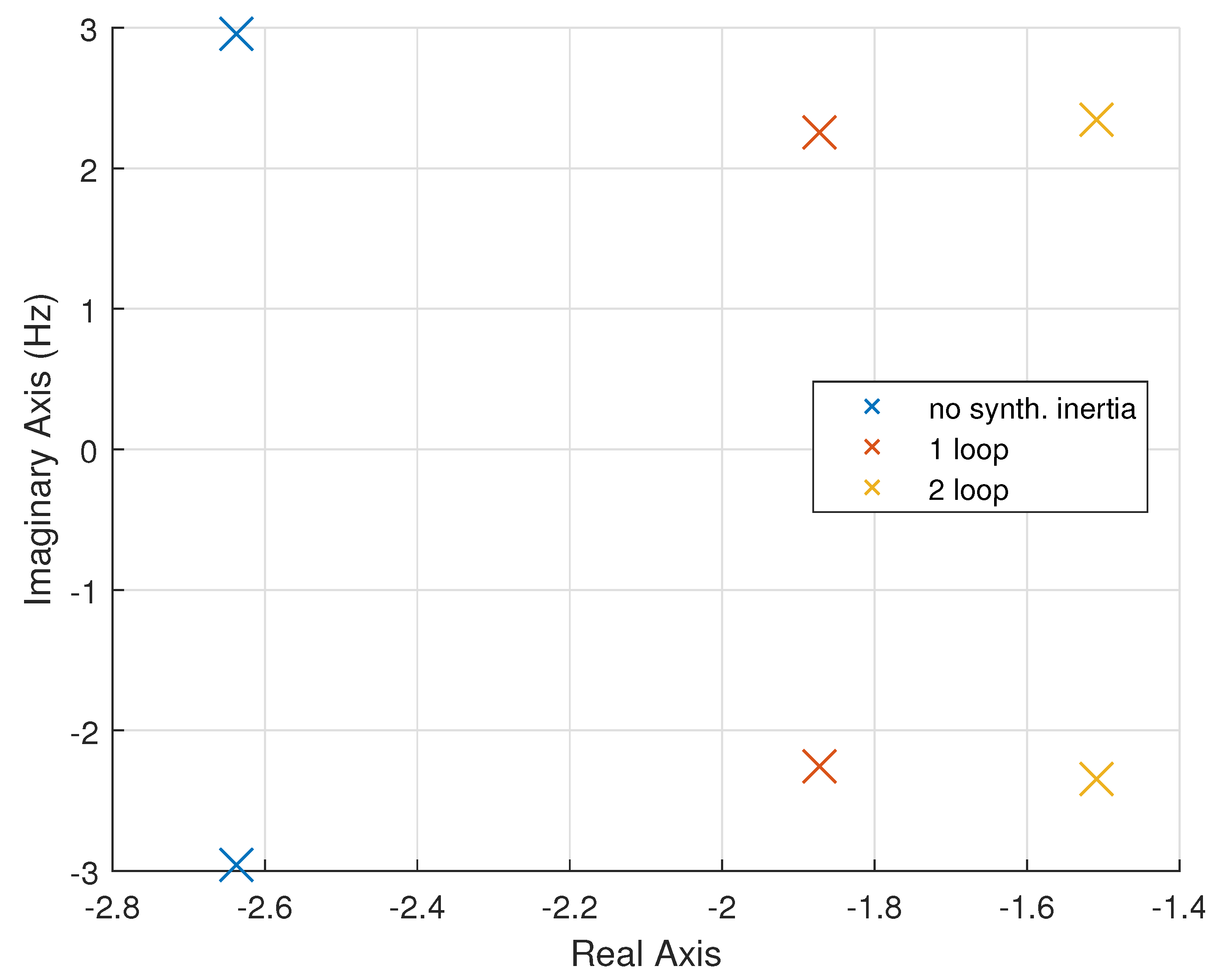
Figure 5 is a pole plot displaying the trajectories of the eigenvalues between the three control strategies. The cluster of eigenvalues to the left of the graph, with real part
, are those related to the local area mode. These are unchanged between the three synthetic inertia control strategies showing that the DFIG has no effect on local mode participation. The remaining eigenvalues belong to the inter-area mode. As the control strategies are introduced, the eigenvalues shift further to the right hand side representing a decreased stability characterised by a reduction in damping ratio. These are given in
Table 2 which shows how damping is reduced with the introduction of synthetic inertia. The damping ratio is reduced from 0.152 in the no control run, to 0.151 and then 0.130 in the one-loop and two-loop runs respectively. Similarly, the real component of the eigenvalue decreases from −2.335, to −2.298 then −2.023. The results suggest that the more effective the synthetic inertia control becomes, the lower the damping ratio for inter-area oscillations.
3.2. Scenario 2—Heavy Load
As described in the previous section, scenario 2 investigates the effect of different synthetic inertia schemes on a heavily loaded network. In this simulation, the balancing mechanism is removed from generator 1 such that the governor can no longer command the release of extra power in the event of a disturbance. When one of the other generators is taken offline, as in this simulation, the frequency does not recover and instead reduces to a new equilibrium.
The effects of synthetic inertia control on the electromechanical oscillations of the system are very similar to those in the base case of scenario 1. Once again, the local-area modes are unaffected and have therefore been omitted from any further analysis. The same pattern of reduced damping of the inter-area mode can be seen in
Table 3. As the control strategies become more sophisticated, the system becomes less stable. The pole-plot in
Figure 6 visualises the trend in
Table 3 and shows a clear shift to the right.
3.3. Scenario 3—Weak Grid
The final scenario investigates the effect of a weak grid on the system eigenvalues. Governor action is restored to generator 1 but the tie-line connecting generator 1 to the rest of the network is reduced in strength. This is achieved by increasing the value of the impedance to simulate a longer transmission line. Such lines are common when a distant generating station must be connected to a load centre over a considerable distance. The impedance between the bus at generator 1 and the central has been increased from the initial value of to , representing a three-fold increase in impedance.
The effect on the system eigenvalues can be seen in
Figure 7. Unsurprisingly, the system begins much less damped than the base case of scenario 1. The eigenvalues find themselves further to the right hand side towards increasing instability due to the weak grid criterion which has reduced the overall damping of all oscillations. As the control strategies are applied, the same pattern of reduced damping ratios can be seen to recur.
Table 4 shows that the damping ratio of the inter-area mode is reduced from 0.133 to 0.131 then to 0.102 for the no-control, 1-loop and 2-loop systems respectively.
4. Conclusions
This work has explored the effects of two different methods of synthetic inertia provision on small-signal stability in the context of a power system. A three-generator model with an added wind-farm was developed for the sole purpose of linearisation and small-signal analysis was conducted to explore the eigenproperties of different controller topologies and their effects on the electromechanical oscillations between generators. Three network scenarios were identified and tested, these being: base case; heavily loaded system, and a weaker grid.
The results show a trend of decreasing small-signal stability as synthetic inertia is introduced, with the more sophisticated two-loop synthetic inertia controller showing the greatest reduction. These results are shown in
Figure 5,
Figure 6 and
Figure 7 and
Table 2,
Table 3 and
Table 4, where the trajectories of the eigenvalues demonstrate a decreasing damping ratio and a less-negative real part. The base case, heavy load and weak grid simulations all mirror this effect. This suggests that the more a DFIG tries to emulate the action of a synchronous generator, the more it participates in inter-area oscillations. Overall, this has been characterised by a reduction in system damping ratio relating to those eigenvalues dominant to the shared mechanical modes of the synchronous generators.
This study has focused on modelling and simulation, yet the real-world applications of this study may present themselves in future electrical networks between the participation of wind farms in synthetic inertia provision. There may exist a trade-off between the degree of participation in frequency response and the greater instability associated with electromechanical oscillations. As the penetration of low-inertial renewable energy systems increases, it is likely that the phenomena of coupled oscillatory modes will become more apparent.


