Minimum Short Circuit Ratio Requirement for MMC-HVDC Systems Based on Small-Signal Stability Analysis

Abstract

This paper determines the minimum short circuit ratio (SCR) requirement for a modular multilevel converter based high-voltage direct current (MMC-HVDC) transmission systems. Firstly, a simplified model of MMC is introduced; the MMC is represented by its AC and DC side equivalent circuit. Next, by linearizing the MMC subsystem and the DC network subsystem, the deduction of the small-signal models of MMC subsystem, the small-signal model of the DC network and MMC-HVDC are carried out successively. Thirdly, the procedure for determining the minimum SCR requirement of MMC-HVDC is described. Finally, case studies are performed on a two-terminal MMC-HVDC system under four typical control schemes. The results show that the restraint factors for the rectifier MMC is predominantly the voltage safety limit constraint, and the restraint factors for the inverter MMC are mainly the phase locked loop (PLL) or the outer reactive power controller. It is suggested that the minimum SCR requirement for the sending and the receiving systems should be 2.0 and 1.5 in the planning stage.

1. Introduction

Recently, the modular multilevel converter based high-voltage direct current (MMC-HVDC) system has drawn significant attention from both the industry and academia. As a new breed of voltage-sourced converter (VSC), MMC outperformed the Line Commutated Converter (LCC) thanks to the decoupled control of active and reactive powers, the low harmonic voltages, the flexible scalability and the elimination of commutation failure [1,2,3,4]. MMC-HVDC has been widely used in transmission and distribution applications, such as wind farm connection, multi-terminal operation, and passive network power supply [5,6,7].

In the planning stage, one of the most important characteristics for the connected AC system is the short circuit ratio (SCR). For the LCC-HVDC, detailed research has been carried out by CIGRE and IEEE in which the AC system strength is categorized by the SCR [8,9]. The AC systems with SCR less than two are defined as very low SCR systems because the connected LCC cannot operate in a consistently stable manner [8]. For MMC-HVDC, there is no commonly accepted quantitation standard for describing the strength of the connected AC system, and there are no commonly accepted answers to the following two questions: (1) What are the minimum SCR requirements for the rectifier and the inverter MMC-HVDC station to transmit rated active power, respectively? and (2) Does the minimum SCR requirement vary with different control schemes?

As pointed out in [10], the steady-state power flow constraint, the small-signal stability constraint and the transient stability constraint should be all satisfied if MMC-HVDC (VSC-HVDC) could operate stably. To determine the minimum SCR under the third constraint, a time-domain simulation of certain faults is the conventional method, given the lack of a mature analytical method. Therefore, research on the minimum SCR is usually based on the former two constraints.

By using a Thevenin voltage source, the maximum available power (MAP) of VSC is plotted, and determines how the MAP is influenced by the SCR of the connected AC system, the angle of AC system impedance, the limitation on the internal voltage of the converter, and the reactive power support [11,12]. In [13], the minimum SCR for MMC-HVDC is calculated based on the steady-state power flow constraint. Because the dynamics of the converter is neglected, the results using the steady-state power flow constraint tend to be optimistic, and the results of [11,12,13] are only the ideal theoretical minimum SCR requirements. Recently, the small-signal stability analysis has drawn great attention in academia, with which a stricter minimum SCR requirement could be calculated. An eighth-order small-signal model of a VSC connected to weak AC system is derived in [14]; the results illustrate that the dynamics of PLL and the AC filter are crucial components for system stability. On the basis of the small-signal model, the influence of SCR and the phase-locked loop (PLL) on VSC was studied, and the connected AC systems with a SCR lower than 1.3 are defined as weak systems [15]. By studying the stability difference between MMC and VSC, the maximum power transmission capability of MMC could approach VSC by adjusting the PI parameters of PLL [16]. The small-signal stability of MMC is analyzed under the rectifier and the inverter mode, and the calculated minimum SCR of rectifier/inverter is 1.28–1.72/2.84–3.04 [17]. The explicit mathematical expression for the VSC system eigenvalues is derived based on reduced order model in [18], and result shows that the small signal stability of the system is significantly affected by the AC system strength (SCR) and PLL parameters. It is pointed out in [19] that the connected AC system could be considered weak if its SCR is less than 2.0 for VSCs with the classic vector current control scheme, while the virtual synchronous generator control scheme is especially suitable for weak system connections.

Generally speaking, existed small-signal stability analysis based method has the space for improvement considering the following three aspects: First, detailed high-order, small-signal model of MMCs with internal dynamics were usually adopted [20], which are not suitable for system-level planning studies. The high-order, small-signal model necessitates substantial requirements for modeling and computation resources, and its applicability in the system planning stage is limited. Second, one-terminal MMC with ideal DC source was usually adopted for calculating the minimum SCR, regardless of the dc network and other converter stations. Third, existed work mainly focused on the influence on small signal stability by controller parameters under single control scheme, influence on small signal stability by different control schemes has not been considered.

To overcome the aforementioned shortness of the existed research, improvements of this paper are made according to the following three aspects: (1) Derive the small-signal model of MMC-HVDC based on the simplified model of MMC; the internal dynamics of the MMC such as the circulating current is ignored to achieve computational efficiency; (2) Analysis is carried out using a two-terminal MMC-HVDC; the DC side of an MMC is connected to another MMC through the DC line as opposed to an ideal DC voltage source; in comparison with the MMC with an ideal DC voltage source, the model in this paper is more realistic and provides more reasonable results; (3) Four different control schemes are analyzed and compared, which provides more comprehensive results than a single control scheme.

The outline of this paper is as follows: Section 2 discusses the theory and introduces the simplified model of MMC for determine the minimum SCR requirement. Section 3 discusses the deduction of a small-signal model for MMC-HVDC. Section 4 describes the procedure of the proposed methodology. The case studies have been conducted on a 2-terminal MMC-HVDC system with four typical control schemes in Section 5. Section 6 is the concluding section.

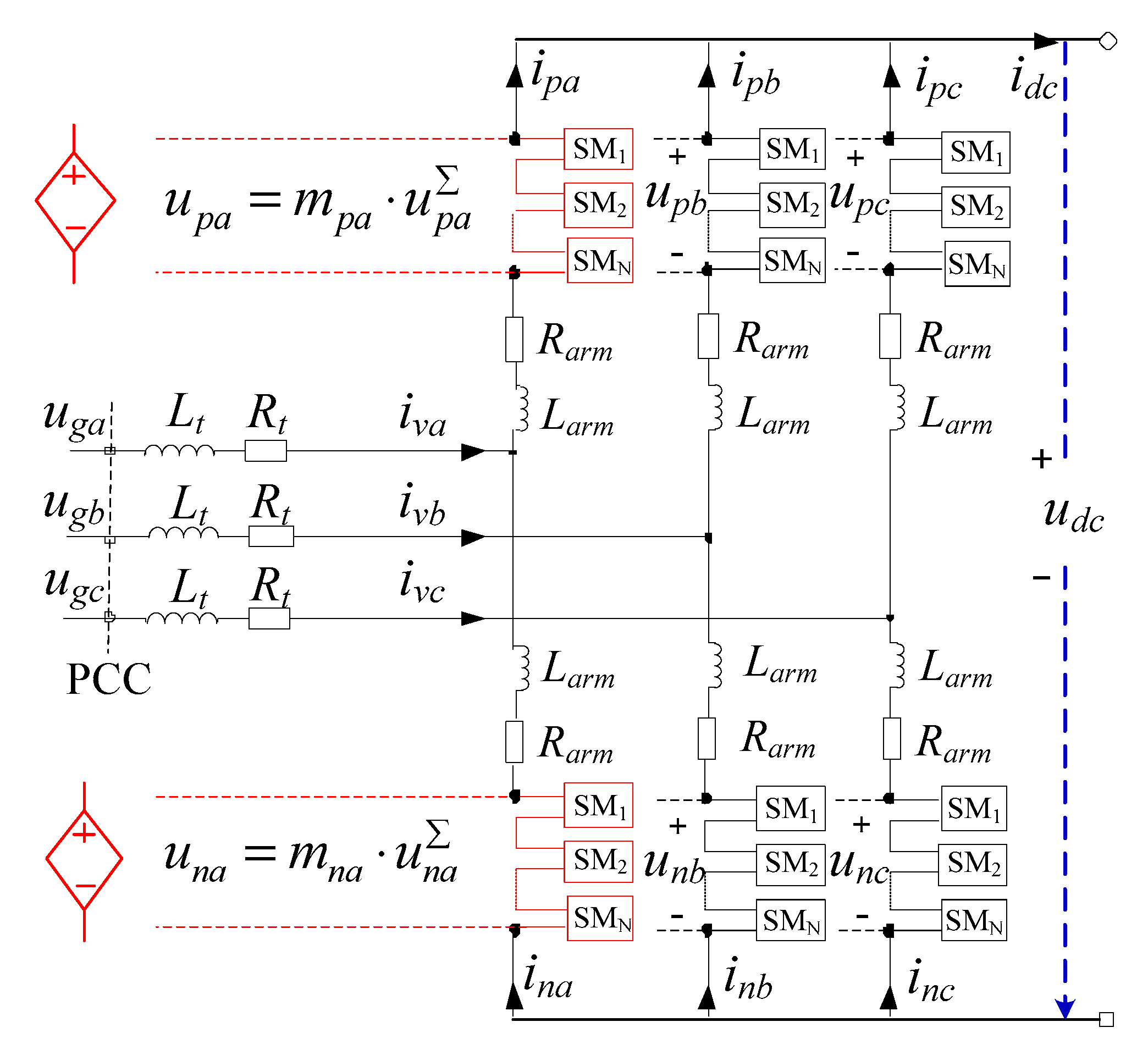
2. Theory and Simplified Model of Modular Multilevel Converter (MMC)

The structure of the MMC is illustrated in Figure 1. The converter consists of six arms; the upper and lower arms in the same phase form a phase unit. Each arm consists of two parts, i.e., N series-connected identical sub-modules (SMs) and an arm inductor L_arm. The equivalent arm resistor, the equivalent transformer inductor and resistor are denoted as R_arm, L_t and R_t, respectively. For simplicity, only half bridge SMs [3] are considered in this paper.

As seen in Figure 1, u_rj and i_rj are the arm voltage and the arm current, where j (j = a, b, c) denotes phase and r (r = p, n) denotes the upper or lower arm. m_rj and $u_{rj}^{\sum }$ are the arm average switching function and the sum of arm SM capacitor voltage [21]. i_vj is the MMC AC output current in phase j. u_gj is the AC voltage at the point of common coupling (PCC) in phase j. u_dc is the DC voltage, and i_dc is the DC current.

According to Kirchhoff’s voltage law, the mathematical model in phase j could be derived as follows:

$$u_{gj}-L_t\frac{d{i}_{vj}}{dt}-R_t{i}_{vj}-L_{arm}\frac{d{i}_{pj}}{dt}-R_{arm}{i}_{pj}+u_{pj}=\frac{u_{dc}}{2}$$

(1)

$$u_{gj}-L_t\frac{d{i}_{vj}}{dt}-R_t{i}_{vj}+L_{arm}\frac{d{i}_{nj}}{dt}+R_{arm}{i}_{nj}-u_{nj}=-\frac{u_{dc}}{2}$$

(2)

Dividing the sum of (1) and (2) by 2, the AC side model of MMC could be derived as:

$$\{\begin{array}{c}{u}_{gj}-\left(L_t+\frac{L_{arm}}{2}\right)\frac{d{i}_{vj}}{dt}-\left(R_t+\frac{R_{arm}}{2}\right)i_{vj}=u_{vj}\\ u_{vj}=\left(u_{nk}-u_{pk}\right)/2\end{array}$$

(3)

By subtracting (2) from (1), the DC side model of phase j in MMC could be derived as:

$$\{\begin{array}{c}{L}_{arm}\frac{d{i}_{cirj}}{dt}+R_{arm}{i}_{cirj}=u_{comj}-\frac{u_{dc}}{2}\\ u_{comj}=\frac{u_{pj}+u_{nj}}{2},i_{cirj}=\frac{i_{pj}+i_{nj}}{2}\end{array}$$

(4)

A summation (4) of all three phases, and the DC side model of MMC could be concluded as follows:

$$\{\begin{array}{c}\frac{2}{3}{L}_{arm}\frac{d{i}_{dc}}{dt}+\frac{2}{3}{R}_{arm}{i}_{dc}=u_{Ceq}-u_{dc}\\ i_{dc}={\displaystyle \sum _{j=a,b,c}{i}_{cirj}},u_{Ceq}=\frac{2}{3}{\displaystyle \sum _{j=a,b,c}{u}_{comj}}\end{array}$$

(5)

Because each arm of the MMC consists of a large number of SMs, it is common practice to evaluate the average voltage and current quantities of all the SMs in one arm. Suppose the average arm SM capacitor voltage and the SM capacitor are denoted as ${\overline{u}}_{rj}$ and C_sm, the dynamics of SM capacitor could be concluded as:

$$\{\begin{array}{l}{u}_{rj}=m_{rj}{u}_{rj}^{\sum }=m_{rj}N{\overline{u}}_{rj}\\ \frac{d{\overline{u}}_{rj}}{dt}=\frac{\mathrm{d}{u}_{rj}^{\sum }}{N\mathrm{d}t}=-\frac{m_{rj}}{C_{sm}}{i}_{rj}\end{array}$$

(6)

According to [21], the arm average switching function could be denoted as in (7):

$$\{\begin{array}{l}{m}_{pj}=\frac{1-M\cos \left({\omega }_{g}t+{\phi }_j\right)}{2}\\ m_{nj}=\frac{1+M\cos \left({\omega }_{g}t+{\phi }_j\right)}{2}\end{array}$$

(7)

where M, ω_g and φ_j are the modulation index [13], the fundamental angle frequency and the initial phase of arm average switching function.

Note that, in normal operation conditions $u_{nj}^{\sum }\approx u_{pj}^{\sum }$, u_Ceq in (5) could be simplified as (8) by substituting (7) into it:

$$u_{Ceq}=\frac{2}{3}{\displaystyle \sum _{j=\mathrm{a},\mathrm{b},\mathrm{c}}{u}_{\mathrm{com}j}}={\displaystyle \sum _{j=\mathrm{a},\mathrm{b},\mathrm{c}}\frac{1}{6}\left(u_{\mathrm{p}j}^{\sum }+u_{\mathrm{n}j}^{\sum }\right)}$$

(8)

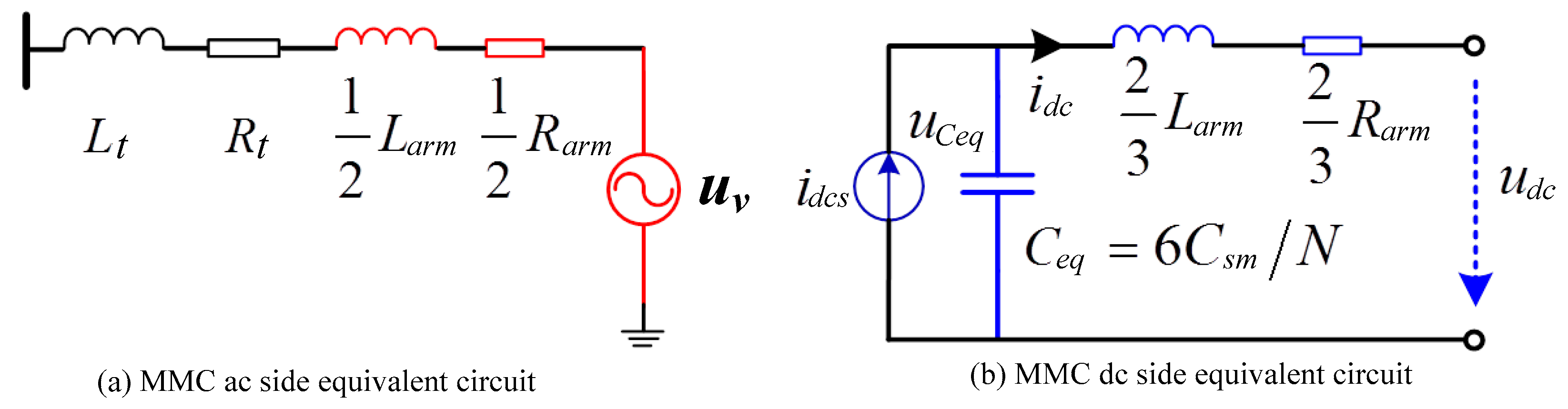
On the basis of (5), (6), and (8), the DC side model of MMC could be derived as in (9):

$$C_{eq}\frac{d{u}_{Ceq}}{dt}={\displaystyle \sum _{j=a,b,c}{u}_{vj}{i}_{vj}}/u_{Ceq}-i_{dc}=i_{dcs}-i_{dc}$$

(9)

where C_eq = 6C_sm/N. Therefore, the AC and DC side model of MMC could be respectively described as in (3), (5), and (9). The equivalent circuit of MMC is plotted in Figure 2, where u_v is the phasor of the three-phase voltage u_vj (j = a, b, c).

3. Deduction of Small-Signal Model for Modular Multilevel Converter Based High-Voltage Direct Current (MMC-HVDC)

3.1. Structure of Small-Signal Model

The dq-frame vector current controller is widely used in practical MMC-HVDCs. With the dq-frame vector current controller, the MMC AC voltage is generated by the inner controller, and the current orders to the inner controller are calculated from the outer controller [22]. The small-signal model for determine minimum SCR is derived based on the AC and DC side equivalent circuit that is illustrated in Section 2. As plotted in Figure 3, the dq-frame vector current controller, the MMC AC side equivalent circuit and the connected AC system could be modeled as a subsystem while the MMC DC side equivalent circuit and the DC network could be modeled as another subsystem. The basic structure of a small-signal model for an m-terminal MMC-HVDC is plotted in Figure 3.

Here in Figure 3, u_s, L_s and R_s are the equivalent voltage source phasor, the equivalent inductor, and the equivalent resistor of the connected AC system, respectively. P_g and Q_g is the active and reactive power injecting into the MMC; P_v and Q_v are the active and reactive power injecting into the voltage source u_v; u_g and i_v denote the phasor of the three-phase voltage u_gj and the three-phase current i_vj (j = a, b, c); L and R are the connecting reactor and resistor between PCC and u_v, which could be calculated according to Figure 2a:

$$\{\begin{array}{c}L=L_t+0.5L_{arm}\\ R=R_t+0.5R_{arm}\end{array}$$

(10)

3.2. Small-Signal Model of MMC Subsystem

3.2.1. Small-Signal Model of Inner Controller and MMC AC Side Model

According to (3), the dq-frame mathematical model of MMC AC side could be deduced as in (11):

$$L\frac{d}{dt}\left[\begin{array}{c}{i}_{vd}\\ i_{vq}\end{array}\right]=\left[\begin{array}{c}{u}_{gd}\\ u_{gq}\end{array}\right]-\left[\begin{array}{c}{u}_{vd}\\ u_{vq}\end{array}\right]+\left[\begin{array}{c}-R{\omega }_{g}L\\ -{\omega }_{g}L-R\end{array}\right]\left[\begin{array}{c}{i}_{vd}\\ i_{vq}\end{array}\right]$$

(11)

The block diagram of the MMC AC side model together with the inner controller is plotted in Figure 4.

Here in Figure 4, i_vd and i_vq are the d-axis and the q-axis component of i_v; i_vdref and i_vqref are the reference values of i_vd and i_vq; u_gd and u_gq are the d-axis and the q-axis component of u_g; uvd and uvq are the d-axis and the q-axis component of u_v; u_vdref and u_vqref are the reference value of u_vd and u_vq; K_pd (K_pq) and K_id (K_iq) are the proportional gain and the integral gain of the inner controller d-axis (q-axis); ω_g is the instantaneous fundamental angular speed; Considering the small time-delay of modulation process, u_vdref (u_vqref) is supposed the same as u_vd (u_vq) in this paper.

In deducing the small-signal model, the prefix Δ and subscript 0 mean the small deviation and initial value of each variable. Based on the block diagram in Figure 4, the small-signal model of the MMC AC side model together with the inner controller could be derived as (12).

$$\{\begin{array}{l}\frac{d\Delta i_{vd}}{dt}=-\frac{R}{L}\Delta i_{vd}+\frac{K_{pd}}{L}\left(\Delta i_{vdref}-\Delta i_{vd}\right)+\frac{1}{L}\Delta M_{id}\\ \frac{d\Delta i_{vq}}{dt}=-\frac{R}{L}\Delta i_{vq}+\frac{K_{pq}}{L}\left(\Delta i_{vqref}-\Delta i_{vq}\right)+\frac{1}{L}\Delta M_{iq}\\ \frac{d\Delta M_{id}}{dt}=K_{id}\left(\Delta i_{vdref}-\Delta i_{vd}\right)\\ \frac{d\Delta M_{iq}}{dt}=K_{iq}\left(\Delta i_{vqref}-\Delta i_{vq}\right)\end{array}$$

(12)

Here in (12), M_id (M_iq) is the state variable of the inner controller d-axis (q-axis) integral part.

3.2.2. Small-Signal Model of Phase-Locked Loop (PLL)

In this paper, the widely used single synchronous reference frame phase-locked loop (SRF-PLL) [23] is studied, and its block diagram is plotted in Figure 5. As plotted in Figure 5, u_gx and u_gy are the x-axis and y-axis component of u_g in common network frame [24]; K_pθ and K_iθ are the proportional gain and the integral gain of the PI controller; θ_g is the output of PLL.

Suppose M_iθ is the state variable of the integral part in the PI controller of SRF-PLL, the respectively small-signal model of PLL could be expressed as (13):

$$\{\begin{array}{l}\frac{d\Delta M_{i\theta }}{dt}=K_{i\theta }\Delta u_{gq}\\ \frac{d\Delta {\theta }_g}{dt}=\Delta {\omega }_g=K_{p\theta }\Delta u_{gq}+\Delta M_{i\theta }\end{array}$$

(13)

On the basis of Kirchhoff’s voltage law, the dynamics of the AC system and MMC AC side equivalent circuit could be described as (14):

$$\{\begin{array}{l}\frac{d{i}_{vd}}{dt}=\frac{u_{gd}-u_{vd}-R{i}_{vd}+{\omega }_{g}L{i}_{vq}}{L}=\frac{u_{sd}-u_{gd}-R_s{i}_{vd}+{\omega }_g{L}_s{i}_{vq}}{L_s}\\ \frac{d{i}_{vq}}{dt}=\frac{u_{gq}-u_{vq}-R{i}_{vq}-{\omega }_{g}L{i}_{vd}}{L}=\frac{u_{sq}-u_{gq}-R_s{i}_{vq}-{\omega }_g{L}_s{i}_{vd}}{L_s}\end{array}$$

(14)

On the basis of the linearized small-signal model of (14), Δu_gd and Δu_gq could be derived as (15):

$$\{\begin{array}{l}\Delta u_{gd}=\frac{L}{L_s+L}\Delta u_{sd}+\frac{L_s}{L_s+L}\Delta u_{vd}+\frac{R{L}_s-R_{s}L}{L_s+L}\Delta i_{vd}\\ \Delta u_{gq}=\frac{L}{L_s+L}\Delta u_{sq}+\frac{L_s}{L_s+L}\Delta u_{vq}+\frac{R{L}_s-R_{s}L}{L_s+L}\Delta i_{vq}\end{array}$$

(15)

On the basis of Figure 4, the linearized small-signal model of the inner controller could be derived as (16):

$$\{\begin{array}{l}\Delta u_{vd}=\Delta u_{gd}+{\omega }_{g0}L\Delta i_{vq}+L{i}_{vq0}\Delta {\omega }_g-K_{pd}\left(\Delta i_{vdref}-\Delta i_{vd}\right)-\Delta M_{id}\\ \Delta u_{vq}=\Delta u_{gq}-{\omega }_{g0}L\Delta i_{vd}-L{i}_{vd0}\Delta {\omega }_g-K_{pq}\left(\Delta i_{vqref}-\Delta i_{vq}\right)-\Delta M_{iq}\end{array}$$

(16)

Note that the relationship of u_s in the dq-frame and the common network frame as in (17), Δu_sd and Δu_sq could be represented by u_sx0, u_sy0 and Δθ_g as in (18):

$$u_{sd}+j{u}_{sq}=\left(u_{sx}+j{u}_{sy}\right)e^{-j{\theta }_g}$$

(17)

$$\{\begin{array}{l}\Delta u_{sd}=\left(-u_{sx0}\sin {\theta }_{g0}+u_{sy0}\cos {\theta }_{g0}\right)\Delta {\theta }_g=U_{d0}\Delta {\theta }_g\\ \Delta u_{sq}=\left(-u_{sx0}\cos {\theta }_{g0}-u_{sy0}\sin {\theta }_{g0}\right)\Delta {\theta }_g=U_{q0}\Delta {\theta }_g\end{array}$$

(18)

where u_sd and u_sq are the d-axis and the q-axis component of us in the dq-frame; u_sx and u_sy are the x-axis and the y-axis component of us in the common network frame; U_d0 and U_q0 is the intermediate variables.

On the basis of (12)–(18), the small-signal model of the MMC AC side model, the inner controller and the PLL could be derived as (19):

$$\frac{d\Delta x_v^{\prime }}{dt}=A_v^{\prime }\Delta x_v^{\prime }+B_r^{\prime }\Delta r^{\prime }+B_u^{\prime }\Delta u_{Ceq}$$

(19)

where $\Delta x_v^{\prime }={\left[\Delta i_{vd}\Delta i_{vq}\Delta M_{id}\Delta M_{iq}\Delta M_{i\theta }\Delta {\theta }_g\right]}^T$, $\Delta r^{\prime }={\left[\Delta i_{vdref}\Delta i_{vqref}\right]}^T$, $B_{\mathrm{u}}^{\prime }={\left[0\right]}_{6\times 1}$; the detailed expressions of $A_{\mathrm{v}}^{\prime }$ and $B_{\mathrm{r}}^{\prime }$ of which are referred to the Appendix A.

3.2.3. Small-Signal Model of MMC DC Side Current Source

The MMC DC side current source i_dcs could be derived based on the conservation of active power.

$$i_{dcs}=\frac{u_{vd}{i}_{vd}+u_{vq}{i}_{vq}}{u_{Ceq}}$$

(20)

The linearized small-signal model of (20) could be written as (21); (21) could be further simplified into (22) after eliminating Δu_vd and Δu_vq:

$$\Delta i_{dcs}=\frac{u_{vd0}}{u_{Ceq0}}\Delta i_{vd}+\frac{u_{vq0}}{u_{Ceq0}}\Delta i_{vq}+\frac{i_{vd0}}{u_{Ceq0}}\Delta u_{vd}+\frac{i_{vq0}}{u_{Ceq0}}\Delta u_{vq}-\frac{i_{vd0}{u}_{vd0}+i_{vq0}{u}_{vq0}}{u_{Ceq0}^2}\Delta u_{Ceq}$$

(21)

$$\Delta i_{dcs}=C_v^{\prime }\Delta x_v^{\prime }+D_r^{\prime }\Delta r^{\prime }+D_u^{\prime }\Delta u_{Ceq}$$

(22)

where the detailed expressions of $C_v^{\prime }$, $D_r^{\prime }$ and $D_{\mathrm{u}}^{\prime }$ of which are referred to the Appendix A.

$$\{\begin{array}{l}\frac{d\Delta x_v^{\prime }}{dt}=A_v^{\prime }\Delta x_v^{\prime }+B_r^{\prime }\Delta r^{\prime }+B_u^{\prime }\Delta u_{Ceq}\\ \Delta i_{dcs}=C_v^{\prime }\Delta x_v^{\prime }+D_r^{\prime }\Delta r^{\prime }+D_u^{\prime }\Delta u_{Ceq}\end{array}$$

(23)

3.2.4. Small-Signal Model of Outer Controller

Because the current order i_vdref and u_vqref are generated by the outer controller, the small-signal model of MMC subsystem could be deducted by eliminating in (23) with the small-signal model of outer controller.

Theoretically, the d-axis current order i_vdref could be generated by the active power controller or the DC voltage controller; the q-axis current order i_vqref could be generated by the reactive power controller or the AC voltage controller. Therefore, details of the small-signal model of the aforementioned four types of outer controllers can be found in the following paragraphs.

For the DC voltage controller, the small-signal model is outlined as (24), where M_iUdc, K_iUdc, and K_pUdc are the state variable of the integral part, the proportional gain, and the integral gain of the outer controller.

$$\{\begin{array}{l}\frac{d\Delta M_{iUdc}}{dt}=K_{iUdc}\left(\Delta u_{dcref}-\Delta u_{Ceq}\right)\\ \Delta i_{vdref}=K_{pUdc}\left(\Delta u_{dcref}-\Delta u_{Ceq}\right)+\Delta M_{iUdc}\end{array}$$

(24)

For the active power controller, the small-signal model is outlined as (25), where M_iPg, K_iPg, and K_pPg are the state variable of the integral part, the proportional gain, and the integral gain of the outer controller.

$$\{\begin{array}{l}\Delta i_{vdref}=K_{pPg}\left(\Delta P_{gref}-\Delta P_g\right)+\Delta M_{iPg}\\ \frac{d\Delta M_{iPg}}{dt}=K_{iPg}\left(\Delta P_{gref}-\Delta P_g\right)\\ \Delta P_g=u_{gd0}\Delta i_{vd}+u_{gq0}\Delta i_{vq}+i_{vd0}\Delta u_{gd}+i_{vq0}\Delta u_{gq}\end{array}$$

(25)

For the reactive power controller, the small-signal model is outlined as (26), where M_iQg, K_iQg, and K_pQg are the state variable of the integral part, the proportional gain, and the integral gain of the outer controller.

$$\{\begin{array}{l}\Delta i_{vqref}=K_{pQg}\left(-\Delta Q_{gref}+\Delta Q_g\right)+\Delta M_{iQg}\\ \frac{d\Delta M_{iQg}}{dt}=K_{iQg}\left(-\Delta Q_{gref}+\Delta Q_g\right)\\ \Delta Q_g=u_{gq0}\Delta i_{vd}-u_{gd0}\Delta i_{vq}-i_{vq0}\Delta u_{gd}+i_{vd0}\Delta u_{gq}\end{array}$$

(26)

For the AC voltage controller, the small-signal model is outlined as (27), where M_iUac, K_iUac, and K_pUac are the state variable of the integral part, the proportional gain, and the integral gain of the outer controller.

$$\{\begin{array}{l}\frac{d\Delta M_{iUg}}{dt}=K_{iUg}\left(\Delta U_{gref}-\Delta U_g\right)\\ \Delta i_{vqref}=K_{pUg}\left(\Delta U_{gref}-\Delta U_g\right)+\Delta M_{iUg}\\ \Delta U_g=\frac{u_{gd0}\Delta u_{gd}+u_{gq0}\Delta u_{gq}}{\sqrt{u_{gd0}^2+u_{gq0}^2}}\end{array}$$

(27)

After eliminating the intermediate variables such as Δu_gd and Δu_gq in (25)–(27), the small-signal model of MMC subsystem could be derived as (28) by substituting (24)–(27) into (23):

$$\{\begin{array}{l}\frac{d\Delta x_v}{dt}=A_v\Delta x_v+B_r\Delta r+B_u\Delta u_{Ceq}\\ \Delta i_{dcs}=C_v\Delta x_v+D_r\Delta r+D_u\Delta u_{Ceq}\end{array}$$

(28)

where A_v, B_r, B_u, C_v, D_r, and D_u differ with different outer control schemes; the small deviation of state variables Δx_v and the small deviation of outer controller reference value Δr also differ with different outer control schemes. For example, if the MMC controls the DC voltage and the reactive power, Δx_v and Δr could be written as (29):

$$\{\begin{array}{l}\Delta x_v={\left[\Delta i_{vd}\Delta i_{vq}\Delta M_{id}\Delta M_{iq}\Delta M_{i\theta }\Delta {\theta }_g\Delta M_{iUdc}\Delta M_{iQg}\right]}^T\\ \Delta r={\left[\Delta u_{dcref}\Delta Q_{gref}\right]}^T\end{array}$$

(29)

3.3. Small-Signal Model of DC Network

Generally speaking, there are two types of nodes in the DC network of MMC-HVDC, namely the converter station nodes and the interconnection nodes. The converter station nodes are the nodes where the DC network and the converter stations are connected, and the interconnection nodes are the nodes that do not connect to any converter station. Figure 6 outlines the DC network topology of a four-ternimal MMC-HVDC and its incidence matrix T. The element T_ik in T equals 1 (−1) if the current in DC line k flows out of (into) node i; T_ik equals 0 if the current in DC line k does not connect to node i.

For an m-terminal MMC-HVDC with b DC lines and n nodes, the state-space model of the DC network could be generalized as (30) after representing the DC line by its π section model:

$$\{\begin{array}{l}C\frac{du}{dt}=M_E{i}_{dcs}-T_{E}i\\ L\frac{di}{dt}=T_E^{T}u-Ri\end{array}$$

(30)

where $u=\left[\begin{array}{c}{u}_{dc(n\times 1)}\\ u_{Ceq(m\times 1)}\end{array}\right]$, $i=\left[\begin{array}{c}{i}_{br(b\times 1)}\\ i_{dc(m\times 1)}\end{array}\right]$, $T_E=\left[\begin{array}{cc}{T}_{(n\times b)}& -M_{(n\times m)}\\ 0_{(m\times b)}& I_{(m\times m)}\end{array}\right]$, $M_{(n\times m)}=\left[\begin{array}{c}{I}_{(m\times m)}\\ 0_{(n-m)\times m}\end{array}\right]$, $M_E=\left[\begin{array}{c}{0}_{(m\times m)}\\ M_{(n\times m)}\end{array}\right]$, $C=diag\left[\begin{array}{c}{C}_{br\Sigma (n\times 1)}\\ C_{eq(m\times 1)}\end{array}\right]$, $L=diag\left[\begin{array}{c}{L}_{br(b\times 1)}\\ L_{eq(m\times 1)}\end{array}\right]$, $R=diag\left[\begin{array}{c}{R}_{br(b\times 1)}\\ R_{eq(m\times 1)}\end{array}\right]$; C_brΣ = |T|C_br, where C_br = [C_br1, …, C_brb]^T is the vector of DC line capacitors; i_br = [i_br1, …, i_brb]^T is the vector of DC line currents; u_dc = [u_dc1, …, u_dcn]^T is the vector of DC node voltages; i_dc = [i_dc1, …, i_dcm]^T is the vector of injection currents at converter station nodes; L_br = [L_br1, …, L_brb]^T is the vector of DC line inductors; R_br = [R_br1, …, R_brb]^T is the vector of DC line resistors; i_dcs = [i_dcs1, …, i_dcsm]^T is the vector of controlled current source of MMCs; u_Ceq = [u_Ceq1, …, u_Ceqm]^T is the vector of DC node voltages; C_eq = [C_eq1, …, C_eqm]^T is the vector of MMC equivalent capacitors; L_eq = [2/3L_arm1 + L_dc1, …, 2/3L_armm + L_dcm]^T is the vector of the MMC DC side equivalent inductors; R_eq = [2/3R_arm1, …, 2/3R_armm]^T is the vector of the MMC dc side equivalent resistors. I is the identical matrix; 0 is the zero matrix; diag[V] is the diagonal matrix whose i-th non zero element equals to the i-th element of vector V.

The linearized small-signal model of (30) could be derived as (31):

$$\{\begin{array}{l}\frac{d\Delta x_G}{dt}=A_G\Delta x_G+B_G\Delta i_{dcs}\\ \Delta u_{Ceq}=C_G\Delta x_G\end{array}$$

(31)

where $\Delta x_G=\left[\begin{array}{c}\Delta u_{(n+m)\times 1}\\ \Delta i_{(b+m)\times 1}\end{array}\right]$, $A_G=\left[\begin{array}{cc}{0}_{(n+m)\times (n+m)}& -C^{-1}{T}_E\\ L^{-1}{T}_E^T& -L^{-1}R\end{array}\right]$, $B_G=\left[\begin{array}{c}{C}^{-1}{M}_E\\ 0_{(b+m)\times m}\end{array}\right]$, $C_G=\left[\begin{array}{ccc}{0}_{(m\times n)}& I_{(m\times m)}& 0_{m\times (b+m)}\end{array}\right]$.

3.4. Small-Signal Model of MMC-HVDC

According to Section 3.1, small-signal model of each MMC subsystem could be described as (28). For an m-terminal MMC-HVDC, all the m MMC subsystems could be modeled as follows:

$$\{\begin{array}{l}\frac{d\Delta x_{MMC}}{dt}=A_{MMC}\Delta x_{MMC}+B_{MMCr}\Delta r_{ref}+B_{MMCu}\Delta u_{Ceq}\\ \Delta i_{dcs}=C_{MMC}\Delta x_{MMC}+D_{MMCr}\Delta r_{ref}+D_{MMCu}\Delta u_{Ceq}\end{array}$$

(32)

where $\Delta x_{MMC}=\left[\begin{array}{c}\Delta x_{v1}\\ ⋮\\ \Delta x_{vm}\end{array}\right]$, $\Delta r_{ref}=\left[\begin{array}{c}\Delta r_1\\ ⋮\\ \Delta r_m\end{array}\right]$, $A_{MMC}=diag\left[\begin{array}{c}{A}_{v1}\\ ⋮\\ A_{vm}\end{array}\right]$, $B_{MMCr}=diag\left[\begin{array}{c}{B}_{r1}\\ ⋮\\ B_{rm}\end{array}\right]$, $B_{MMCu}=diag\left[\begin{array}{c}{B}_{u1}\\ ⋮\\ B_{um}\end{array}\right]$, $C_{MMC}=diag\left[\begin{array}{c}{C}_{v1}\\ ⋮\\ C_{vm}\end{array}\right]$, $D_{MMCr}=diag\left[\begin{array}{c}{D}_{r1}\\ ⋮\\ D_{rm}\end{array}\right]$, $D_{MMCu}=diag\left[\begin{array}{c}{D}_{u1}\\ M\\ D_{um}\end{array}\right]$.

The linearized small-signal model of the whole MMC-HVDC could be derived after merging (31) and (32):

$$\frac{d\Delta x_{sys}}{dt}=A_{sys}\Delta x_{sys}+B_{sys}\Delta r_{ref}$$

(33)

where $\Delta x_{sys}=\left[\begin{array}{c}\Delta x_{MMC}\\ \Delta x_G\end{array}\right]$, $A_{sys}=\left[\begin{array}{cc}{A}_{MMC}& B_{MMCu}{C}_G\\ B_G{C}_{MMC}& A_G+B_G{D}_{MMCu}{C}_G\end{array}\right]$, $B_{sys}=\left[\begin{array}{c}{B}_{MMCr}\\ B_G{D}_{MMCr}\end{array}\right]$.

On the basis of the eigenvalues of matrix A_sys, the minimum SCR for MMC-HVDC could be determined considering the small-signal stability.

4. Procedure for Determining Minimum Short Circuit Radio (SCR) Based on Small-Signal Stability Analysis

4.1. Determining Steady-State Power Flow of MMC-HVDC

From the process of linearization in Section 3, it is known that matrix A_sys is associated with the initial steady-state operation point. During planning stages, the operations of power systems under rated conditions are of prime concern. Therefore, the rated operation point of the MMC-HVDC system with active power and reactive power set as 1.0 pu and 0.0 pu is considered in this paper. According to the aforementioned analysis, the initial value of the state-variables x_sys could be calculated directly when the power flow of MMC-HVDC is determined. Therefore, the procedure for determining the power flow of MMC-HVDC is described in this section, which contains four steps:

Step 1. Calculate the steady-state power flow of the MMC subsystem that controls the active power with the Newton-Raphson method. The steady-state power flow of MMC subsystem satisfies (34), where subscript 0 means the steady-state initial values of each variable. For the MMC station that controls the active power, the known variables in (34) are P_g0 (1.0 pu for rectifier and −1.0 pu for inverter), Q_g0 (0.0 pu), U_g0 (1.0 pu), and u_sy0 (0.0 pu). After solving (34), θ_g0 equals arctan(u_gy0/u_gx0).

$$\{\begin{array}{l}{P}_{g0}=u_{gx0}{i}_{vx0}+u_{gy0}{i}_{vy0}\\ Q_{g0}=-u_{gx0}{i}_{vy0}+u_{gy0}{i}_{vx0}\\ P_{v0}=u_{vx0}{i}_{vx0}+u_{vy0}{i}_{vy0}\\ Q_{v0}=-u_{vx0}{i}_{vy0}+u_{vy0}{i}_{vx0}\\ u_{vx0}=u_{sx0}-\left(R+R_s\right)i_{vx0}+{\omega }_{g0}\left(L+L_s\right)i_{vy0}\\ u_{vy0}=u_{sy0}-\left(R+R_s\right)i_{vy0}-{\omega }_{g0}\left(L+L_s\right)i_{vx0}\\ u_{gx0}=u_{sx0}-R_s{i}_{vx0}+{\omega }_{g0}{L}_s{i}_{vy0}\\ u_{gy0}=u_{sy0}-R_s{i}_{vy0}-{\omega }_{g0}{L}_s{i}_{vx0}\\ U_{g0}=\sqrt{u_{gx0}^2+u_{gy0}^2}\end{array}$$

(34)

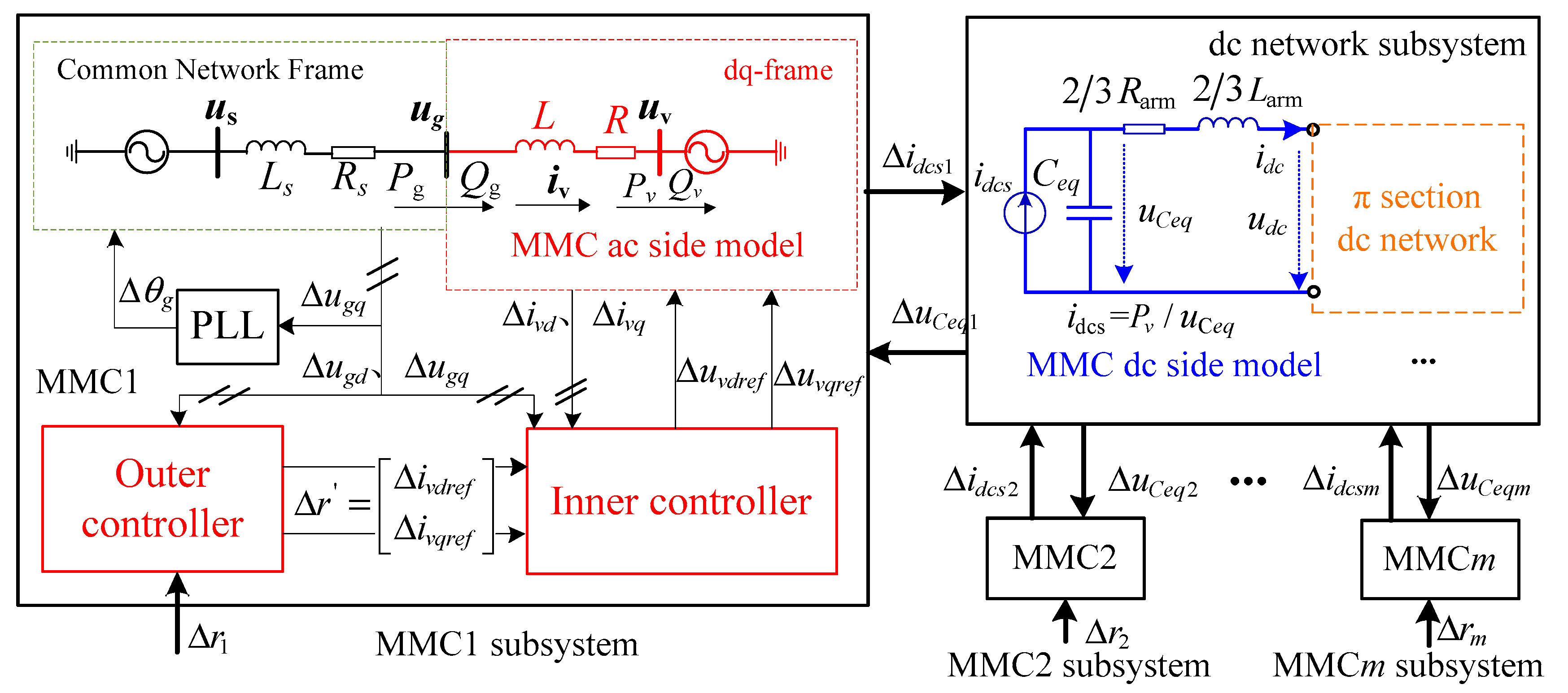
Step 2: Calculating the steady-state power flow of the DC net subsystem by setting the DC voltage as 1.0 pu for the MMC that controls the DC voltage and the DC power, supplied by current source i_dcs as seen in Figure 3, as P_v0 for the MMC that controls the active power.

Step 3: Calculate the steady-state power flow of the MMC subsystem that controls the DC voltage described by (34) with the Newton–Raphson method. For the MMC station that controls the DC voltage, the known variables in (34) are P_v0 (already calculated in Step 2), Q_g0 (0.0 pu), U_g0 (1.0 pu) and u_sy0 (0.0 pu). After solving (34), θ_g0 equals arctan(u_gy0/u_gx0).

Step 4: Transform the calculated results from the common network frame to the dq-frame with θ_g0 for concerned MMC subsystems.

In most studies that use small-signal analysis, the magnitude of u_s were supposed as a constant (usually around 1.0 pu) to determine the initial values of the state variables. However, for AC systems with small SCR, there would be a great deviation between the calculated voltage and the rated voltage at the point of common coupling (PCC) with the above assumption, and it would eventually affect the rationality of the small-signal analysis results. In accordance with LCC-HVDC, the PCC voltage is set as its rated value [25].

4.2. Procedure for Determining Minimum SCR

Procedures to determine the minimum SCR requirement of MMC-HVDC and a possible framework are described as follows:

Step 1. To calculate matrix A_sys, the reference value r_ref, the parameters of PI controllers, and the SCR should first be specified. After selecting an initial SCR, repeat Steps 2–4.

Step 2. Calculate the MMC AC side power flow with the Newton–Raphson method. Then, calculate the initial values of the state-variables x_sys based on the calculated power flow results. Derive the linearized small-signal model of the whole MMC-HVDC as described in Section 3, and determine the matrix A_sys.

Step 3. Calculate the eigenvalues of matrix A_sys; the small-signal stability constraint is satisfied at the specified SCR if the real part of all the eigenvalues is negative. If the small-signal stability constraint is not satisfied, stop calculation and output the smallest SCR that satisfied the small-signal stability constraint.

Step 4. If small-signal stability constraint in Step 3 is satisfied, check whether the Thevenin equivalent voltage of the AC system u_s is within the safety limit. In this paper, u_s satisfies the voltage safety limit constraint, if the magnitude of u_s is between 0.9 pu and 1.2 pu If u_s satisfies the voltage safety limit constraint, decrease the SCR by increasing the AC system impedance and go back to Step 2. Otherwise, stop calculation and output the smallest SCR that satisfied the safety limit constraint.

The respectively flowchart of the proposed procedure is outlined in Figure 7.

5. Case Study

5.1. System Parameters

The case studies are carried out based on a two-terminal MMC-HVDC, as plotted in Figure 8. To give general conclusions, the actual value and the nominalized value of the main parameters in the test system are listed in

Table 1. Main Circuit Parameters of Test System.

Item	Actual Values	Nominalized Values
AC system rated voltage	220 kV	1.0 pu
Transformer ratio	220 kV/210 kV	/
Transformer rated capacity	480 MVA	1.2 pu
Transformer leakage inductance	32.1 mH	0.0833 pu
Transformer resistor	0.605 Ω	0.005 pu
Rated dc voltage	400 kV	1.0 pu
MMC rated capacity	400 MVA	1.0 pu
MMC arm reactor	76 mH	0.197 pu
MMC arm resistor	0.48 Ω	0.004 pu
Number of SMs per arm	200	/
MMC SM capacitor	6667 μF	25.13 pu
Smoothing reactor	100 mH	0.0785 pu
DC line resistor	1.3 Ω	0.00325 pu
DC line reactor	82.7 mH	0.0649 pu
DC line capacitor	0.7 μF	0.0879 pu

. The parameters in Table 1 approximate the two-terminal test system in [26]. For the voltages at the secondary side of the converter transformer, the base value is chosen as the rated voltage of the transformer secondary side; at the transformer primary side, the voltage base value is selected as the rated voltage at this side. The base value of DC side voltage is the rated DC voltage. The base power is supposed as the rated capacity of the MMC.

The parameters of PI controllers are listed in

Table 2. Parameters of Proportional-Integral (PI) Controllers in Test System.

Parameters of PI Controller	Proportional Gain/Pu	Integral Gain/Pu
D-axis of inner controller	0.0032	0.048
Q-axis of inner controller	0.0032	0.048
PLL	1.414	1.000
DC voltage controller	2.513	0.126
Active power controller	0.050	0.160
Reactive power controller	0.050	0.106
AC voltage controller	0.050	0.160

. The initial SCR of the sending system and the receiving system are both set as 3.0. The AC system impedance angle was supposed to be 80°, 82°, 86°, and 90°. The subscript 1 represents the variables in the rectifier MMC, and the subscript 2 represents the variables in the inverter MMC. The following four control schemes are listed in

Table 3. Studied Control Schemes for MMC-HVDC.

Control Scheme	Rectifier MMC	Inverter MMC
1	active power + reactive power	dc voltage + reactive power
2	dc voltage + reactive power	active power + reactive power
3	active power + ac voltage	dc voltage + ac voltage
4	dc voltage + ac voltage	active power + ac voltage

, where the reference value of DC voltage, active power, reactive power and AC voltage are set as 1.0 pu, 1.0 pu, 0.0 pu, and 1.0 pu, respectively. The reference direction of active power is from the rectifier to the inverter.

5.2. Validation Results

5.2.1. Small-Signal Stability Analysis

The validation is performed based on Control Scheme 1, the minimum SCR was studied on the assumption that the AC system impedance angle was 80°. Suppose the SCR decreases from 3.0 to 1.0 with a step of 0.01, the root locus was plotted in Figure 9 based on the procedure in Section 4.

When SCR decreases to 1.95, the calculated eigenvalues of matrix A_sys are listed in

Table 4. Calculated Eigenvalues of MMC-HVDC with Sending End of SCR = 1.95.

No.	Eigenvalue	No.	Eigenvalue
1, 2	−0.0183 ± j25.223	12, 13	−2.502 ± j1.210
3, 4	−0.0101 ± j16.932	14, 15	−0.194 ± j0.764
5	−15.140	16, 17	−0.615 ± j0.509
6	−15.140	18, 19	−0.644 ± j0.118
7	−15.140	20	−0.036
8	−15.140	21	−0.112
9	−4.115	22	−0.099
10	−3.970	23	−0.101
11	−4.029

. It could be concluded that the small-signal stability is satisfied. However, the equivalent voltage source of the sending system is 1.2006 pu, which exceeds the voltage safety limit. Therefore, the active power of the rectifier could not reach 1.0 pu if SCR of sending system is lower than 1.95. The equivalent voltage source of receiving system is 1.036 pu, which is within the voltage safety limit.

Then, decrease the SCR of the receiving system while maintaining the SCR of the sending system as 1.95; the system will be unstable when the SCR of the receiving system decreases to 1.36 or less. The calculated eigenvalues of matrix A_sys, the state variable with the participation factor of the largest absolute value (denoted as ‘SVLPF’) and the respective participation factor (denoted as ‘LPF’) are listed in

Table 5. Calculated Eigenvalues of MMC-HVDC with Receiving End of SCR = 1.36.

No.	Eigenvalue	SVLPF	LPF	No.	Eigenvalue	SVLPF	LPF
1	−59.133	θg2	2.550	13	−3.622	Miq2	0.760
2, 3	−0.0183 ± j25.223	ibr1	0.275 ± j0.001	14, 15	−0.103 ± j0.873	uCeq2	0.504 ± j0.023
4, 5	−0.0101 ± j16.932	idc1, idc2	0.250	16, 17	−0.615 ± j0.510	θg1	0.507 ± j0.321
6	−15.140	ivd1	1.378	18	−0.581	uCeq2	−2.693
7	−15.140	ivq1	1.382	19	−0.365	uCeq2	2.703
8	−15.140	ivd2	1.134	20	−0.113	MiPg1	0.635
9	−15.140	ivq2	1.404	21	−0.099	MiQg1	0.566
10	−5.287	Mid2	0.794	22	−0.038	MiUdc2	1.214
11	−4.115	Miq1	1.222	23	0.007	MiQg2	1.029
12	−4.029	Mid1	1.212

.

According to Table 5, when SCR decreases, the first eigenvalue whose real part become larger than 0 is the 23-th eigenvalue, and state variable with the participation factor of the largest absolute value is M_iQg2. Therefore, the 23-th eigenvalue as well as the minimum SCR is mainly influenced by M_iQg2. Because M_iQg2 is in direct proportion to K_iQg2, it could be concluded that the 23-th eigenvalue is mainly influenced by K_iQg2. Theoretically, the minimum SCR is most sensitive to parameter K_iQg2.

Next, the robustness analysis on the procedure is conducted by changing K_iQg2 from half its original value to two times its original value (0.053–0.212). The calculated minimum SCR requirement of the receiving end, together with the 23-th eigenvalue, is plotted in Figure 10. The results show that the calculated minimum SCR remains unchanged with the decrease step of 0.01, although the 23-th eigenvalue changes a little with the variation of K_iQg2. The robustness of the procedure is proved.

5.2.2. Time-Domain Validation

The time-domain validation was performed on PSCAD/EMTDC. The simulation results of the minimum sending end SCR and the minimum receiving end SCR are plotted in Figure 11 and Figure 12.

As seen in Figure 11 and Figure 12, U_{crj_av} is average SM capacitor voltage, where j (j = a, b, c) denotes phase and r (r = p, n) denotes the upper or lower arm.

As seen in Figure 11, the rectifier MMC could not transmit 1.0 pu active power if the SCR decrease from 1.95 to 1.91. When SCR is less than 1.95, the AC system equivalent voltage source is limited to the voltage safety limit (1.2 pu), and the decrease would cause the voltage drop at PCC. In consideration of the current constraint [13], the active power of rectifier would inevitably decrease. The relevant MMC-HVDC could operate stably under this circumstance. The simulation results are consistent with the analytical results, and prove that the rectifier could not transmit 1.0 pu active power with an SCR lower than 1.95 when considering the voltage safety limit constraint.

As seen in Figure 12, the MMC-HVDC could not operate stably if the SCR of the receiving system decreases from 1.37 to 1.32. The simulation results are consistent with the analytical results by small-signal analysis and demonstrate that the MMC-HVDC could not operate stably with an SCR lower than 1.36 when transmitting 1.0 pu active power.

Although certain errors exist between the simulation results and the analytical results, the error is relatively small enough and is acceptable. Therefore, the validity of the proposed procedure to determine the minimum SCR is proved.

5.3. Minimum SCR Requirement of Four Control Schemes

5.3.1. Control Scheme 1

According to the aforementioned method, the minimum SCR requirement of Control Scheme 1 is calculated and listed in

Table 6. Minimum SCR Requirement of Control Scheme 1.

Impedance Angle/°	Rectifier		Inverter
	Minimum SCR	Restraint Factor	Minimum SCR	Restraint Factor
80	1.95	VSLC	1.36	MiQg2
82	1.85	VSLC	1.37	MiQg2
86	1.67	VSLC	1.38	MiQg2
90	1.51	VSLC	1.46	VSLC

. The restraint factors for transmitting 1.0 pu active power includes the voltage safety limit constraint (denoted as ‘VSLC’) and the state-variables with the largest participate factor for the unstable mode.

According to Table 6, it can be concluded that:

(1)

The calculated minimum SCR is concerned with MMC operation mode and the AC system impedance angle. For the rectifier MMC, the minimum SCR varies 1.51–1.95, and the increase of the AC system impedance angle would make the minimum SCR decrease. For the inverter MMC, the minimum SCR varies 1.36–1.46, and the increase of the AC system impedance angle would make the minimum SCR increase.

(2)

The minimum SCR requirement for the rectifier is larger than for the inverter, which means that the SCR requirement for the connected AC system is stricter for the rectifier MMC.

(3)

For transmitting 1.0 pu active power, the restraint factor for rectifier is the voltage safety limit constraint while the restraint factor for the inverter is mainly the outer reactive power controller.

5.3.2. Control Scheme 2

The minimum SCR requirement of Control scheme 2 is calculated and listed in

Table 7. Minimum SCR Requirement of Control Scheme 2.

Impedance Angle/°	Rectifier		Inverter
	Minimum SCR	Restraint Factor	Minimum SCR	Restraint Factor
80	1.95	VSLC	1.40	MiQg2
82	1.85	VSLC	1.41	MiQg2
86	1.67	VSLC	1.42	MiQg2
90	1.51	VSLC	1.51	VSLC

, and it can be concluded that:

(1)

The calculated minimum SCR is concerned with MMC operation mode and the AC system impedance angle. For the rectifier MMC, the minimum SCR varies 1.51–1.95, and the increase of AC system impedance angle would make the minimum SCR decrease. For the inverter MMC, the minimum SCR varies 1.51–1.40, and the increase of AC system impedance angle would make the minimum SCR increase.

(2)

The minimum SCR requirement for the rectifier is larger than that for the inverter, indicating that the SCR requirement for the connected AC system is stricter for the rectifier MMC.

(3)

For transmitting 1.0 pu active power, the restraint factor for rectifier is the voltage safety limit constraint; in contrast, the restraint factor for the inverter is mainly the outer reactive power controller.

5.3.3. Control Scheme 3

The minimum SCR requirement of Control Scheme 3 is calculated and listed in

Table 8. Minimum SCR Requirement of Control Scheme 3.

Impedance Angle/°	Rectifier		Inverter
	Minimum SCR	Restraint Factor	Minimum SCR	Restraint Factor
80	1.95	VSLC	1.34	Miθ2, θg2
82	1.85	VSLC	1.35	Miθ2, θg2
86	1.67	VSLC	1.36	Miθ2, θg2
90	1.51	VSLC	1.46	VSLC

, and it can be concluded that:

(1)

The calculated minimum SCR is concerned with MMC operation mode and the AC system impedance angle. For the rectifier MMC, the minimum SCR varies 1.51–1.95, and the increase of AC system impedance angle would make the minimum SCR decrease. For the inverter MMC, the minimum SCR varies 1.46–1.34, and the increase of the AC system impedance angle would make the minimum SCR increase.

(2)

The minimum SCR requirement for the rectifier is larger than that for the inverter, indicating that the SCR requirement for the connected AC system is stricter for the rectifier MMC.

(3)

For transmitting 1.0 pu active power, the restraint factor for rectifier is the voltage safety limit constraint; however, the restraint factor for the inverter is mainly the PLL.

5.3.4. Control Scheme 4

The minimum SCR requirement of Control scheme 4 is calculated and listed in

Table 9. Minimum SCR Requirement of Control Scheme 4.

Impedance Angle/°	Rectifier		Inverter
	Minimum SCR	Restraint Factor	Minimum SCR	Restraint Factor
80	1.95	VSLC	1.39	MiQg2
82	1.85	VSLC	1.40	MiQg2
86	1.67	VSLC	1.41	MiQg2
90	1.51	VSLC	1.51	VSLC

, and it can be concluded that:

(1)

The calculated minimum SCR is concerned with MMC operation mode and the AC system impedance angle. For the rectifier MMC, the minimum SCR varies 1.51–1.95, and the increase of AC system impedance angle would make the minimum SCR decrease. For the inverter MMC, the minimum SCR varies 1.51–1.39, and the increase of AC system impedance angle would make the minimum SCR increase.

(2)

The minimum SCR requirement for the rectifier is larger than that for the inverter, indicating that the SCR requirement for the connected AC system is stricter for the rectifier MMC.

(3)

For transmitting 1.0 pu active power, the restraint factors for the rectifier are the voltage safety limit constraint; however, the restraint factor for the inverter is mainly the PLL.

5.3.5. Comparison of Different Minimum SCR Requirements

On the basis of the calculation results listed in Table 6, Table 7, Table 8 and Table 9, it can be concluded that:

(1)

For transmitting 1.0 pu active power, the minimum SCR requirement for rectifier varies 1.51–1.95, and the increase of AC system impedance angle would make the minimum SCR decrease. The minimum SCR requirement of rectifier has nothing to do with the control scheme of rectifier MMC.

(2)

For transmitting 1.0 pu active power, the minimum SCR requirement for inverter varies 1.34–1.51, and the increase of AC system impedance angle would make the minimum SCR increase. The minimum SCR requirement is the largest when the inverter MMC controls the active power and the reactive power. The minimum SCR requirement is the lowest when the inverter MMC controls the DC and the AC voltage.

(3)

The minimum SCR requirement is higher for the rectifier MMC than for the inverter MMC. The restraint factor for the rectifier MMC is voltage safety limit constraint while the restraint factors for inverter are mainly the PLL or the outer reactive power controller.

(4)

The MMC-HVDC could keep operating stably if the SCR of the sending system is slightly lower than the minimum SCR requirement. The MMC-HVDC could not operate stably if the SCR of receiving system is slightly lower than the minimum SCR requirement.

6. Conclusions

On the basis of a small-signal stability analysis, the minimum SCR requirement for MMC-HVDC system is studied in this paper. The results show that the restraint factors for the rectifier MMC is mostly the voltage safety limit constraint, and the minimum SCR requirement of the sending system has nothing to do with the control scheme of rectifier MMC. The restraint factors for inverter MMC is mainly the PLL or the outer reactive power controller; the minimum SCR requirement is the lowest when the inverter MMC controls the DC and AC voltage. The minimum SCR requirement for the connected AC system is stricter for the rectifier; the minimum SCR requirements for the sending and the receiving systems are suggested to be 2.0 and 1.5 in the planning stage. Note that the concerned MMC-HVDC consists of half bridge SMs and adopts vector current control scheme. Future research on this topic could focus on the minimum SCR requirement for MMC-HVDC with full bridge SMs and minimum SCR requirement for MMC-HVDC with other control schemes such as the virtual synchronous generator control scheme or the power synchronization control scheme.

References

1. Eriksson, K. Operational Experience of HVDC Light/TM. In Proceedings of the Seventh International Conference on AC-DC Power Transmission, London, UK, 28–30 November 2001; pp. 205–210. [Google Scholar]
2. Friedrich, K. Modern HVDC PLUS application of VSC in Modular Multilevel Converter topology. IEEE Int. Symp. Ind. Electron. 2010, 3807–3810. [Google Scholar]
3. Peralta, J.; Saad, H.; Dennetiere, S.; Mahseredjian, J.; Nguefeu, S. Detailed and Averaged Models for a 401-Level MMC-HVDC System. IEEE Trans. Power Deliv. 2012, 27, 1501–1508. [Google Scholar] [CrossRef]
4. Allebrod, S.; Hamerski, R.; Marquardt, R. New Transformerless, Scalable Modular Multilevel Converters for HVDC-Transmission. In Proceedings of the IEEE Power Electronics Specialists Conference, Rhodes, Greece, 15–19 June 2008; pp. 174–179. [Google Scholar]
5. Zhang, G.; Xu, Z.; Liu, H. Supply Passive Networks with VSC-HVDC. In Proceedings of the Power Engineering Society Summer Meeting, Vancouver, BC, Canada, 15–19 July 2001. [Google Scholar]
6. Dong, H.; Xu, Z.; Song, P. Optimized Power Redistribution of Offshore Wind Farms Integrated VSC-MTDC Transmissions after Onshore Converter Outage. IEEE Trans. Ind. Electron. 2016, 64, 8948–8958. [Google Scholar]
7. Tang, G.; Xu, Z.; Dong, H. Sliding Mode Robust Control Based Active-Power Modulation of Multi-Terminal HVDC Transmissions. IEEE Trans. Power Syst. 2015, 31, 1614–1623. [Google Scholar] [CrossRef]
8. IEEE. IEEE Guide for Planning DC Links Terminating at AC Locations Having Low Short-Circuit Capacities; IEEE press: Piscataway, NJ, USA, 1997. [Google Scholar]
9. CIGRE WG 14.07. IEEE WG 15.05. Guide for Planning DC Links Terminating at AC Locations Having Low Short-Circuit Capacities, Part 1: AC/DC Interaction Phenomena; CIGRE: Paris, France, 1992. [Google Scholar]
10. Liu, S.; Xu, Z. Study on stable operating region of VSC-HVDC connected to weak AC systems. Proc. CSEEE 2016, 36, 133–144. (In Chinese) [Google Scholar]
11. Zhou, J.; Gole, A. VSC Transmission Limitations Imposed by Ac System Strength and Ac Impedance Characteristics. In Proceedings of the 10th IET International Conference on ac and DC Power Transmission, Birmingham, UK, 4–5 December 2012. [Google Scholar]
12. Zhou, J.; Gole, A. Rationalization of DC Power Transfer Limits for VSC Transmission. In Proceedings of the 11th IET International Conference on ac and DC Power Transmission, Birmingham, UK, 10–12 February 2015. [Google Scholar]
13. Zhang, Z.; Xu, Z.; Jiang, W.; Bie, X. Operating Area for Modular Multilevel Converter Based High-Voltage Direct Current Systems. Proc. IET Renew. Power Gener. 2016, 10, 776–787. [Google Scholar] [CrossRef]
14. Durrant, M.; Werner, H.; Abbott, K. Model of a VSC HVDC Terminal Attached to a Weak AC System. In Proceedings of the 2003 IEEE Conference on Control Applications, Istanbul, Turkey, 25 June 2003; pp. 178–182. [Google Scholar]
15. Zhou, J.; Ding, H.; Fan, S. Impact of short-circuit ratio and phase-locked-loop parameters on the small-signal behavior of a VSC-HVDC converter. IEEE Trans. Power Deliv. 2014, 29, 2287–2296. [Google Scholar] [CrossRef]
16. Yuan, B.; Li, T.; Xu, J.; Yuan, Y.; Zhao, C.; Zhang, F. Small-signal Stability Analysis of Modular Multilevel Converter Connected to a Weak AC System. Proc. CSEE 2017, 37, 5339–5349. (In Chinese) [Google Scholar]
17. Guo, C.; Yin, Z.; Zhao, C. Comparative Study on Small-signal Stability of MMC-HVDC System under Rectification and Inversion Modes. Proc. CSEE 2018, 38, 7349–7358. (In Chinese) [Google Scholar]
18. Ding, H.; Fan, S.; Zhou, J. Parametric Analysis of the Stability of VSC-HVDC Converters. In Proceedings of the 11th IET International Conference on AC and DC Power Transmission, Birmingham, UK, 10–12 February 2015; pp. 1–6. [Google Scholar]
19. Lu, S.; Xu, Z.; Xiao, L. Evaluation and enhancement of control strategies for VSC stations under weak grid strengths. IEEE Trans. Power Syst. 2017, 33, 1836–1847. [Google Scholar] [CrossRef]
20. Jamshidifar, A.; Jovcic, D. Small Signal Dynamic DQ Model of Modular Multilevel Converter for System Studies. In Proceedings of the 2016 IEEE Power and Energy Society General Meeting, Boston, MA, USA, 17–21 July 2016. [Google Scholar]
21. Song, Q.; Liu, W.; Li, X. A Steady-State Analysis Method for a Modular Multilevel Converter. IEEE Trans. Power Electron. 2013, 28, 3702–3713. [Google Scholar] [CrossRef]
22. Guan, M.; Xu, Z. Modeling and Control of a Modular Multilevel Converter-Based HVDC System Under Unbalanced Grid Conditions. IEEE Trans. Power Electron. 2012, 27, 4858–4867. [Google Scholar] [CrossRef]
23. Kaura, V.; Blasko, V. Operation of a phase locked loop system under distorted utility conditions. IEEE Trans. Ind. Appl. 1997, 33, 58–63. [Google Scholar] [CrossRef]
24. Kundur, P. Power System Stability and Control; McGraw-Hill: New York, NY, USA, 1994. [Google Scholar]
25. Gole, A.; Zhou, J. Rationalisation and validation of dc power transfer limits for voltage sourced converter based high voltage DC transmission. IET Gener. Transm. Distrib. 2016, 10, 1327–1335. [Google Scholar]
26. Xiao, L.; Xu, Z.; Xiao, H.; Zhang, Z.; Wang, G.; Xu, Y. Electro-mechanical transient modeling of MMC based multi-terminal HVDC system with DC faults considered. Int. J. Electr. Power Energy Syst. 2019, 113, 1002–1013. [Google Scholar] [CrossRef]
Figure 1. Basic structure of modular multilevel converter (MMC).
Energies 12 03283 g001
Figure 2. AC and DC side equivalent circuit of the modular multilevel converter (MMC).
Energies 12 03283 g002
Figure 3. Basic Structure of a small-signal model.
Energies 12 03283 g003
Figure 4. Basic structure of MMC AC side and the inner controller.
Energies 12 03283 g004
Figure 5. Basic structure of phase-locked loop (PLL).
Energies 12 03283 g005
Figure 6. Topology and incidence matrix of DC network.
Energies 12 03283 g006
Figure 7. Flowchart for determining the minimum SCR requirement of MMC-HVDC.
Energies 12 03283 g007
Figure 8. Single-line diagram of the test system.
Energies 12 03283 g008
Figure 9. Root locus of test system with Control Scheme 1.
Energies 12 03283 g009
Figure 10. Minimum SCR and 23-th eigenvalue of test system with different KiQg2.
Energies 12 03283 g010
Figure 11. Simulation results of minimum sending end SCR.
Energies 12 03283 g011
Figure 12. Simulation results of minimum receiving end SCR.
Energies 12 03283 g012