T–S Fuzzy Modeling for Aircraft Engines: The Clustering and Identification Approach

Abstract

This paper presents a data-based Takagi-Sugeno (T–S) fuzzy modeling approach for aircraft engines in the flight envelope. We propose a series of T–S fuzzy models for engines with flight conditions as premises and engine linear dynamic models as consequences. By engine dynamic clustering, we determine rough T–S fuzzy models to approximate the nonlinear dynamics of engines in the flight envelope. After that, the maximum–minimum distance-based fuzzy c-means (MMD-FCM) algorithm comes to refine the fuzzy rules and the least square method (LSM) comes to identify premise parameters for each single rough model. The proposed MMD-FCM algorithm guarantees the refined results are stable and reasonable, and the identification improves the accuracy of the steady and transient phases. The model verification showed that the T–S fuzzy models for engines had a high accuracy with a steady error less than 5%, and that the root mean squared error (RMSE) of transient errors was less than 8 × 10⁻⁴ with good generalization ability in the flight envelope.

1. Introduction

Aeroengines are a typical kind of time-varying, complex and uncertain nonlinear system [1]. Their mathematical model mainly includes state-space models and aero-thermodynamic models. On the basis of those two kinds of model, the concept of fuzziness is introduced, hence the fuzzy model for aeroengines is established through environment parameters, performance data and knowledge based on human experience.

After Zadeh established fuzzy theory [2], new theories and applications such as fuzzy control, fuzzy identification and fuzzy algorithms have been gradually formed [3]. Fuzzy relations generalize the concept of classical relations by admitting partial relations among elements. As a result, fuzzy relations can be used in modeling vague relationships between objects [4]. The “if–then” fuzzy rule is one of the most popular fuzzy relations, and is used to form the T–S fuzzy model to approximate nonlinear systems [5]. By establishing multiple local linear models connected through membership functions, a global fuzzy model has been formed. The method of establishing a T–S fuzzy model from data was based on the idea of constructing continuous structures and identifying parameters [6]. The identification of the T–S fuzzy model included model structures and parameter identification [7]. As described by Abonyi [8], parameter identification of the premise part of the rule and the conclusion part of the rule were carried out separately [9]. This idea not only simplifies the steps of model identification, but also improves generalization ability [10]. The least square method is usually used to identify the subsequent parameters of the T–S fuzzy model. For parameter identification of the T–S fuzzy model’s antecedent part, reasonable parameters are often obtained by fuzzy clustering analysis. However, fuzzy clustering criteria are not unique [11]. Different researchers use different clustering domains, different clustering algorithms and clustering effectiveness indexes to determine the number of rules. The fuzzy c-means FCM algorithm is a kind of fuzzy clustering algorithm widely used in the identification of the T–S fuzzy model.

The advantage of the FCM algorithm is that it not only can improve the generalization ability of the T–S fuzzy model, but it can also solve the problem of the number of rules that increase with the rising complexity of the system. For this reason, it is widely used in engineering. Gao used the FCM algorithm to identify the antecedent part of the fuzzy model, and established an accurate model of a stripper temperature system [12]. Zhao used the FCM algorithm to determine the reference values of boiler operation parameters and obtained a more reasonable reference value model [13]. Li used the FCM algorithm to identify the antecedent parameters of the T–S fuzzy model and established the temperature system of the boiler steam turbine [14]. Research to improve the FCM algorithm is still ongoing. Moêz proposed a fuzzy C regression algorithm combined with a particle swarm optimization algorithm to identify the antecedent parameters of the T–S fuzzy model and make the partition space more reasonable [15]. Mohamed proposed a joint FCM algorithm to reduce the sensitivity of the FCM algorithm to noise data and make the model more accurate and reliable [16].

Evaluating clustering results under different clustering numbers, namely, the clustering effectiveness is an important research problem [17]. In this regard, scholars construct validity functions to evaluate clustering, such as the Hubert statistics index for the hard c-means (HCM) algorithm [18], the Xie index for the FCM algorithm [19], and so on. Through numerical analysis, mathematicians have proposed a maximum number of clusters to determine the search scope [20]. Bezdek adopted the F-statistic to judge the best clustering number from the perspective of mathematical statistics. Sun further proposed mixed F-statistics, highlighting the influence of small components on total weight, so as to ensure a higher degree of classification [21].

For the strong nonlinear systems such as aeroengines, researchers have carried out related work based on the above modeling ideas. In order to study the fault diagnosis technology of aeroengines, Wang [22] constructed three fuzzy sub-models and constructed the fuzzy model in full envelope by using the triangular membership function. The advantage of this modeling method is that it is easy to implement and simple, but the disadvantage is that it does not take into account the influence of nonlinear relationships between the antecedents of fuzzy rules on the model. Meanwhile, to study the fault diagnosis of aircraft engines, Zhai [23] adopted generalized distances to determine the clustering center, then constructed the T–S fuzzy model. The likely benefit of this approach are realizing a complete coverage of the full envelope with the least amount of division, while the dynamic characteristics of the engine are not considered. Under different import environment conditions, engine dynamic characteristics vary greatly. Without taking into account the dynamic characteristics, it is difficult to ensure the accuracy of the model. Cai [24] used the input and output data of an aeroengine to identify the structure and parameters of the T–S fuzzy model through the least square method to improve the model accuracy. However, this method is highly dependent on data, difficult to train and does not guarantee generalization.

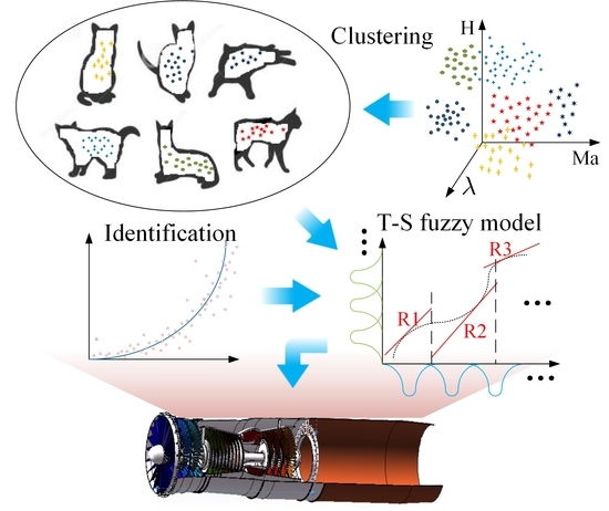
In this paper, in order to simulate engine strong nonlinear dynamics with high accuracy and fidelity and low complexity, we explored T–S fuzzy modeling for engines by using a clustering and identification approach. Via clustering of the engine dynamics, we formed a series of rough T–S fuzzy models for aircraft engine nonlinear dynamics in the flight envelope. For each rough T–S fuzzy model, the maximum–minimum distance-based fuzzy c-means (MMD-FCM) algorithm was proposed to determine the fuzzy rule numbers and consequent engine linear models. Input and output sequences of aircraft engines were employed to identify the premise parameters with the least square method (LSM).

This paper offers three main contributions. First, clustering with dominant poles of engine linear models in the entire flight envelope guarantees that similar dynamics of engines can be simulated by a T–S fuzzy model, and this T–S fuzzy model can have fewer fuzzy rules, which is beneficial to reducing model complexity. Second, the proposed MMD-FCM algorithm guarantees that the clustering process that determines the fuzzy rule numbers and consequent engine linear models in each T–S fuzzy model is stable and more reasonable. Third, the identification of steady and transient data improves the accuracy of the T–S fuzzy model during the engine dynamic process.

2. Main Philosophy of T–S Fuzzy Modeling for Aircraft Engines

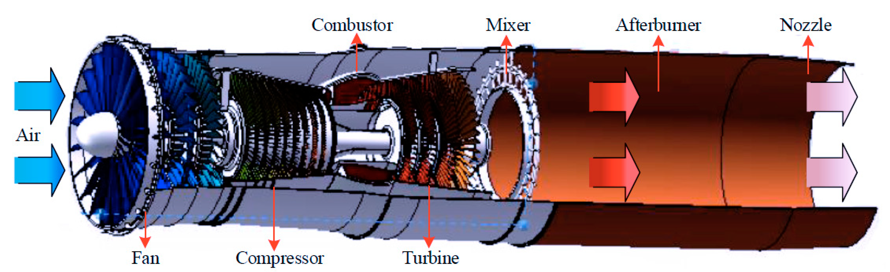
Aircraft engines are a complex aero-thermodynamic system. Figure 1 depicts the major structure of a turbofan engine, a kind of aircraft engine comprising an inlet, fan, compressor, combustor, high-pressure turbine, low-pressure turbine, afterburner and nozzle.

Consider a turbofan engine described as a series of T–S fuzzy models $F_k,k=1,2,\cdots ,N_k$ as

$$\begin{array}{ll}{F}_k:R^i:\mathrm{IF}\hspace{1em}& v_{k1} \mathrm{is} L_{k1}^i,v_{k1} \mathrm{is} L_{k1}^i,\cdots ,v_{k1} \mathrm{is} L_{k1}^i,\\ \hfill \mathrm{Then}& \\ & \dot{x}(t)=A_{ki}^{C}x(t)+B_{ki}^{C}u(t),\\ & y(t)=C_{ki}^{C}x(t)+D_{ki}^{C}u(t),\end{array}$$

(1)

where $i=1,2,\cdots ,N_k^c$ is the number of fuzzy rules, $v_{ki}$ is the premises without dependence on the system state, $L_{ki}^i,(l=1,2,\cdots g)$ is the antecedent fuzzy set, $t\in R$ is time, $x(t)\in R^n$ is the engine state, $u(t)\in R^m$ is the control input, $y(t)\in R^n$ is the engine output and $A_{ki}^C$, $B_{ki}^C$, $C_{ki}^C$ and $D_{ki}^C$ are the known real matrices with appropriate dimensions.

Hence, by using a weighted-average defuzzifier, the global T–S fuzzy model can be inferred as

$$\begin{array}{l}\dot{x}(t)=A_{zk}x(t)+B_{zk}u(t),\\ y(t)=C_{zk}x(t)+D_{zk}u(t),\end{array}$$

(2)

where

$$\begin{array}{l}{A}_{zk}={\displaystyle \sum _{i=1}^{r_k}{h}_{ki}\left(v_k(t)\right)A_{ki}^C,B_{zk}={\displaystyle \sum _{i=1}^{r_k}{h}_{ki}\left(v_k(t)\right)B_{ki}^C,}}\\ C_{zk}={\displaystyle \sum _{i=1}^{r_k}{h}_{ki}\left(v_k(t)\right)C_{ki}^C,D_{zk}={\displaystyle \sum _{i=1}^{r_k}{h}_{ki}}\left(v_k(t)\right)D_{ki}^C,}\\ v_k=[v_{k1},v_{k2},\cdots ,v_{kg}{]}^T,\end{array}$$

(3)

with $h_{ki}(v(t))={\mu }_{ki}(v_k(t))/{\displaystyle \sum _{i=1}^{r_k}{\mu }_{ki}(v_k(t))}$, ${\displaystyle \sum _{i=1}^{r_k}{h}_{ki}(v_k(t))}=1$ and $h_{ki}(v_k(t))>0$. Here, ${\mu }_{ki}(v_k(t))={\displaystyle \prod _{j=1}^g{L}_{kij}(v_{kj}(t))}$ and $L_{kij}(v_{kj}(t))$ is the degree of membership function of $v_{kj}$ in the fuzzy sets $L_{kj}^i$, while $L_{kij}(v_{kj}(t))=\exp \left(-\frac{{(v_{kj}-{\gamma }_{ki})}^2}{{\sigma }_{ij}}\right)$ is a Gaussian function.

Remark 1.

Since the dynamic characteristics of aircraft engines vary significantly and nonlinearly under different inlet conditions and different operation conditions, a single T–S fuzzy model has difficulty precisely describing the engine behaviors in the full flight envelope. In this paper, we intend to adopt multiple T–S fuzzy models$F_k$to simulate more comprehensive engine dynamics in the full flight envelope.

Based on this modeling philosophy, we propose the following approach to the engine T–S fuzzy modeling:

Step 1. Under an operating condition, linearize an aircraft engine to a state space and adopt the dominant eigenvalue of the system matrix to demonstrate the engine dynamics.

Step 2. For a given number of the engine T–S fuzzy model $N_k$, cluster the engine dynamics to determine the sub-region of the flight envelop in which the T–S fuzzy model $F_k$ works.

Step 3. In each sub-region, use the mixed-F statistic method to determine the number of fuzzy rules $N_k^C$ required to guarantee the engine dynamics in each rule are distinguished.

Step 4. In each sub-region, use an improved fuzzy C-means (FCM) to determine the consequence (the engine state-space model) in the $i\mathrm{th}$ rule.

Step 5. Using the data from the engine static and dynamic process and the least square method, modify the engine’s T–S fuzzy model.

In Section 3, we will present the details of the above modeling steps.

3. Engine T–S Fuzzy Modeling

3.1. Engine Dynamic Clustering Based on K-Means Algorithm

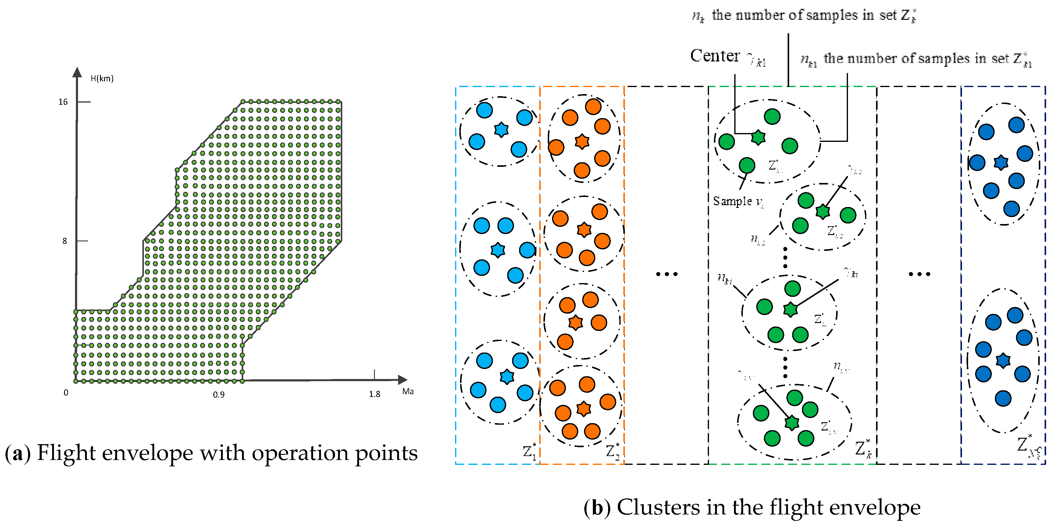
Under an operation point in the flight envelope (shown in Figure 2a), an aircraft engine is described as

$$\begin{array}{l}\dot{x}(t)=A_{i}x(t)+B_{i}u(t),\\ \mathrm{y}(t)=C_{i}x(t)+D_{i}u(t),\end{array}$$

(4)

where $i=1,2,\cdots ,N_s$, $A_i$, $B_i$, $C_i$ and $D_i$ are constant matrices with appropriate dimensions. The eigenvalue of $A_i$ is ${\zeta }_{ij}(A_i)$, $j=1,2\cdots ,n$. For all ${\zeta }_{ij}(A_i)$, we define the dominant pole

$${\zeta }_i(A_i)=\left\{{\zeta }_{ij}(A_i)|\min \left(\left|\mathrm{Re}({\zeta }_{ij})\right|\right)\right\} ,$$

(5)

where $\mathrm{Re}(·)$ is the real part of a complex number. Therefore, the sample set of engine dynamics is $Z=({\zeta }_1,{\zeta }_2,\cdots ,{\zeta }_{N_s})$. Suppose that all samples in the set $Z$ are clustered into $(Z_1,Z_2,\cdots Z_{N_k})$ and the sample number in the cluster $Z_k$ is ${\overline{n}}_k$.

Define the value function as

$$J_{DY}={\displaystyle \sum _{k=1}^{N_k}{\displaystyle \sum _{{\zeta }_i\in Z}\Vert {\zeta }_i-{\xi }^{\ast }{}_k{\Vert }_2^2}} ,$$

(6)

where ${\xi }_k^{\ast }=\frac{1}{{\overline{n}}_k}{\displaystyle \sum _{{\zeta }_i\in Z_k}{\zeta }_i}$ is the cluster center of all samples in cluster $Z_k$. By a K-means clustering algorithm [25], we obtain $N_k$ which minimizes the value function $J_{DY}$ and the corresponding clustering sets $(Z_1^{\ast },Z_2^{\ast },\cdots ,Z_{N_k}^{\ast })$.

Remark 2.

By clustering ${\zeta }_i$, we actually gather the similar dynamics of an engine together in the flight envelope. If the matrix $A_i$ depends on the flight height and Mach number of an engine operation, this clustering means we divide the flight envelope (Figure 2a) into $N_k$ sub-regions $(Z_1^{\ast },Z_2^{\ast },\cdots ,Z_{N_k}^{\ast })$. For each sub-region, the T–S fuzzy model $F_k$ in Equation (1) is established to simulate the engine behavior. To show the details of clustering clearer, we neglect the real shape of these sub-regions and demonstrate them with rectangles as shown in Figure 2b. Moreover, Figure 2b also illustrates the clustering details in the sub-regions in Section 3.2.

3.2. Determination of Fuzzy Rule Number $N_k^c$ Based on Mixed-F Statistics

Next, we use the mixed-F statistics-based FCM algorithm to determine an optimal fuzzy rule number $N_k^{c\ast }$, $k=1,2,\cdots N_k$ in Equation (1). Therefore, $N_k^{c\ast }$ is also the number of clustering class.

Define the value function as

$$J_{FL,k}({\mathsf{\Omega }}_k,v_k)={\displaystyle \sum _{i=1}^{N_k^C}{\displaystyle \sum _{j=1}^{n_k}{\omega }_{kij}^K{d}_{kij}^2}} ,$$

(7)

where ${\mathsf{\Omega }}_k=[{\omega }_{kij}]\in R^{N_k^c\times N_s}$ is the weight matrix and ${\omega }_{kij}$ is the membership degree of a sample that belongs to the class $i$ and satisfies

$${\displaystyle \sum _{i=1}^{N_k^C}{\omega }_{kij}=1},j=1,2,\cdots ,n_k.$$

(8)

$N_k^c$ is the number of clustering center in sub-region $Z_k^{\ast }$, $n_k$ is the sample number in the sub-set $Z_k^{\ast }$ and $K\in [1,\infty )$ is fuzzy weight index:

$$d_{kij}={\Vert v_{ki}-{\gamma }_{kj}\Vert }_2.$$

(9)

Here, the Euclidean distance $d_{kij}$ is the distance between the sample $v_{ki}$ and the clustering center ${\gamma }_{kj}$ in the sub-set $Z_k^{\ast }$. It is worth noting that Equation (8) suggests the sub-set $Z_k^{\ast }$ is further clustered into $N_k^c$ classes $Z_{k1}^{\ast },Z_{k2}^{\ast },\cdots ,Z_{k{N}_k^c}^{\ast }$.

In the sub-region $Z_k^{\ast }$, suppose the clustering centers are $O_{k1},O_{k2},\cdots ,O_{k,N_k^c}$. According to Equations (7) and (8), we form a Lagrange equation:

$${\overline{J}}_k({\mathsf{\Omega }}_k,v_k,{\lambda }_{k1},\cdots ,{\lambda }_{k{N}_k^c})={\displaystyle \sum _{i=1}^{N_k^C}{\displaystyle \sum _{j=1}^{N_s}{\omega }_{kij}^k}}{\Vert v_{ki}-{\gamma }_j\Vert }_2^2+{\displaystyle \sum _{j=1}^{N_s}{\lambda }_{kj}}\left({\displaystyle \sum _{i=1}^{N_k^C}{\omega }_{kij}-1}\right) ,$$

(10)

where ${\lambda }_{kj}$ is the Lagrange multiplier. Set the gradient of ${\overline{J}}_k$ to 0, namely,

$$\frac{\partial {\overline{J}}_k}{\partial {\omega }_{kij}}=\kappa {\omega }_{kij}^{\kappa -1}{d}_{kij}^2-{\lambda }_{kj}=0 ,$$

(11)

$$\frac{\partial {\overline{J}}_k}{\partial {\lambda }_{kj}}={\displaystyle \sum _{i=1}^{N_k^C}{\omega }_{kij}-1}=0 ,$$

(12)

$$\frac{\partial {\overline{J}}_k}{\partial {\gamma }_{kj}}=-2{\displaystyle \sum _{j=1}^{N_s}{\omega }_{kij}^{\kappa }}\left(v_{ki}-{\gamma }_{kj}\right)=0 ,$$

(13)

giving us

$${\omega }_{kij}={\left(\frac{{\lambda }_{kj}}{\kappa d_{kij}^2}\right)}^{\frac{1}{\kappa -1}}.$$

(14)

$${\left(\frac{{\lambda }_{kj}}{\kappa }\right)}^{\frac{1}{\kappa -1}}={{\displaystyle \sum _{i=1}^{N_k^C}\left(\frac{1}{d_{kij}^2}\right)}}^{-\frac{1}{\kappa -1}} .$$

(15)

Introduce Equations (15) into (14), giving us

$${\omega }_{kij}={\left(\frac{1}{d_{kij}^2}\right)}^{\frac{1}{\kappa -1}}{{\displaystyle \sum _{i=1}^{N_k^C}\left(d_{kij}^2\right)}}^{\frac{1}{\kappa -1}}.$$

(16)

Using Equations (13) and (16), this yields

$${\gamma }_{kj}=\frac{{\displaystyle \sum _{j=1}^{N_s}{\omega }_{kij}^{\kappa }{v}_{ki}}}{{\displaystyle \sum _{j=1}^{N_s}{\omega }_{kij}^{\kappa }}}.$$

(17)

Further, for the clustering number $N_k^c$ in the sub-region $Z_k^{\ast }$, we define the mixed-F statistic as

$$F_{k,mix}=\frac{g}{{\displaystyle \sum _{i=1}^g\frac{1}{F_k(l)}}} ,$$

(18)

with

$$F_k(l)=\frac{{\displaystyle \sum _{i=1}^{N_k^C}{n}_{ki}{({\gamma }_{ki,l}-{\overline{\gamma }}_{k,l})}^2(n_k-N_k^c)}}{{\displaystyle \sum _{i=1}^{N_k^C}{\displaystyle \sum _{j=1}^{n_{ki}}{(v_{kij,l}-{\gamma }_{ki,l})}^2(N_k^c-1)}}}.$$

(19)

Here $n_{ki}$ is the sample number in the sub-set $Z_{ki}^{\ast }$, and ${\gamma }_{ki,j}$ is the $lth$ entry of ${\gamma }_{ki}$ and

$${\overline{\gamma }}_{k,l}=\frac{1}{N_k^c}{\displaystyle \sum _{i=1}^{N_k^C}{\gamma }_{ki,l}}.$$

(20)

Let $N_k^C=1,2,\cdots ,r_k$, and using Equations (16)–(18) we can calculate a series of $F_{k,mix}$, namely, $F_{k1,mix},F_{k2,mix},\cdots ,F_{k{N}_k^C,mix}$.

Define

$$N_k^{C\ast }:\left\{i|\max (F_{ki,mix},i=1,2\cdots ,r_k)\right\} ,$$

(21)

and we obtain the optimal fuzzy rule number $N_k^{C\ast }$ in regard of the mixed-F statistic $F_{k,mix}$.

Remark 3.

In the FCM algorithm, the clustering number $N_k^C$ directly affects the performance of the T–S fuzzy model. Too many rules might lead to model redundancy, and fewer rules could cause poor accuracy in approximating the physical system with the fuzzy model. We adopt the mixed-F statistic as an index to seek an optimal $N_k^C$. The numerator of the mixed-F statistic means the distance between classes, and the denominator means the distance between data points and clustering center. Therefore, the maximum of the mixed-F statistic implies the farthest distance between every pair of classes and the optimal classification.

3.3. Consequence Modeling Based on the MMD-FCM Algorithm

Using Equation (21), we determine an optimal fuzzy rule number for each fuzzy model $F_k$. In this subsection, we propose the MMD-FCM algorithm for modeling the consequences of each fuzzy rule in $F_k$.

In the sub-region $Z_k^{\ast }$, let the arbitrary vector $v_{ki}$, $i=1,2,\cdots ,n_k$, as the initial of the first center $z_{k1}$, namely, $z_{k1}=v_{ki}$.

Using

$$z_{k2}=\left(v_{kj}|\underset{\mathrm{j}}{\max }\left({\Vert v_{kj}-z_{k1}\Vert }_2,j=1,2,\cdots ,n_k,j\ne i\right)\right),$$

(22)

we determine the initial of the second center $z_{k2}$. Let

$$D_{kij,l}={\Vert v_{kj}-z_{ki}\Vert }_2,$$

(23)

and the $(l+1)\mathrm{th}$ center $z_{k,l+1}$ is

$$z_{l+1}=\left(v_{kj}|\underset{j}{\max }\left(\min \left\{D_{kij,l}\right\}\right)\right),i=1,2,\cdots ,l,j=1,2\cdots ,n_k.$$

(24)

Using Equations (23)–(24), we can get all the initial centers $Z_k=\left(z_{k1},z_{k2},\cdots ,z_{k{N}_k^C}\right)$ in $F_k$.

We regard $Z_k=\left(z_{k1},z_{k2},\cdots ,z_{k{N}_k^C}\right)$ as the initial centers and introduce it into Equation (16). Give $N_k^{C\ast }$ by Equation (21) and choose the appropriate threshold value $\epsilon$, and we can calculate membership matrix $\mathsf{\Omega }$;

Next we can calculate the value function $J_{FL}(\mathsf{\Omega },v)$ using Equation (7). If $J_{FL}(\mathsf{\Omega },v)<\epsilon$, the algorithm stops; if not, continue to calculate ${\gamma }_{kj}$ using Equation (17). Repeat this process until satisfying $J_{FL}(\mathsf{\Omega },v)<\epsilon$.

Through the above process, optimal center ${\gamma }_{ki}^{\ast },i=1,2,\cdots ,N_k^C$ in $F_k$ can be obtained. In ${\gamma }_{ki}^{\ast }$, we linearize the nonlinear model of an aeroengine using the fitting method to get the corresponding linear model $A_{ki}^C$, $B_{ki}^C$, $C_{ki}^C$ and $D_{ki}^C$.

Remark 4.

The FCM algorithm uses the gradient method to search for optimal clustering [26]. The initials affect the searching gradient, and inappropriate initials will lead to unstable clustering results or local minimums. In this paper, we adopt the maximum and minimum distance (MMD) to obtain the appropriate initials for FCM [27]. The MMD collaborates with FCM, namely the MMD-FCM, to achieve a stable clustering result.

3.4. Model Parameter Identification with LSM

In order to make the T–S fuzzy model closer to the actual system, after determining the fuzzy consequent parts $A_{ki}^C$, $B_{ki}^C$, $C_{ki}^C$ and $D_{ki}^C$, the parameter ${\sigma }_{ij}$ in a Gaussian function $L_{kij}\left(v_{kj}(t)\right)=\exp \left(-\frac{{(v_{kj}-{\gamma }_{ki})}^2}{{\sigma }_{ij}}\right)$ will be identified as a smooth parameter, and the selection of parameter will affect the smoothness of the system. A smaller ${\sigma }_{ij}$ may lead to a small fitting error, but it is difficult to generalize the data of non-training points. A larger ${\sigma }_{ij}$ may lead to a good generalization performance, but it could cause larger errors in the training data. Therefore, the appropriate parameter ${\sigma }_{ij}$ should be selected to maintain the balance between fitting and generalization. In this paper, the least square method is adopted to identify smooth parameters. Given the input sequence $△u$, we can achieve output sequence $△y$ and define the value function $J_{Ls}={{\displaystyle \sum \Vert △y-△\overline{y}\Vert }}_2^2$, where $△\overline{y}$ is the output of fuzzy model with the input sequence $△u$. To minimize $J_{Ls}$ we should achieve a reasonable parameter ${\sigma }_{ij}$. In order to avoid too large or too small of a parameter ${\sigma }_{ij}$ to affect the fitting and generalization performance of the fuzzy system, the upper and lower bounds of identification are set.

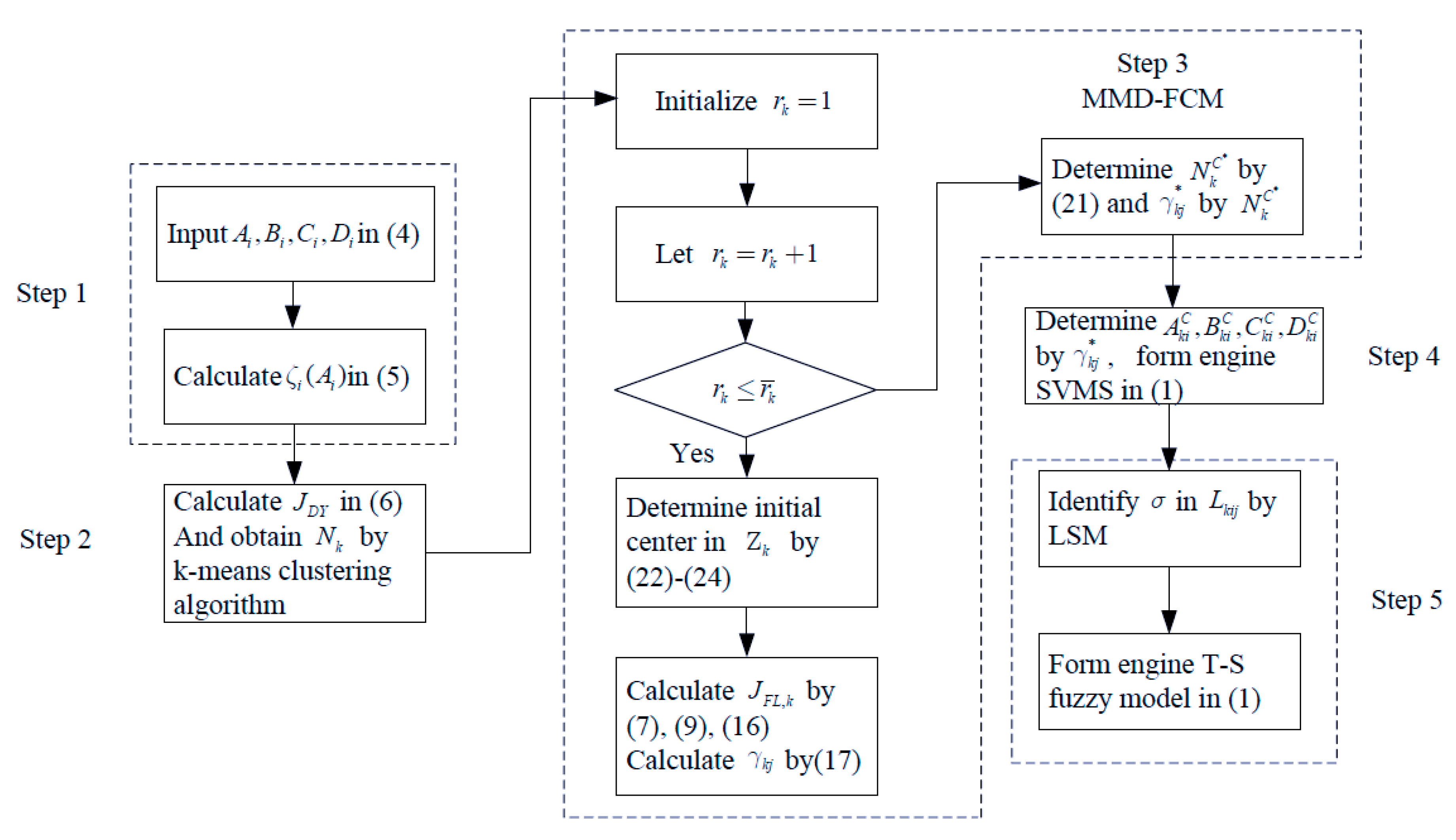
3.5. T–S Fuzzy Modeling Process

We summarize the engine’s T–S fuzzy modeling process in Figure 3. As mentioned in Section 2, the process of T–S fuzzy modeling for an engine involves five steps. In Figure 3, we match the corresponding process blocks with the five steps. It is shown that the MMD-FCM is the core algorithm in the modeling. It is noted that, in this process, ${\overline{r}}_k$ is the upper bound of $r_k$. Let $r_k=1,2,\cdots ,{\overline{r}}_k$ and obtain the optimal $N_k^{C\ast }$ in (1,2 $\cdots$, ${\overline{r}}_k$) by MMD-FCM. Therefore, when $r_k>{\overline{r}}_k$, the search of $N_k^{C\ast }$ is ended and the transition occurs.

4. An Illustrative Example

4.1. The T–S Fuzzy Modeling for a Turbofan Engine

Consider a turbofan engine as shown in Figure 1 and described as the T–S fuzzy model (Equation (1)).

We established a grid of a flight envelope depicting every 0.5 km and 0.05 Mach number. Hence, the 725 grid vertices were yields in the flight envelope. Each vertex demonstrated the turbofan state-space model shown in Equation (4). Therefore, N_s = 725. The 725 dominant poles of matrices A_i (i = 1,2,…, 725) of all state-space models were calculated. Due to the space limitation, we prefer not to present these calculation results. Next, let N_k = 4. By the K-means algorithm and dominant poles, the operation points in the flight envelope were clustered into four classes, which means the flight envelope are divided into four sub-regions based on the engine dynamics (Figure 4a). Therefore, $n_1=234$, $n_2=172$, $n_3=240$ and $n_4=79$. Let κ = 1.5 and r_k = 1,2,…, 20. Using Equations (16)–(20), we calculate the mixed-F statistics for regions 1–4 and depict the calculations in Figure 4b.

Figure 4 shows different T–S fuzzy models built in different sub-regions, with different mixed-F statistics calculated under different classification numbers. When the mixed-F statistics reached the maximum value, the corresponding clustering number is the best. Hence, for regions 1–4, the best classification numbers were 6, 10, 9 and 6, namely, $N_1^{C\ast }=6$, $N_2^{C\ast }=10$, $N_3^{C\ast }=9$ and $N_4^{C\ast }=6$.

Using Equations (23)–(24), we can get all the initial centers ${\mathrm{Z}}_k=\left(z_{k1},z_{k2},\cdots ,z_{k{N}_k^c}\right)$, $k=1,2,3,4$, $N_k^{C\ast }=6,10,9,6$. Using Equations (7) and (17), we obtain the optimal centers of regions 1–4. The positions of the optimal centers are shown in Figure 5 and their coordinates in the flight envelope are listed in

Table 1. Cluster centers of the flight envelope.

	Center1	Center2	Center3	Center4	Center5	Center6	Center7	Center8	Center9	Center10
R1	(0.7,10.9)	(1.4,15.2)	(1.1,15.1)	(0.8,9.7)	(1.1,11.6)	(1.2,13.3)	(1.2,13.3)	(0.6,8.0)	(0.4,6.8)	*
R2	(0.9,7.2)	(1.5,12.5)	(0.1,2.7)	(0.7,5.9)	(0.4,3.7)	(1.2,9.8)	*	*	*	*
R3	(0.5,0.9)	(1.5,10.4)	(1.2,7.2)	(0.9,4.7)	(0.07,0.4)	(1.1,0.6)	(0.8,3.3)	(1.3,8.9)	(0.3,0.6)	(0.6,2.1)
R4	(0.9,1.3)	(1.5,8.4)	(1.2,6.0)	(0.7,0.3)	(1.1,4.1)	(1.3,6.7)	*	*	*	*

*: No center point.

.

The clustering center results are shown in Table 1 below.

The selected initial values were ${\sigma }_{ki}(\cdot )=0.3$. The transition states at 1, 1.2 and 1.4 s for 725 points selected in the envelope of the nonlinear system under a 3% fuel step input at the conversion speed of the high-pressure rotor were added to train with the output data of the steady-state response. The smooth parameter of the Mach number membership ${\sigma }_{ki}(Ma)$ is listed in

Table 2. Mach number membership ${\sigma }_{ki}(Ma)$.

	${\mathit{\sigma }}_{\mathit{k}1}$	${\mathit{\sigma }}_{\mathit{k}2}$	${\mathit{\sigma }}_{\mathit{k}3}$	${\mathit{\sigma }}_{\mathit{k}4}$	${\mathit{\sigma }}_{\mathit{k}5}$	${\mathit{\sigma }}_{\mathit{k}6}$	${\mathit{\sigma }}_{\mathit{k}7}$	${\mathit{\sigma }}_{\mathit{k}8}$	${\mathit{\sigma }}_{\mathit{k}9}$	${\mathit{\sigma }}_{\mathit{k}10}$
R1	0.4271	0.2007	0.2001	0.2490	0.2007	0.3512	0.3001	0.3102	0.3008	*
R2	0.2001	1.7398	0.4001	0.6681	0.2025	0.3318	*	*	*	*
R3	0.2081	0.9362	0.2156	0.2187	0.4251	0.4488	0.3479	0.26645	0.5151	0.2051
R4	0.2901	0.9895	0.2412	0.3346	0.2503	0.2227	*	*	*	*

*: No value.

, and the smooth parameter of height membership ${\sigma }_{ki}(H)$ is listed in

Table 3. Mach number membership ${\sigma }_{ki}(H)$.

	${\mathit{\sigma }}_{\mathit{k}1}$	${\mathit{\sigma }}_{\mathit{k}2}$	${\mathit{\sigma }}_{\mathit{k}3}$	${\mathit{\sigma }}_{\mathit{k}4}$	${\mathit{\sigma }}_{\mathit{k}5}$	${\mathit{\sigma }}_{\mathit{k}6}$	${\mathit{\sigma }}_{\mathit{k}7}$	${\mathit{\sigma }}_{\mathit{k}8}$	${\mathit{\sigma }}_{\mathit{k}9}$	${\mathit{\sigma }}_{\mathit{k}10}$
R1	0.2048	0.3650	0.2949	0.2005	0.2006	0.2049	0.2053	0.4228	0.2981	*
R2	0.2005	0.2001	0.2008	0.2008	0.2006	1.7143	*	*	*	*
R3	0.2095	0.4076	0.2013	0.2057	1.2483	0.9086	1.4999	0.5464	0.2000	0.2079
R4	0.3158	0.2789	0.2874	0.2786	0.2809	0.2905	*	*	*	*

*: No value.

.

4.2. Model Verification

In order to verify the feasibility of the proposed T–S fuzzy modeling method in the full envelope, simulation verification was carried out under different flight conditions. Because the turbofan component-level nonlinear models can simulate real turbofan engines with high accuracy and fidelity [1,28], in the simulation, a turbofan nonlinear model was adopted as the baseline. The responses of the turbofan T–S fuzzy model were compared to those of the nonlinear model in order to verify the T–S fuzzy model.

Under a 3% fuel step input, the responses of the T–S fuzzy model with and without LSM identification (LSM-ID) were compared with those of the nonlinear model shown in Figure 6 and Figure 7. The relative error for the steady error and the RMSE for all errors are shown in Figure 8 and Figure 9.

Figure 6 and Figure 7 show that, according to the LSM-ID, the relative steady-state error of T–S fuzzy models after identification between nonlinear models was less than 5%. Compared to the T–S fuzzy models without LSM-ID, the T–S fuzzy models with LSM-ID had less relative errors.

In Figure 8b and Figure 9b it can be seen that the dynamic errors of T₄₃ and EPR were bigger than those of N_L and N_H. The possible reason is that T₄₃ and EPR were formulated as a linear function of N_L and N_H in Equation (1). In fact, the relationships between them are a nonlinear. These modeling errors may cause the dynamic errors of $T_{43}$ and EPR.

Moreover, in order to verify the generalization of the resulted model within the flight envelope, non-identification operation points in the flight envelope were selected for simulation. The simulation conditions were the same as those in Figure 6 and Figure 8. The engine responses are shown in Figure 10 and Figure 11 and the relative error and RMSE of the T–S fuzzy models with/without LSM-ID are depicted in Figure 12 and Figure 13. Figure 12 and Figure 13 show that, at non-identification operation points, the outputs of the fuzzy model with/without LSM-ID were close to those of the nonlinear model. Figure 12 and Figure 13 show that the relative errors of the T–S fuzzy model with LSM-ID at non-identification operation points were slightly bigger than those at the identification points, which indicates that the fuzzy model had good generalization ability.

5. Conclusions

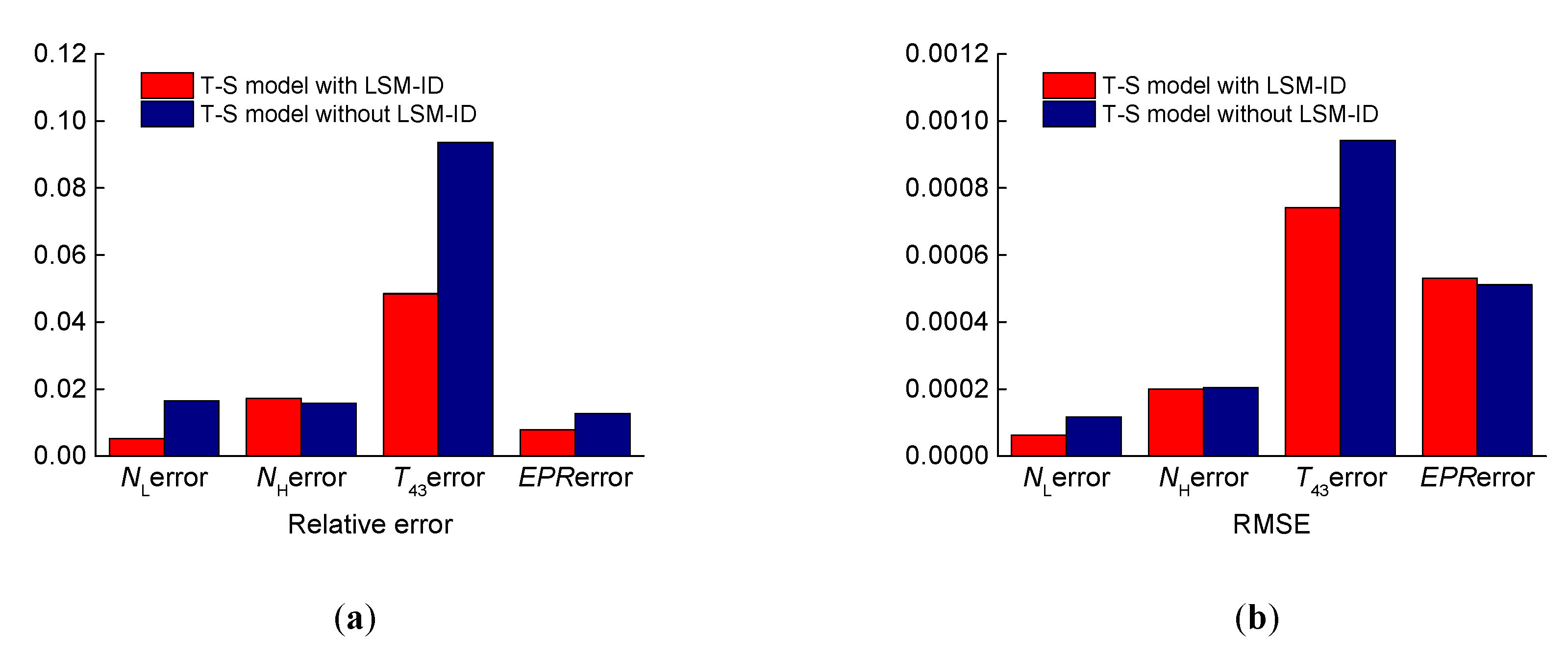
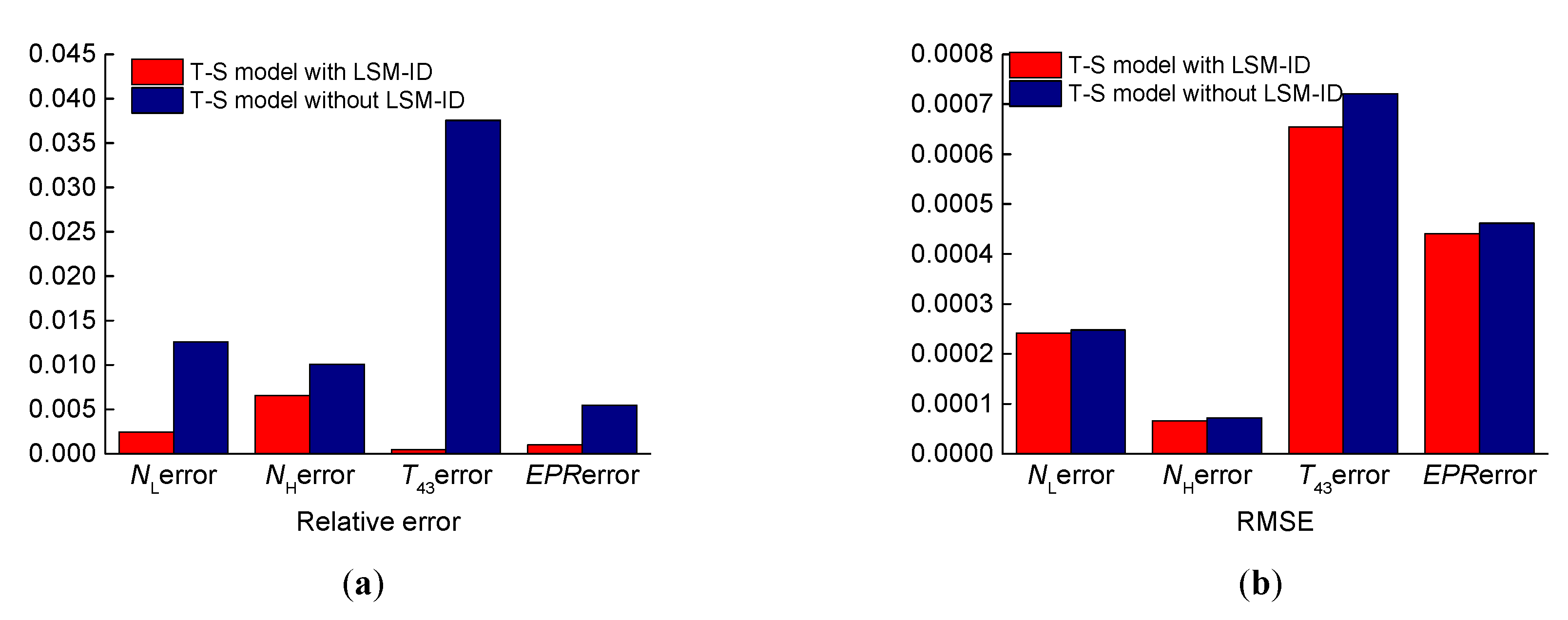
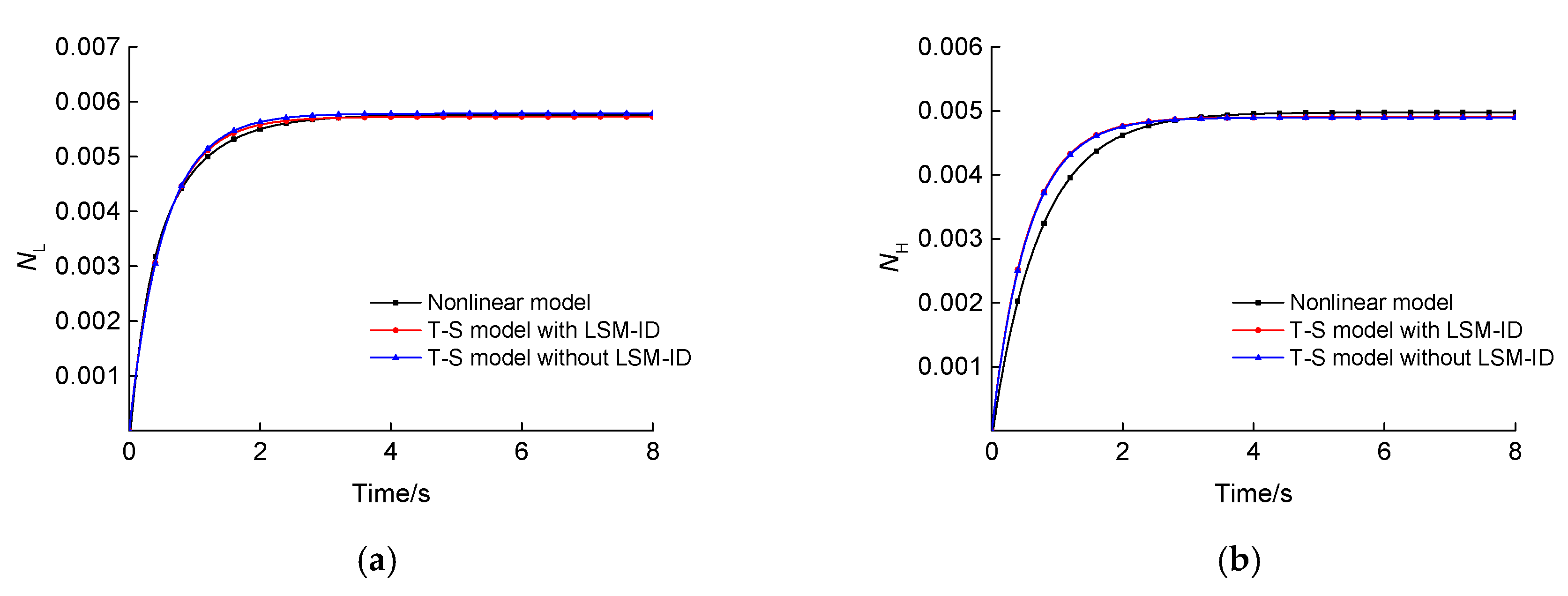
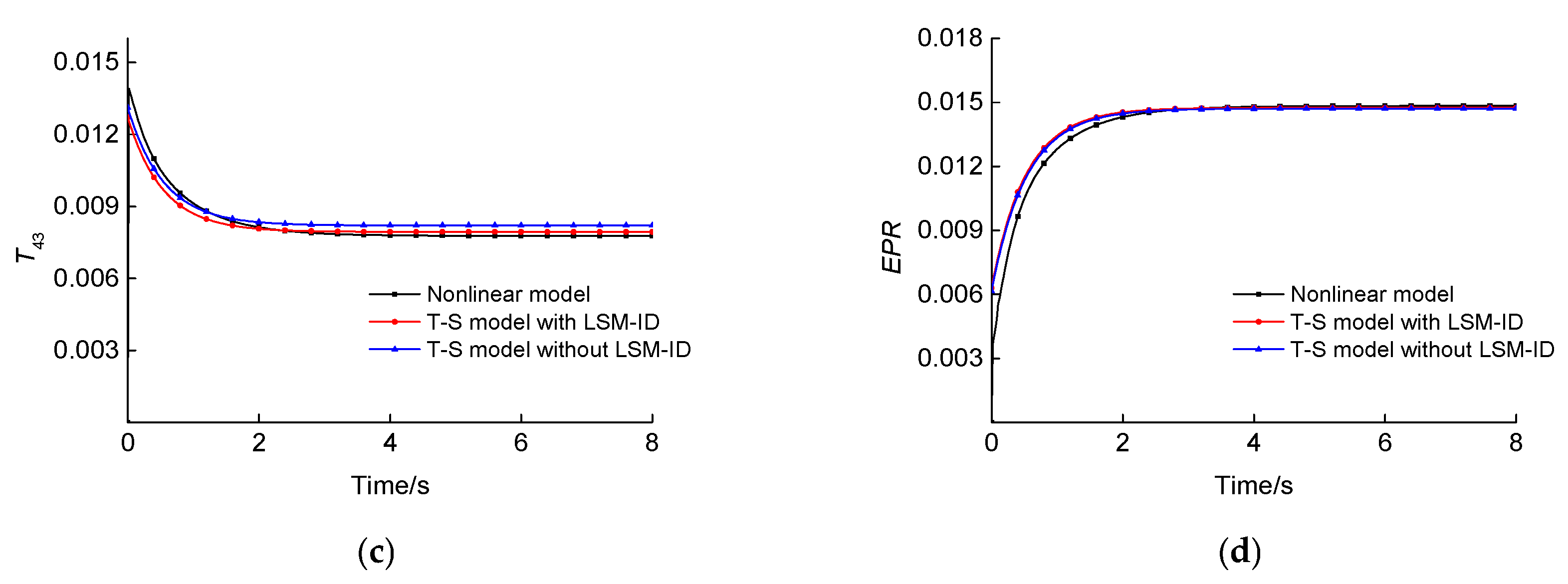
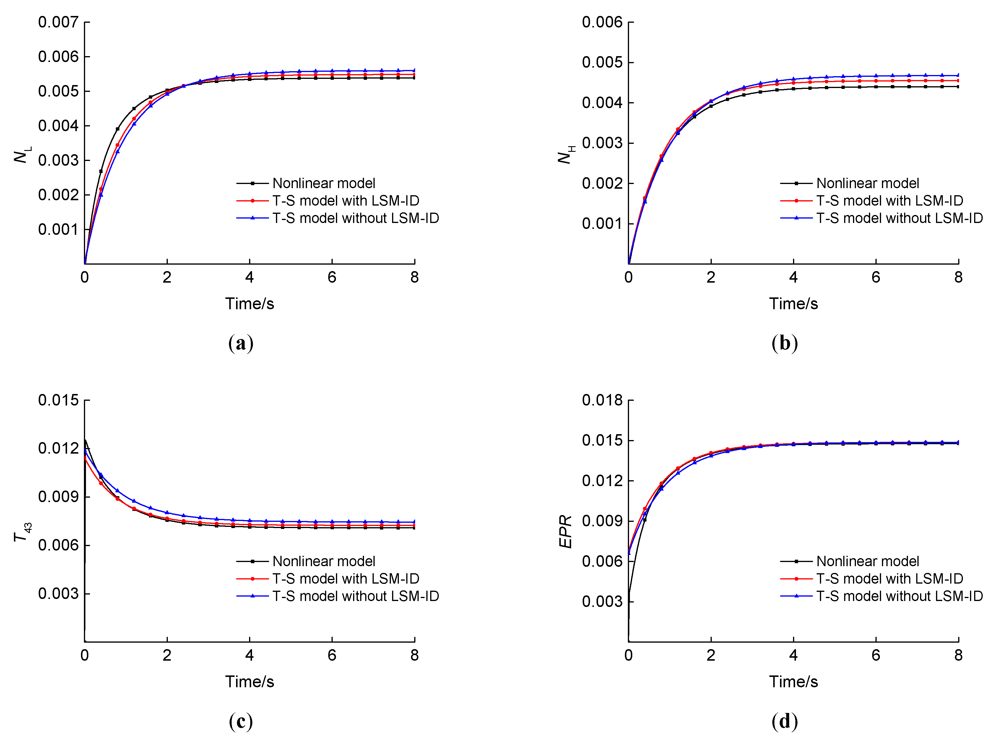
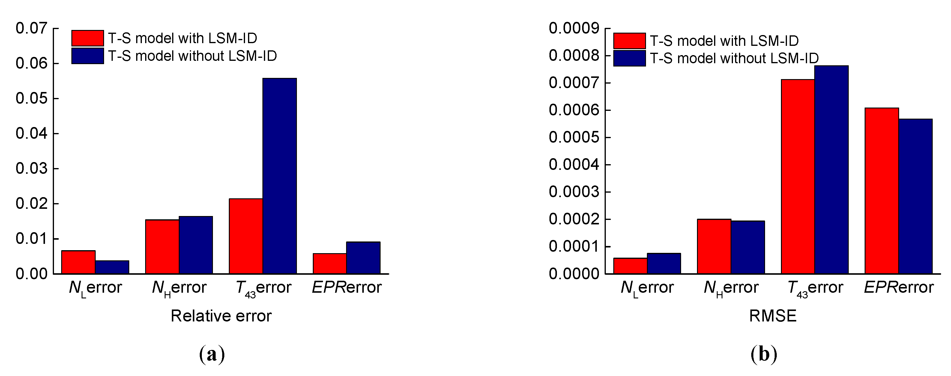
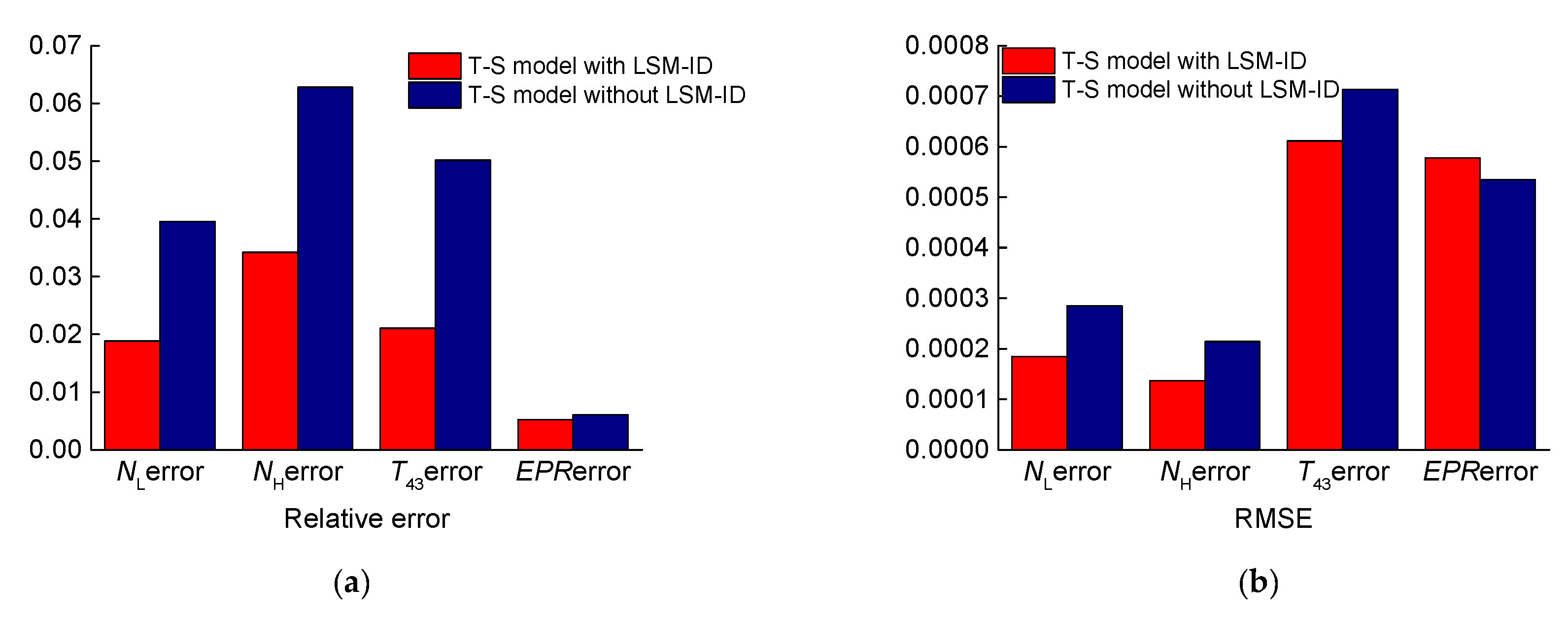
In this paper, an improved FCM algorithm was used to achieve the fuzzy division of a flight envelope, and the fuzzy division regions and clustering centers were obtained. The state-space model was used as the subsequent part of the T–S fuzzy model, and the weight of the T–S fuzzy model was identified, allowing the T–S fuzzy model of an aeroengine within the full envelope to be obtained. (1) By comparing with the nonlinear model, it was proven that this modeling method has good accuracy, and all the four steady-state outputs met an error of <5%. (2) The identification method proposed in this paper had high identification accuracy and strong generalization, so this identification algorithm can also be used for the identification of other complex nonlinear systems with time-varying uncertainties.

Via the positive results of the model verification, further efforts are encouraged. (1) The engine data in bench test data and flight data could be used for further model verification, which would facilitate the application of the resulting T–S fuzzy model to real turbofan engines. (2) The proposed modeling algorithm could be applied to nonlinear system with large-scale nonlinear dynamics, such as turboshaft engines, electric pumps and mechanical hydraulic systems.

References

1. Pan, M.; Chen, Q.; Zhou, Y.; Zhou, W.; Huang, J. An approach with multi-dynamics for turbofan engine modeling. Acta Aeronaut. Astronaut. Sin. 2019, 40, 94–105. (In Chinese) [Google Scholar]
2. Zadeh, L.A. Fuzzy Sets. Inf. Control. 1965, 8, 338–353. [Google Scholar] [CrossRef]
3. Zhang, H.; He, X. Fuzzy Adaptive Control and Its Application, 1st ed.; Beihang University Press: Beijing, China, 2002; pp. 10–35. ISBN 7-81077-119-1. [Google Scholar]
4. Grzegorzewski, P. On Separability of Fuzzy Relations. Int. J. Fuzzy Log. Intell. Syst. 2017, 17, 137–144. [Google Scholar] [CrossRef] [Green Version]
5. Takagi, T.; Sugeno, M. Fuzzy Identification of Systems and Its Applications to Modeling and Control. IEEE Trans. Syst. Man. Cybern. 1985, 15, 116–132. [Google Scholar] [CrossRef]
6. Sugeno, M.; Yasukawa, T. Linguistic modeling based on numerical data. In Proceedings of the International Fuzzy Systems Association World Congress, Brussels, Belgium, 7–12 July 1991; pp. 264–267. [Google Scholar]
7. Tanaka, K.; Wang, H. Fuzzy Control. Systems Design and Analysis: A Linear Matrix Inequality Approach, 3rd ed.; John Wiley & Sons: Hoboken, NJ, USA, 2002; pp. 2011–2013. ISBN 0-471-33459-6. [Google Scholar]
8. Abonyi, J.; Babuska, R.; Szeifert, F. Modified Gath-Geva fuzzy clustering for identification of Takagi-Sugeno fuzzy models. IEEE Trans. Syst. Man. Cybern. B Cybern. 2002, 32, 612–621. [Google Scholar] [CrossRef] [PubMed]
9. Hoppner, F.; Klawonn, F. Improved fuzzy partitions for fuzzy regression models. Int. J. Approx. Reason. 2003, 32, 85–102. [Google Scholar] [CrossRef] [Green Version]
10. Li, M.; Liu, Z.; Nian, X.; Tan, W. Method of nonlinear systems identification with fuzzy clustering based on Takagi-Sugeno model. Comput. Eng. Appl. 2007, 43, 139–241. (In Chinese) [Google Scholar]
11. Pal, K.; Mudi, R.; Pal, N.R. A new scheme for fuzzy rule-based system identification and its application to self-tuning fuzzy controllers. IEEE Trans. Syst. Man. Cybern. B Cybern. 2002, 32, 470–482. [Google Scholar] [CrossRef] [PubMed]
12. Gao, S.; Dou, X.; Gao, X. The temperature system identification of the PVC stripper tower top based on PSO-FCM optimized T-S model. In Proceedings of the 24th Chinese Control and Decision Conference, Taiyuan, ShanXi, China, 23–25 May 2012; pp. 2529–2532. [Google Scholar]
13. Zhao, M.; Wang, P.; Liang, J. Modeling of reference value of boiler operating parameters based on weighted fuzzy C-means clustering algorithm. Therm. Power Gener. 2019, 48, 12–17. (In Chinese) [Google Scholar]
14. Li, C.; Zhou, J.; Li, Q.; An, X.; Xiang, X. A new T–S fuzzy-modeling approach to identify a boiler—turbine system. Expert Syst. Appl. 2010, 37, 2214–2221. [Google Scholar] [CrossRef]
15. Moêz, S.; Chaari, A.; Fayçal, B. Takagi-Sugeno fuzzy model parameters identification based on fuzzy c-regression model clustering algorithm and particle swarm optimization. In Proceedings of the 16th IEEE Mediterranean Electrotechnical Conference, Yasmine Hammamet, Tunisia, 25–28 March 2012; pp. 1059–1062. [Google Scholar]
16. Mohamed, B.; Ahmed, T.; Lassad, H. New Allied Fuzzy C-Means algorithm for Takagi-Sugeno fuzzy model identification. In Proceedings of the International Conference on Electrical Engineering & Software Applications, Hammamet, Tunisia, 21–23 March 2013; pp. 1–7. [Google Scholar]
17. Yu, J.; Cheng, Q. The search range of optimal clustering number in fuzzy clustering method. Sci. China 2002, 32, 274–280. (In Chinese) [Google Scholar]
18. Bezdek, J.C.; Pal, N.R. Some new indexes of cluster validity. IEEE Trans. Syst. Man. Cybern. B Cybern. 2002, 28, 301–315. [Google Scholar] [CrossRef] [PubMed]
19. Xie, X.; Beni, G. A validity method for fuzzy clustering. IEEE Trans. Pattern Anal. Mach. Intell. 1991, 13, 841–847. [Google Scholar] [CrossRef]
20. Rezaee, M.R.; Lelieveldt, B.P.F.; Reiber, J.H.C. A new cluster validity index for the fuzzy c-mean. Pattern Recogn. Lett. 1998, 19, 237–246. [Google Scholar] [CrossRef]
21. Sun, C.; Wang, J.; Pan, J. Research on the Method of Determining the Optimal Class Number of Fuzzy Cluster. Fuzzy Syst. Math. 2001, 15, 89–92. (In Chinese) [Google Scholar]
22. Wang, C. Fault Diagnosis and Fault-Tolerant Control for Aeroengine with Sensor Fault Based on T-S Fuzzy Model. Master’s Thesis, Northeastern University, ShenYang, China, June 2013. (In Chinese). [Google Scholar]
23. Zhai, X.; Xie, S.; Miao, Z.; Peng, J.; Zhang, Z.; Wang, L. Fault detection of aero-engine non-linear distributed control system based on T-S fuzzy model. J. Aerosp. Power 2013, 28, 1429–1435. (In Chinese) [Google Scholar]
24. Cai, K.; Xie, S.; Wu, Y. Identification of aero-engines model based on T-S fuzzy model. J. Propuls. Tech. 2007, 28, 194–198. (In Chinese) [Google Scholar]
25. Wong, J.; Hartigan, J. A K-Means Clustering Algorithm. J. R. Stat. Soc. C Appl. 1979, 28, 100–108. [Google Scholar]
26. Kumar, M.; Patel, N.R. Clustering data with measurement errors. Comput. Stat. Data Anal. 2007, 51, 6084–6101. [Google Scholar] [CrossRef] [Green Version]
27. Zhang, L.; Zhou, C.; Xu, X.; Sun, C.; Liu, M. Multi-Objective Evolutionary Algorithm Based on Max-Min Distance Density. In Proceedings of the 2006 International Conference on Computational Intelligence and Security, Guangzhou, China, 3–6 November 2006; pp. 312–315. [Google Scholar]
28. Jaw, L.C.; Mattingly, J.D. Aircraft Engine Controls Design, System Analysis, and Health Monitoring, 1st ed.; AIAA: Reston, NY, USA, 2009; pp. 39–50. ISBN 978-1600-867057. [Google Scholar]
Figure 1. Diagram of a turbofan engine.
Energies 12 03284 g001
Figure 2. Schematic diagram of clustering in the flight envelope.
Energies 12 03284 g002
Figure 3. Process of T–S fuzzy modeling for an engine.
Energies 12 03284 g003
Figure 4. Sub-regions in the flight envelope and the mixed-F statistics in the sub-regions.
Energies 12 03284 g004
Figure 5. Cluster centers of sub-regions.
Energies 12 03284 g005
Figure 6. Response comparison under 1 km and 0.15 Mach. (a) NL response comparison. (b) NH responses. (c) T 43 responses. (d) EPR responses.
Energies 12 03284 g006
Figure 7. Response comparison under 2.5 km and 0.5 Mach. (a) NL response comparison. (b) NH responses. (c) T 43 responses. (d) EPR responses.
Energies 12 03284 g007
Figure 8. Relative error and RMSE compared with the nonlinear model under 1 km and 0.15 Ma. (a) Relative error comparison. (b) RMSE comparison.
Energies 12 03284 g008
Figure 9. Relative error and RMSE compared with the nonlinear model under 2.5 km and 0.5 Mach. (a) Relative errors. (b) RMSEs.
Energies 12 03284 g009
Figure 10. Responses under 10.5 km and 1.22 Mach. (a) NL response comparison. (b) NH responses. (c) T43 responses. (d) EPR responses.
Energies 12 03284 g010aEnergies 12 03284 g010b
Figure 11. Response comparison under 7 km and 0.44 Mach. (a) NL response comparison. (b) NH responses. (c) T43 responses. (d) EPR responses.
Energies 12 03284 g011
Figure 12. Relative error and RMSE compared with the nonlinear model under 10.5 km and 1.22 Mach. (a) Relative errors. (b) RMSEs.
Energies 12 03284 g012
Figure 13. Relative error and RMSE compared with the nonlinear model under 7 km and 0.44 Mach. (a) Relative errors. (b) RMSEs.
Energies 12 03284 g013