Analytical Description of Overhead Transmission Lines Loadability

Abstract

The loadability characteristics of overhead transmission lines (OHLs) is certainly not a new topic. However, driven by sustainability issues, the increasing need to exploit existing electrical infrastructures as much as possible, has given OHL loadability a renowned central role and, recently, new investigations on this subject have been carried out. OHL loadability is generally investigated by means of numerical methods. Even though this approach allows deducing useful information in both planning and operation stage, it does not permit to capture all the insights obtainable by an analytical approach. The goal of this paper is to tailor a general analytical formulation for the loadability of OHLs. The first part of the paper is devoted to the base-case of uncompensated OHLs. Later, aiming to demonstrate the inherent feasibility and flexibility of the novel approach proposed, the less frequent case of shunt compensated radial OHLs is investigated as well. The analytical formulation is combined with the use of circular diagrams. Such diagrams allow a geometrical interpretation of the analytical relationships and are very useful to catch the physical insights of the problem. Finally, in order to show the applicability of the new analytical approach, a practical example is provided. The example concerns calculation of the loadability characteristics of typical 400 kV single-circuit OHLs.

1. Introduction

Loadability of transmission lines plays a central role for both expansion planning and optimal operation of power systems [1,2]. The loadability of a given type of transmission line can be defined as the steady-state maximum power that type of line can carry, expressed as a function of its (variable) length, $L$. This maximum power $p\left(L\right)$ must be retained as a theoretical upper limit, since it is evaluated by neglecting practical constraints like the transmission reliability margin and the power margin imposed by the $N-1$ contingency criterion. This concept was early introduced in 1953 by St. Clair who described the loadability curve of uncompensated transmission lines, expressed in per unit (p.u.) of the surge impedance loading (SIL), as a function of $L$ [3]. This curve was deduced on the basis of empirical considerations and technical practice. Later, in [4] the theoretical bases for the St. Clair loadability curve were presented and its use was extended to the highest voltage levels. Using the same methodology, reference [5] provides the “universal loadability curve” for uncompensated OHLs, expressed in p.u. of the SIL, which can be applied to any voltage level. In [5], a lossless line model is adopted, and the constraints affecting the transmissible power are the thermal limit, the voltage drop limit, and the steady-state stability margin. These cornerstone papers generally assume the voltage drop limit $\mathsf{\Delta }{V}_{max\%}=5\%$ and power transmission at the unity power factor ($cos\mathsf{\phi }=1$).

The more recent papers [6,7] performed a technical comparison among different solutions of OHLs that encompasses the common single- and double-circuit three-phase AC OHLs, but also monopolar and bipolar HVDC OHLs and new proposals of OHLs (four-phase AC and AC–DC lines). The papers [6,7] adopt the same methodology used in [4,5] but employ the complete distributed parameters line model, highlight the effects of less-than-one power factor values, and include a further limit concerning the Joule power losses, $\mathsf{\Delta }{P}_{max\%}$.

A critical analysis of the constraints affecting the loadability of OHLs is developed in [8] considering the conductor thermal limit, the voltage drop limit, the steady-state stability margin, the voltage stability margin, and the Joule energy losses limit.

The loadability curves are characterized by various “regions”, or ranges of length. In the first region, the transmissible power is limited by the conductor thermal limit; in the second region, by the voltage drop limit, $\mathsf{\Delta }{V}_{max}$. Further regions concern very long lines, starting from a length of about 300–500 km. These regions are determined by the other constraints referred to the line or power system performance: The steady-state (or angle) stability margin, the voltage stability margin, and/or the maximum allowable Joule losses, $\Delta P_{max}$. (In principle, the power losses limit could be more stringent (i.e., it could be attained at lower $L$) than the voltage drop limit. In actual cases, however, for realistic values of voltage drop and power losses limits, the power losses limit does not prevail (see Section 4).)

The base-case analyzed by all the previous works [3,4,5,6,7,8] are uncompensated OHLs. On the contrary, these works do not take into account any actual reactive power reserves available and, thus, provide limited information about line compensation (i.e., reactive power management through VAR resources). Reference [5] states that line loadability can be increased by compensation, but the matter is not investigated. The incidence of reactive power reserves in OHLs loadability is outlined and investigated in [9] where, however, attention focuses only on the aspect of the angle stability limit and the analysis is carried out for lossless lines. Reference [10] demonstrates the large advantage that can be obtained through a controlled compensation for medium and quite long lines, which fall in the voltage drop region of the loadability curves. The work in [11] examines the power capacity increase in long OHLs that can be obtained through passive compensators consisting of series capacitors and shunt reactors located at one or both line ends, whereas [12] analyzes the loadability curves of radial OHLs compensated by means of synchronous condensers connected at the receiving end.

It must also be underlined that the power transfer limits of OHLs have been studied with reference to both compensated and uncompensated lines in the old paper [13], at a time when the concept of line loadability had not been developed yet.

This paper proposes an analytical representation of the loadability curves of OHLs. This is a new approach to characterize the various regions of the loadability curves, completely different from the traditional approach based on numerical analyses. The closed-form expressions derived take into account the constraints related to the conductor thermal limit, permissible voltage drop and Joule losses, as well as the steady-state stability margin. The proposed analytical approach allows obtaining an original and simple geometrical tool, based on circular diagrams, whose interceptions show the influence of the different limits. The contribution of this paper can help power designers and system operators in both planning and operation stages of OHLs.

Section 2 illustrates the analytical representation of the loadability curves of uncompensated OHLs. Section 3 is dedicated to the analysis of radial OHLs compensated by means of synchronous condensers connected at the receiving end. This is a much less frequent case, investigated here in order to show the potentiality of the new analytical approach. Section 4 has the aim to demonstrate the applicability of the analytical approach and the use of the relationships provided in the previous sections. The application examples developed refer to standard 400 kV single-circuit OHLs.

2. Analytical Formulation of Loadability Characteristics for Uncompensated Lines

In this section, the different regions of the loadability characteristics of uncompensated OHLs are derived analytically. We take into account the constraints considered in the classic works [3,4,5], which are the (static) thermal limit of the conductor (in this paper, we refer to the thermal limit of the conductor determined through the traditional static approach, as is done in all classic works on OHLs loadability. Modern dynamic approaches for calculation of the conductor thermal limit are beyond the scope of this work), voltage drop limit, $\mathsf{\Delta }{V}_{max}$, and steady-state stability limit. In addition, as was done in [6,7], we also consider the power losses limit, $\mathsf{\Delta }{P}_{max}$. We adopt the general formulation of power transmission lines:

$$\begin{gathered} V_1=A{V}_2+B{I}_2, \\ {I}_1=C{V}_2+A{I}_2, \end{gathered}$$

(1)

with $A=cosh\left(KL\right)$, $B=Z_{0}sinh\left(KL\right)$, $C=\left(1/Z_0\right)sinh\left(KL\right)$, and where $K$ is the propagation constant and $Z_0$ is the surge impedance of the line. The quantities expressed in $\mathrm{p}.\mathrm{u}.$ will be denoted by lower case letters.

2.1. Thermal Limit

According to the second line of Equation (1), the modulus of the current changes along the line. In the first region of the loadability curve, characterized by the incidence of the thermal limit, the modulus of $I_1$ (the current at the sending end of the line) is slightly lower than that of $I_2($the current at the receiving end). The same is valid for the modulus of the current at any point along the line. Since the first region concerns lines with limited length, the differences in the current modulus are little (by far less than 1%) and are usually neglected. Actually, the thermal limit is attained at the receiving end of the line (see Section 4.2 for more insights).

Accordingly, the maximum transmissible (active) power is $p_{th}=a_{th}\cos {\phi }_2$, where $a_{th}=v_2{i}_{th}$ is the maximum apparent power at the receiving end, $i_{th}$ is the conductor thermal limit, and ${\phi }_2$ the displacement angle relative to the load power factor at the receiving end.

Assuming ${\mathit{v}}_{\mathbf{2}}=v_2{e}^{j0}=v_2,$ in the first region the following relationship—derived from the first of Equation (1)—is valid:

$${\mathit{v}}_1=v_{2}cosh\left(KL\right)+\frac{p_{th}}{v_2}\left(1-jtan{\phi }_2\right){\mathit{z}}_{\mathbf{0}}sinh\left(KL\right),$$

(2)

being ${\mathit{v}}_2=v_2{e}^{j0}=v_2.$

The thermal limit prevails for short lines, until the voltage drop limit $\mathsf{\Delta }{v}_{max}$ is attained at a certain line length $L_1$. This can be written as

$$v_1^{max}=\left|v_{2}cosh\left(K{L}_1\right)+\frac{p_{th}}{v_2}\left(1-jtan{\phi }_2\right){\mathit{z}}_{\mathbf{0}}sinh\left(K{L}_1\right)\right|,$$

(3)

having denoted $v_1^{max}=v_2+\Delta v_{max}$.

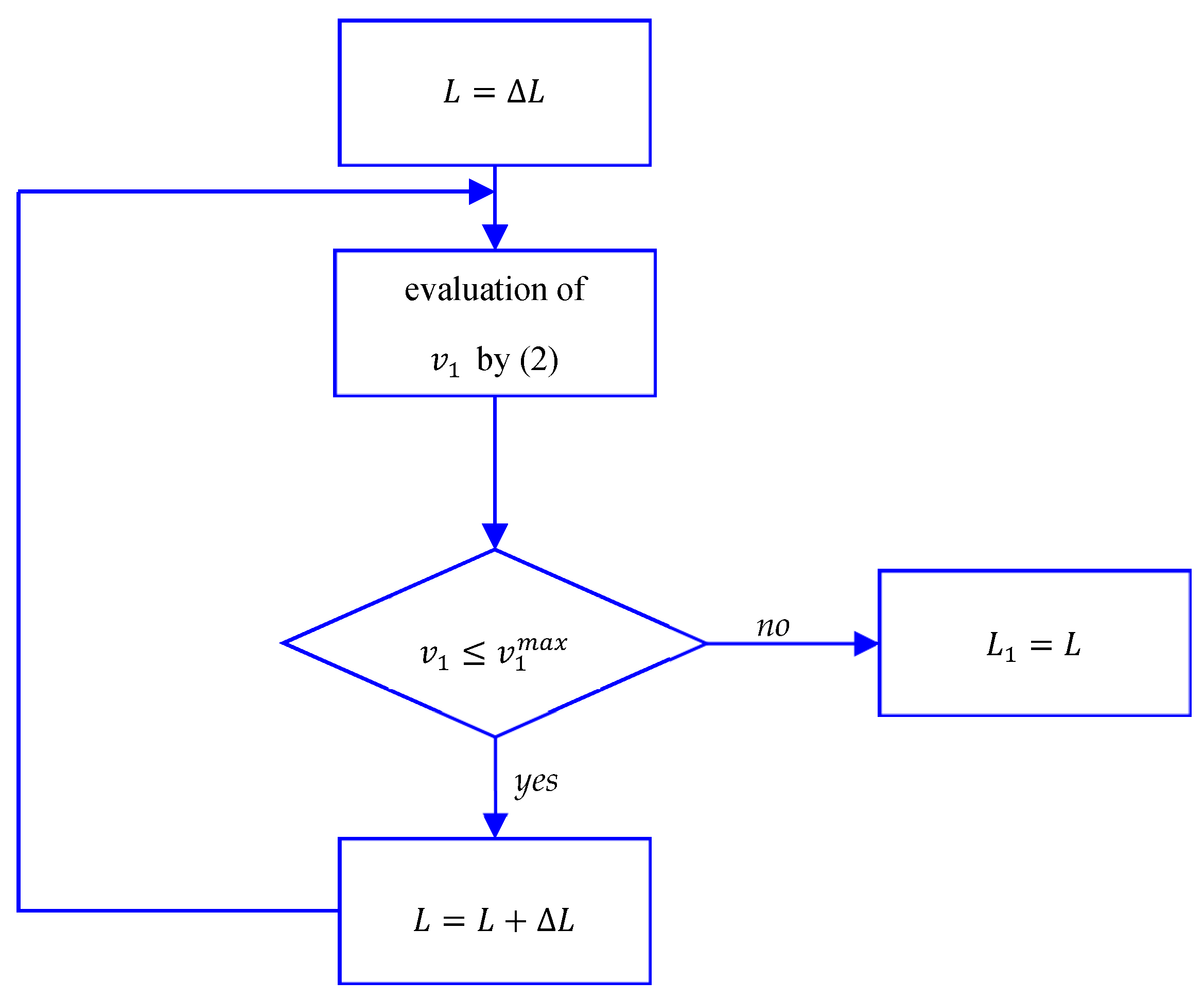
Practical evaluation of the first region of the loadability curve can be made through the simple iterative procedure reported in Figure 1, where $\Delta L$ is the length step (for example, it could be assumed $\Delta L=1\mathrm{km}$). It is sufficient to verify, for increasing values of $L$, that $v_1\le v_1^{max}$. The length $L_1$ is identified when the upper limit $v_1=v_1^{max}$ is attained. Of course, for $L\le L_1$ the maximum transmissible power $p\left(L\right)$ is equal to $p_{th}=a_{th}\cos {\phi }_2$, and does not change with the line length.

Section 4 shows the application of this procedure in a practical case.

The analytic solution is less immediate. For any assigned type of line and having set $\Delta v_{max}$, Equation (3) can be interpreted as a nonlinear equation in the unknown $L_1$. In Appendix A, an easy way to get an analytical solution of Equation (3) in the unknown $L_1$ is illustrated.

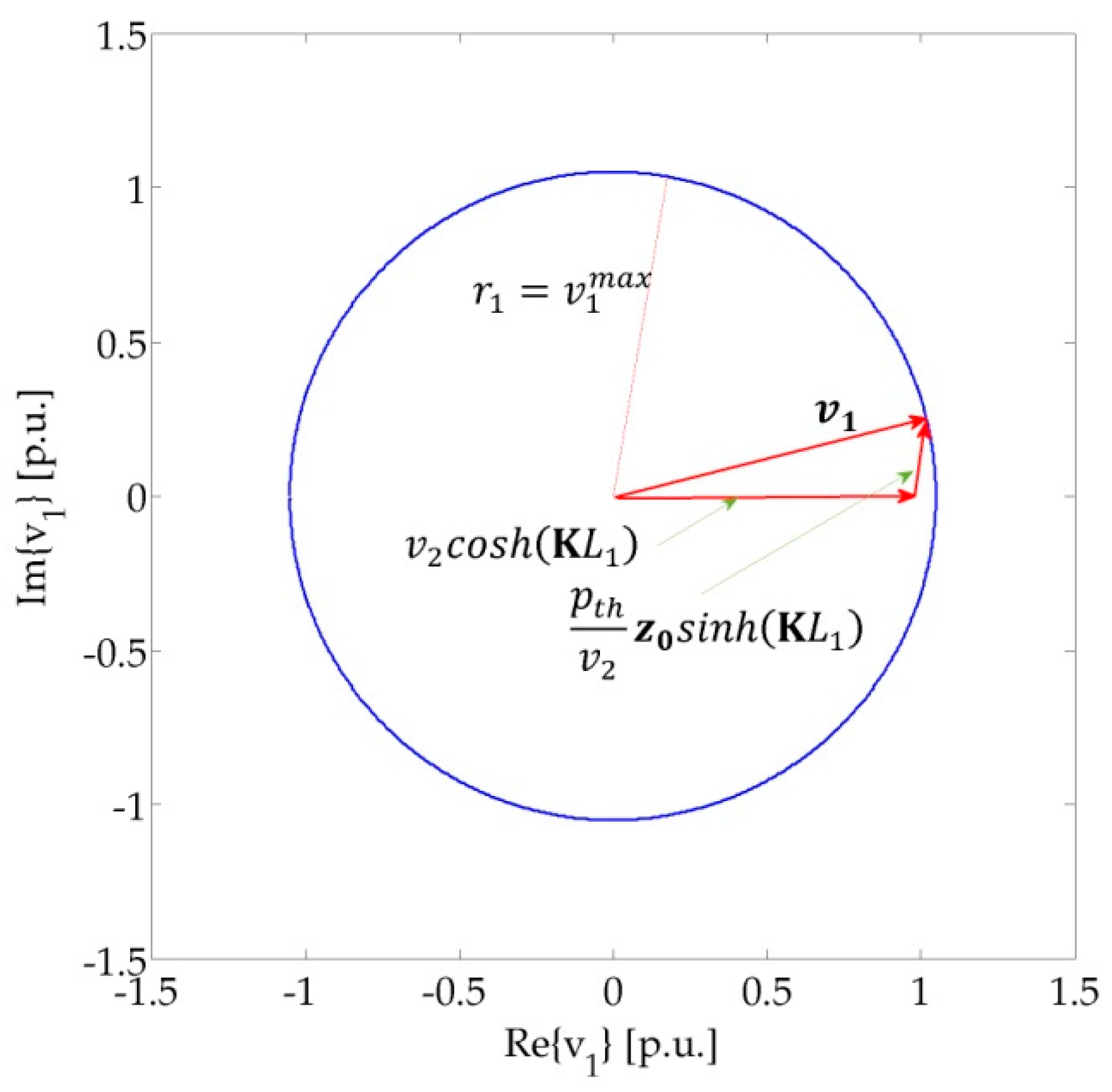
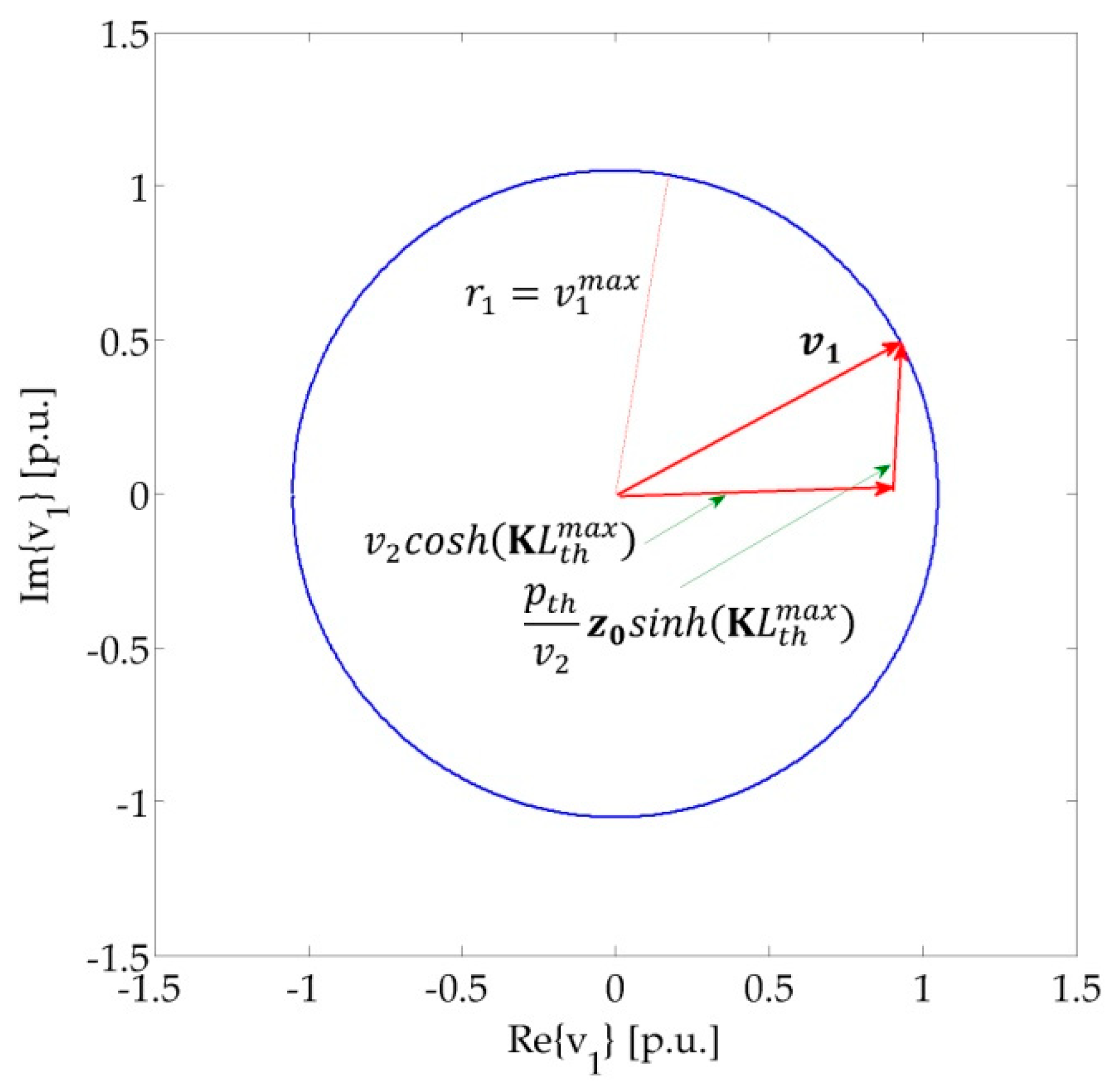
The well-known Perryne–Baum diagram is a helpful graphical representation of transmission lines steady-state operation. Figure 2 depicts in Cartesian coordinates the meaning of the relationship of Equation (3), for the base-case $cos{\phi }_2=1$. By adding the two phasors $v_{2}cosh\left(K{L}_1\right)$ and $\frac{p_{th}}{v_2}{\mathit{z}}_{\mathbf{0}}sinh\left(K{L}_1\right)$, the resulting vector $v_1$ intercepts the circle whose centre is located in the origin of the Cartesian coordinates system and whose radius is equal to $v_1^{max}=v_2+\Delta v_{max}$.

2.2. Voltage Drop Limit

The voltage drop limit affects the second region of the loadability curve, for $L>L_1,$ and until a different limit takes over. In this region, the maximum transmissible active power $p\left(L\right)$ (clearly, $p<p_{th}$) can be obtained by solving the equation

$$v_1^{max}=\left|v_{2}cosh\left(KL\right)+\frac{p}{v_2}\left(1-jtan{\phi }_2\right){\mathit{z}}_{\mathbf{0}}sinh\left(KL\right)\right|,$$

(4)

More easily, the unknown $p$ can be determined by solving the following algebraic quadratic equation, which can be derived properly rewriting Equation (4):

$$p^2\left({\gamma }^2+{\delta }^2\right)+2p\left(\alpha \gamma +\beta \delta \right)+{\alpha }^2+{\beta }^2-v_1^{max}{}^2=0,$$

(5)

where

$$\alpha =v_{2}cosh\left(K^{\prime }L\right)cos\left(K^{″}L\right),$$

(6)

$$\beta =v_{2}sinh\left(K^{\prime }L\right)sin\left(K^{″}L\right),$$

(7)

$$\gamma =\frac{1}{v_2}\left(\left(z_r+z_{y}tan{\phi }_2\right)sinh\left(K^{\prime }L\right)cos\left(K^{″}L\right)-\left(z_y-z_{r}tan{\phi }_2\right)cosh\left(K^{\prime }L\right)sin\left(K^{″}L\right)\right),$$

(8)

$$\delta =\frac{1}{v_2}\left(\left(z_r+z_{y}tan{\phi }_2\right)cosh\left(K^{\prime }L\right)sin\left(K^{″}L\right)+\left(z_y-z_{r}tan{\phi }_2\right)sinh\left(K^{\prime }L\right)cos\left(K^{″}L\right)\right).$$

(9)

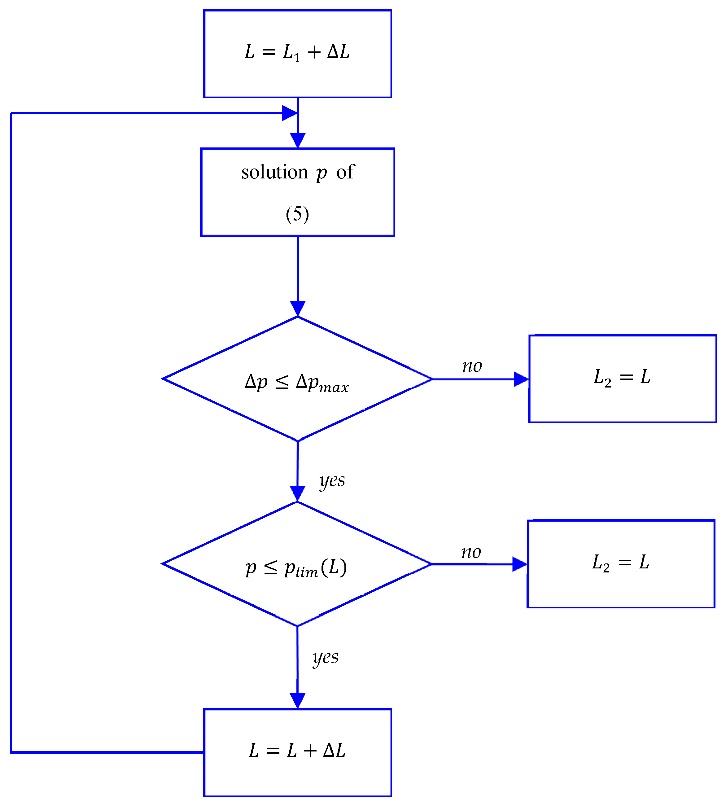
Therefore, the second region of the loadability curve $p\left(L\right)$ can be directly calculated solving Equation (5) in the unknown $p$ for each value of $L$ (with $L>L_1$). Once $p$ is obtained, it must be verified that the power losses and steady-state stability limits are not attained (the analytical description of these limits is reported in Section 2.3 and Section 2.4 below). The attainment of one of these limits determines the upper length of the second region of the loadability curve, $L_2$. This simple procedure is depicted in Figure 3.

Section 4 shows the application of this simple iterative procedure in a practical case.

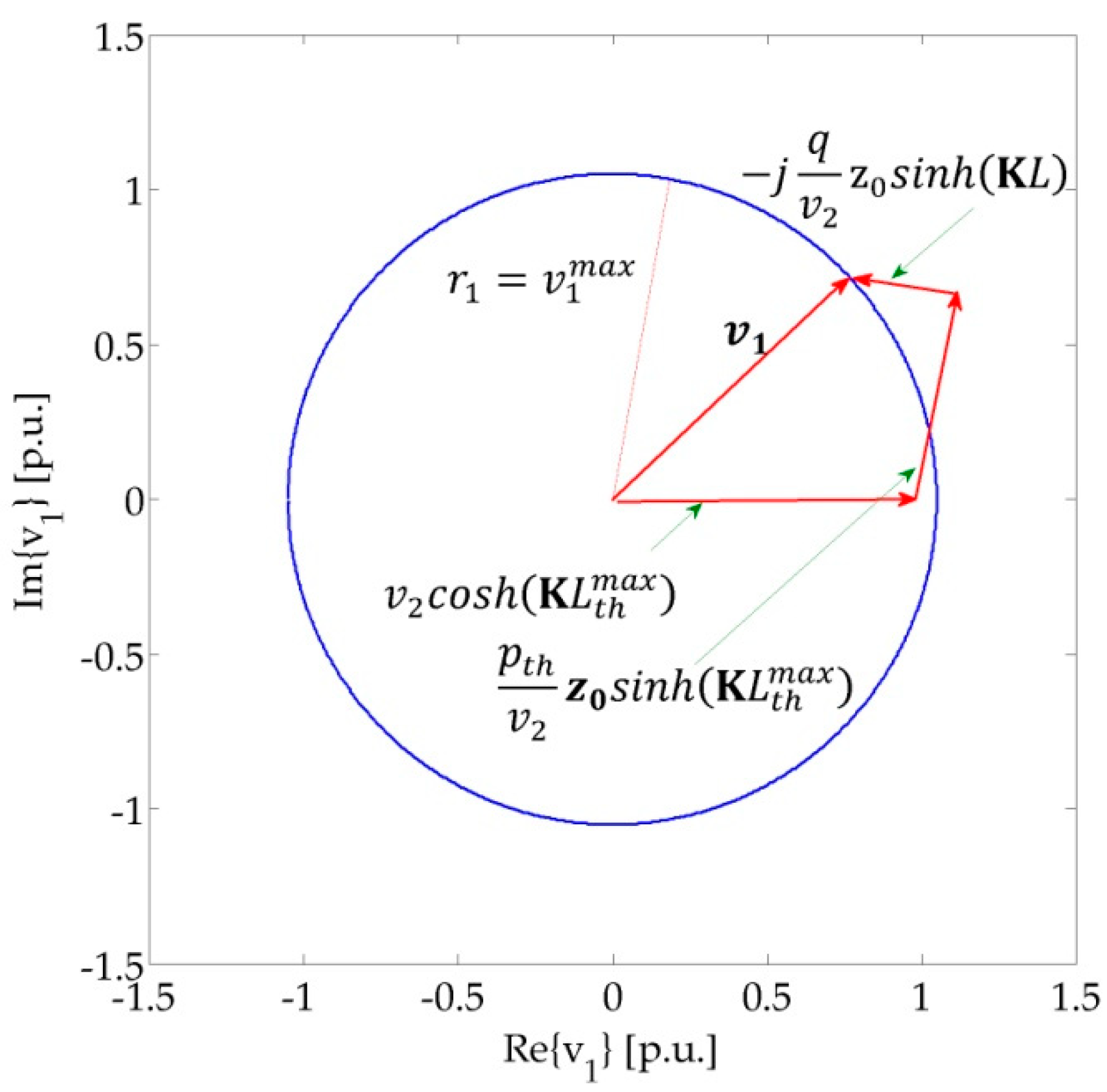
Referring to the Perryne–Baum diagram, $p$ can be interpreted as the value that intercepts the circle with radius $v_1^{max}$, as shown in Figure 4 with reference to the case $cos{\phi }_2=1$. Note that the two phasors $v_{2}cosh\left(KL\right)$ and $\frac{p}{v_2}\left(1-jtan{\phi }_2\right){\mathit{z}}_{\mathbf{0}}sinh\left(KL\right)$ vary with $L$ and, hence, have different values from those depicted in Figure 2.

2.3. Power Losses Limit

Concerning Joule losses along the line and considering that this paper deals with the maximum permissible power $p\left(L\right)$, a natural approach could be to fix a limit to the power losses $\Delta p$ calculated with regard to the loadability limit $p\left(L\right).$ Better, looking for homogeneity with the percent voltage drop limit, we could fix a limit to the ratio between $\Delta p$ and $p\left(L\right)$.

Analytically, considering that $p\left(L\right)$ must be intended as known (see Figure 3), this ratio can be calculated, for any given length $L$, as

$$\frac{\Delta p\left(p,L\right)}{p\left(L\right)}=\frac{Re\left\{{\mathit{v}}_{\mathbf{1}}{\mathit{i}}_{\mathbf{1}}{}^{*}\right\}}{p}-1$$

(10)

with

$$\begin{array}{c}{\mathit{v}}_{\mathbf{1}}=\mathit{A}{v}_2+\mathit{B}\frac{p}{v_2}\left(1-jtan{\phi }_2\right),\\ {\mathit{i}}_{\mathbf{1}}=\mathit{C}{v}_2+\mathit{A}\frac{p}{v_2}\left(1-jtan{\phi }_2\right).\end{array}$$

(11)

As we show in Appendix B, the ratio $\frac{\Delta p}{p\left(L\right)}$ can be explicitly evaluated as a function of $p$ and $L$.

From the methodological point of view, however, the problem is to identify a significant criterion for setting a limit to the ratio $\frac{\Delta p}{p\left(L\right)}$. Joule losses are an economic problem rather than a distinct limiting factor in line loadability. Thus, any limit concerning Joule losses should involve the energy $E_J$ lost in a given time period $T$ (for example, one year), whereas the instantaneous power losses corresponding to a certain power transported have scarce or no practical meaning [3,8,14].

It is clear that a limit on the lost energy $E_J^{max}$ is equivalent to a limit on the average value $p_m$ of the power transported. Thus, the load factor of the line $f_c=\frac{p_m}{p}$, i.e., the ratio between the average and the maximum power transported (in what follows, we assume the maximum power transported equal to $p\left(L\right))$ becomes a crucial parameter.

On the other hand, the ratio $f_p$ of the power losses $\Delta p_m$ evaluated with respect to $p_m$ and the power losses $\Delta p$ evaluated with regard to the maximum power $p\left(L\right)$, can be deduced from the load factor $f_c$ using the formula [15]:

$$f_p=\frac{\Delta p_m}{\Delta p}=0.7f_c^2+0.3f_c.$$

(12)

All this considered, we set a limit to the ratio $\frac{\Delta p_{\mathrm{m}}}{p_m}$, where $\Delta p_m$ is the power losses calculated with regard to the average power $p_m$. Finally, using Equation (12) and the definition of $f_c$, we can write

$${\left(\frac{\Delta p}{p\left(L\right)}\right)}^{max}={\left(\frac{\Delta p_m}{p_m\left(L\right)}\right)}^{max}\frac{f_c}{f_p}.$$

(13)

Equation (13) allows to calculate the maximum value of the ratio $\frac{\Delta p}{p\left(L\right)}$, as a function of the limit ${\left(\frac{\Delta p_m}{p_m\left(L\right)}\right)}^{max}$ and the load factor $f_c$. Therefore, once the load factor $f_c$ and the limit ${\left(\frac{\Delta p_m}{p_m\left(L\right)}\right)}^{max}$ are set, one can obtain ${\left(\frac{\Delta p}{p\left(L\right)}\right)}^{max}$ and check the constraint $\frac{\Delta p}{p\left(L\right)}\le {\left(\frac{\Delta p}{p\left(L\right)}\right)}^{max}$.

This procedure converts a limit to the lost energy into a limit to the (instantaneous) power losses $\Delta p$, calculated with regard to the loadability limit $p\left(L\right).$ Examples of application are shown in Section 4.

2.4. Steady-State Stability Limit

The stability limit depends not only on the transmission line characteristics, but also on the network equivalents at both line ends [6,7,8].

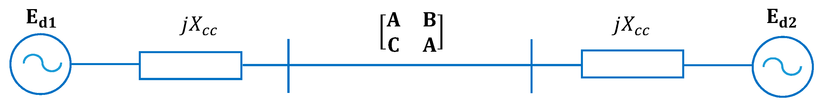
As far as the steady-state stability limit $p_{lim}$ is concerned, one can refer to the equivalent system shown in Figure 5.

The cascade system in Figure 5 can be described by the equivalent transmission matrix $\mathit{T}$:

$$\mathit{T}=\left[\begin{array}{cc}1& j{X}_{cc}\\ 0& 1\end{array}\right]\left[\begin{array}{cc}A& B\\ C& A\end{array}\right]\left[\begin{array}{cc}1& j{X}_{cc}\\ 0& 1\end{array}\right]=\left[\begin{array}{cc}{A}_t& B_t\\ C_t& A_t\end{array}\right].$$

(14)

The active power, expressed in p.u., is given by the well-known formula

$$p=\frac{e_{d1}{e}_{d2}}{b_t}cos\left({\beta }_t-\delta \right)-\frac{A_t{e}_{d2}^2}{b_t}cos\left({\beta }_t-{\alpha }_t\right),$$

(15)

where ${\mathit{b}}^{\mathit{t}}=b^t{e}^{j{\beta }_t}$ and ${\mathit{A}}^{\mathit{t}}=A^t{e}^{j{\alpha }_t}$.

The maximum value of $p$ is obtained for $\delta ={\beta }_t$, and is:

$$p_{max}=\frac{e_{d1}{e}_{d2}}{b_t}-\frac{A_t{e}_{d2}^2}{b_t}cos\left({\beta }_t-{\alpha }_t\right).$$

(16)

The steady-state stability limit $p_{lim}$ and $p_{max}$ are related each other by means of the stability margin $m_{stab}$, that is:

$$p_{lim}=\left(1-m_{stab}\right)\left(\frac{e_{d1}{e}_{d2}}{b_t}-\frac{A_t{e}_{d2}^2}{b_t}cos\left({\beta }_t-{\alpha }_t\right)\right).$$

(17)

This relationship is a monotonically decreasing function of $L$, $p_{lim}\left(L\right)$. For well-developed power systems, a good approximation of $p_{lim}$ is obtained assuming $e_{d1}=v_1^{max}$ and $e_{d2}=v_2$. In this case, Equation (17) becomes

$$p_{lim}\left(L\right)=\left(1-m_{stab}\right)\left(\frac{v_1^{max}{v}_2}{b_t\left(L\right)}-\frac{A_t\left(L\right)v_2^2}{b_t\left(L\right)}cos\left({\beta }_t\left(L\right)-{\alpha }_t\left(L\right)\right)\right).$$

(18)

The maximum allowable active power, therefore, must satisfy the inequality:

$$p\left(L\right)\le p_{lim}\left(L\right).$$

(19)

According to the procedure illustrated in Figure 3, the inequality (19) must be checked for each value of $L$. In this case also, Section 4 shows the application of this procedure in a practical case.

2.5. Third Region of The Loadability Characteristic

At the line length $L_2$ either the power losses or the steady-state stability limit is attained. Longer lines ($L>L_2$) belong to further regions of the loadability curve. Obviously, the third region is determined by the limit attained (power losses or steady-state stability). Examples reported in Section 4 show that $L_2$ is usually quite long and, thus, the majority of the existing OHLs belong to the first two regions.

3. Analytical Formulation of Loadability Characteristics for Shunt Compensated Radial Lines

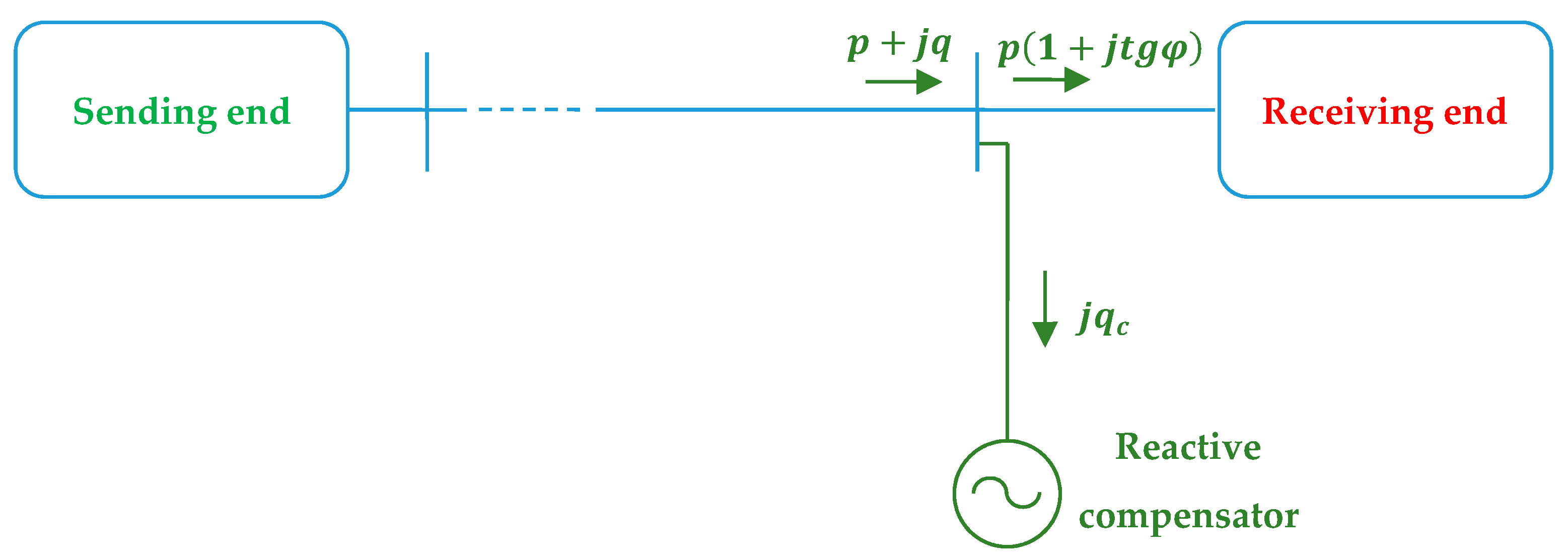
Referring to the specific case of radial OHLs with shunt reactive compensation at the receiving end, is illustrated in Figure 6. The shunt compensation (reactive power injection $q_c<0$) superimposes a backward (i.e., from the receiving end to the sending end) reactive power flow to the forward active power flow. Assuming $cos{\mathsf{\phi }}_2=1$, it follows $q=q_c<0$. In this way the voltage drop across the line can be limited and, thus, the power transfer capacity increases. This operation is illustrated in Figure 7.

Accordingly, reactive compensation is useful to increase the loadability curve in the second region, whereas in the thermal limit region a reactive power injection would reduce the loadability limit $\left(L\right)=$ $p_{th}$.

Some preliminary considerations help to understand the succession of the various limits in the loadability curve of these lines. Unlike uncompensated OHLs, in this case the slight difference between the modulus of the sending end and receiving end currents plays a role in deriving the loadability characteristics. Until the voltage drop is less than $\mathsf{\Delta }{v}_{max}$, as already said in Section 2.1, the modulus of the current at the sending end is slightly lower than that at the receiving end, which is equal to the thermal limit. Once the voltage drop limit is achieved, the modulus of the current at the sending end increases with $L$ until, at a certain length $L_2$, it attains the thermal limit and equals the receiving-end current. After this length, not to exceed the thermal limit the compensation action must decrease. These aspects are quantified in the practical example discussed in Section 4.2.

Keeping this in mind, the succession of the various limits and the relevant analytical description are explained in the following subsections where, for the sake of clarity, the case of unitary power factor is examined first.

3.1. Receiving-End Thermal Limit

It is trivial to remark that, until the voltage drop limit is achieved, reactive compensation is not required and the loadability curve coincides with that of uncompensated lines. Hence, the maximum line length for which reactive compensation is not required, is equal to $L_1.$

3.2. Receiving-End Thermal Limit and Voltage Drop Limit

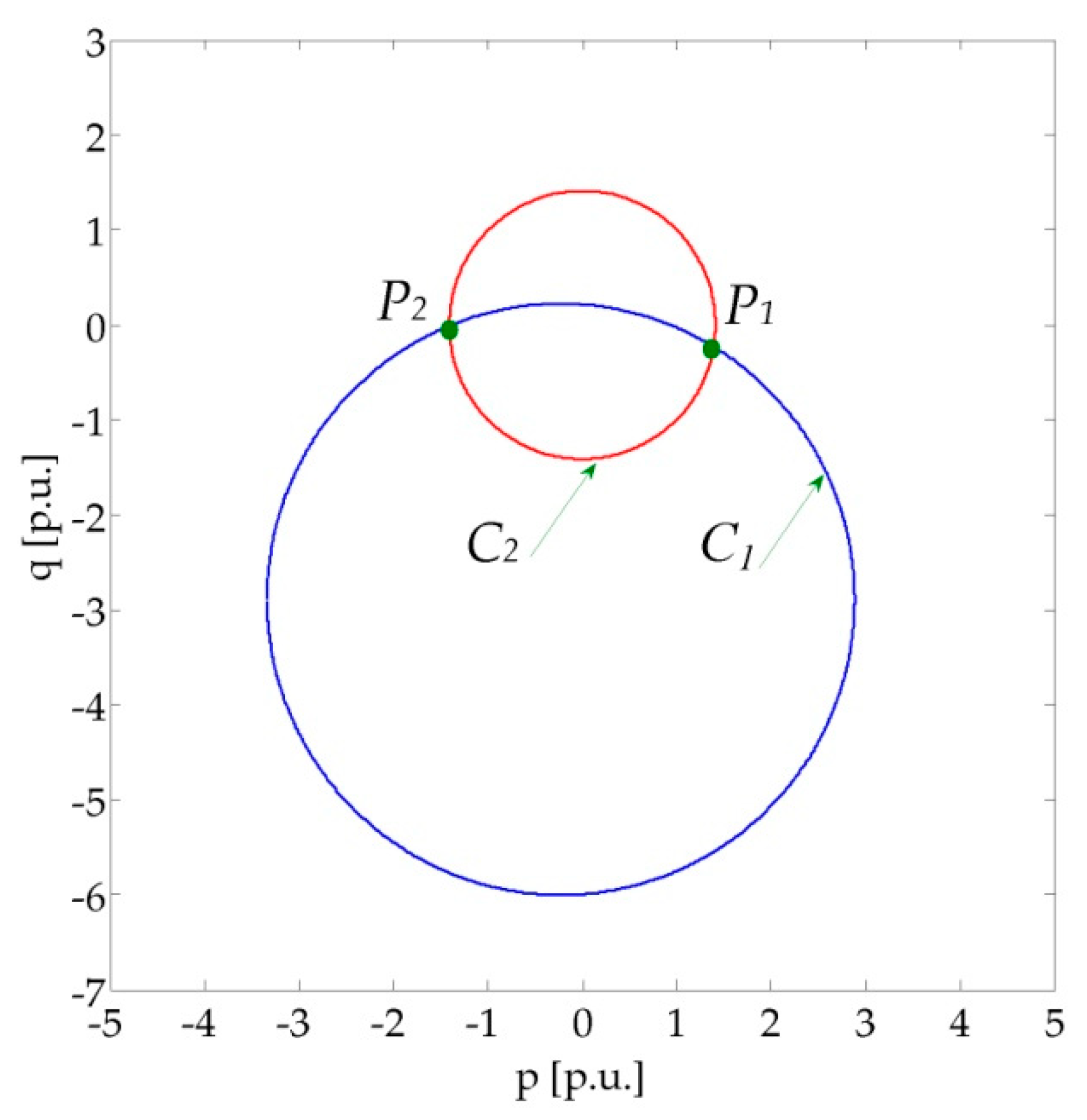
The voltage phasor diagram shown in Figure 7 is characterized by the following equations:

$$\begin{array}{c}{v}_1^{max}={\left|v_2\cos h\left(KL\right)+\frac{p-jq}{v_2}{z}_{0}sinh\left(KL\right)\right|}_{L>L_1}\\ \sqrt{p^2+q^2}=a_{th}.\end{array},$$

(20)

For each value of $L$ (and, thus, for any given line), the two relationships in Equation (20) represent the two power circles, C₁ and C₂, shown in Figure 8, and expressed in Cartesian coordinates $\left(p,q\right)$ as

$$\{\begin{array}{c}{\left(p-p_1\right)}^2+{\left(q-q_1\right)}^2=r_1^2\\ {\left(p-p_2\right)}^2+{\left(q-q_2\right)}^2=r_2^2\end{array},$$

(21)

where

$$\begin{gathered} p_1=-Re\left\{{\left(\frac{v_2^2\cos h\left(KL\right)}{{\mathrm{z}}_{0}sinh\left(KL\right)}\right)}^{*}\right\},q_1=-Im\left\{{\left(\frac{v_2^2\cos h\left(KL\right)}{{\mathrm{z}}_{0}sinh\left(KL\right)}\right)}^{*}\right\},\mathrm{and}{r}_1=\frac{v_1^{max}{v}_2}{\left|z_{0}sinh\left(KL\right)\right|}, \\ {p}_2=0,q_2=0,r_2=a_{th}, \end{gathered}$$

(22)

The points of intersection of the circles in Equation (21) are P₁ and P₂ in Figure 8. The maximum allowable active power $p\left(L\right)$ corresponds to the abscissa of P₁, whose coordinates are obtained by solving Equation (21). For this purpose, as is well known from analytical geometry, the radical axis, i.e., the line passing through $P_1$ and $P_2$, is described by the equation:

$$q=-\frac{p_2-p_1}{q_2-q_1}p+\frac{p_2^2-p_1^2+q_2^2-q_1^2+r_1^2-r_2^2}{2\left(q_2-q_1\right)}$$

(23)

Hence, by substituting Equation (23) in one of the formulas in Equation (21), the coordinates of P₁ and P₂ can be derived. In this way, $p\left(L\right)$ can be obtained for each line length $L$ (with $L>L_1$).

This simple analytical procedure (similar in principle to that illustrated in Figure 3) allows calculation of the second region of the loadability curve.

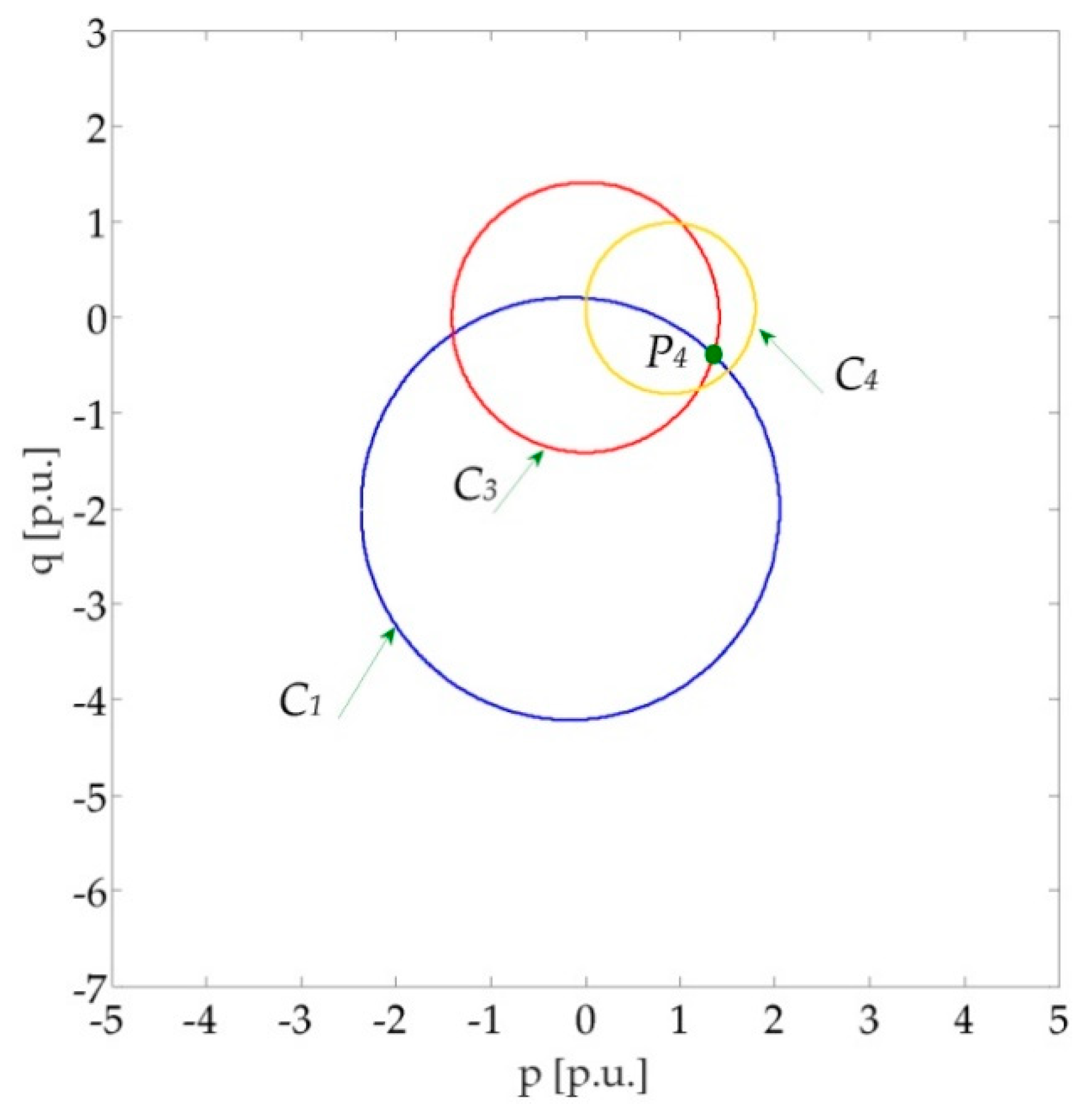
The second region extends up to the line length at which another limit is attained. Therefore, as made above for uncompensated lines, the attainment of another limit must be checked. In this case, the check concerns the attainment of the thermal limit at the sending end at the length $L_2$. As already said, at this line length the currents at the two line ends are both equal to the thermal limit. Analytically, at $L_2$ the following constraints are attained at the same time:

$$\begin{array}{c}\sqrt{p^2+q^2}=a_{th},\\ v_1^{max}=\left|cosh\left(\mathit{K}{L}_2\right)+\frac{p-jq}{v_2}{\mathit{z}}_{\mathbf{0}}sinh\left(\mathit{K}{L}_2\right)\right|\\ \left|\frac{v_2}{{\mathit{z}}_{\mathbf{0}}}sinh\left(\mathit{K}{L}_2\right)+\frac{p-jq}{v_2}cosh\left(\mathit{K}{L}_2\right)\right|=i_{th}\end{array},$$

(24)

Also the third relationship of (24) can be represented by a circle, named C₃ and expressed in Cartesian coordinates $\left(p,q\right)$ as:

$${\left(p-p_3\right)}^2+{\left(q-q_3\right)}^2=r_3^2,$$

(25)

where:

$$p_3=-Re\left\{\frac{tgh\left(KL\right)}{z_{\mathbf{0}}}\right\},q_3=Im\left\{\frac{tgh\left(KL\right)}{z_{\mathbf{0}}}\right\},r_3=\frac{i_{th}}{\left|\cos \mathrm{h}\left(KL\right)\right|}$$

(26)

For $L=L_2$ the three circles C₁, C₂ and C₃, which are the geometrical representation of (21) and (25), have a common intersection point $P_3$, which identifies the maximum allowable active power, as shown in Figure 9.

In order to determine the coordinates of $P_3$ avoiding the complex solution of the system (24), it is convenient to resort to an iterative procedure similar in principle to those described in Figure 1 and Figure 3. The module of the sending end current can be calculated, for increasing values of $L$, using the left-hand member of the first of (24): the point $P_3$ is identified when the sending end current attains the thermal limit. Section 4 shows the application of this procedure in a practical case.

3.3. Sending-End Thermal Limit and Voltage Drop Limit

When the thermal limit is attained at the sending end, the maximum allowable active power $p\left(L\right)$can be calculated by solving the following two-equations system:

$$\begin{array}{c}{v}_1^{max}={\left|v_{2}cosh\left(KL\right)+\frac{p-jq}{v_2}{z}_{0}sinh\left(KL\right)\right|}_{L>L_2}\\ {\left|\frac{v_2}{{\mathrm{z}}_0}sinh\left(KL\right)+\frac{p-jq}{v_2}cosh\left(KL\right)\right|}_{L>L_2}=i_{th}\end{array}.$$

(27)

In this way, a third region of the loadability curve can be calculated, likewise we already performed in Section 3.2 with regard to the second region. Indeed, for each value of $L$ (with $L>L_2$) the system in Equation (27) can also be reduced to a system of two algebraic quadratic equations.

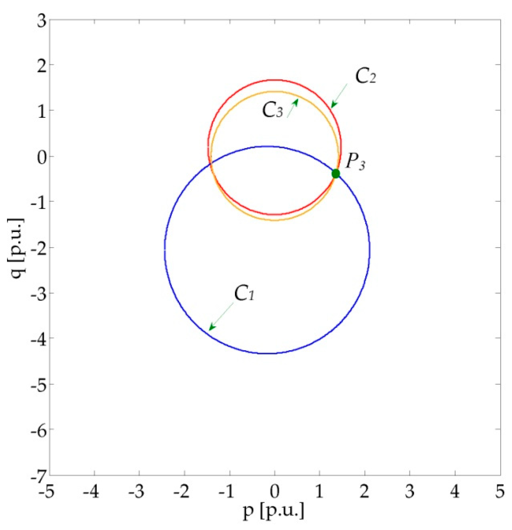
The solution of Equation (27) is graphically represented by the intersection of the circles C₁ and C₃ illustrated in Figure 10. Clearly, the maximum allowable active power is determined by the intersection point $P_4$ of C₁ and C₃.

The figure reports also the circle C₄ that represents the power losses limit. This limit, indeed, can be written as

$${\left(p-p_4\right)}^2+{\left(q-q_4\right)}^2=r_4^2$$

(28)

with $p_4$, $q_4$ and $r_4$ given by

$$p_4=-\frac{v_2^2\left(A^2+Re\left\{B{C}^{*}\right\}-\left(1+\Delta p_{max}\right)\right)}{2Re\left\{A^{*}B\right\}},q_4=-\frac{v_2^{2}Im\left\{B{C}^{*}\right\}}{2Re\left\{A^{*}B\right\}},\mathrm{and}{r}_4=\sqrt{p_4^2+q_4^2-\frac{v_2^{4}Re\left\{A{C}^{*}\right\}}{Re\left\{A^{*}B\right\}}}$$

(29)

Equation (28) corresponds to the circle C₄ depicted in Figure 10.

In practice, in order to check satisfaction of the power losses limit, once the solution $p^{*}\left(L\right)$, $q^{*}\left(L\right)$ of Equation (27) is obtained, it must be verified that this point is within the circle C₄, i.e., ${\left(p^{*}\left(L\right)-p_4\right)}^2+{\left(q^{*}\left(L\right)-q_4\right)}^2<r_4^2$. In the same way, one can simply verify, for each value of $L$, the satisfaction of the steady-state stability limit (19) that can be rewritten, by assuming infinite short-circuit power at both line ends, i.e., $e_{d1}=v_1^{max}$ and $e_{d2}=v_2$, as

$$p^{*}\left(L\right)\le \frac{\left(1-m_{stab}\right)}{b\left(L\right)}\left(v_1^{max}{v}_2-A\left(L\right)v_2^{2}cos\left(\beta \left(L\right)-\alpha \left(L\right)\right)\right).$$

(30)

A practical example of application is shown in Section 4.

3.4. Voltage Drop Limit and Steady-State Stability Limit

For longer lines, starting from a certain line length $L_3$, the steady-state stability limit starts determining the loadability curve (note that, in compensated lines, this line length can be much lower compared with the base-case of uncompensated lines). Thus, the loadability limit is determined by the voltage drop and steady-state stability limits. In this region, both the active and reactive power of the compensator decrease starting from the maximum value of complex power. If the maximum reactive power the synchronous condenser can deliver, $Q_{max}$, is less than this value, the sequence of the limits can change.

Analytically, for $L>L_3$, the maximum active power is calculated as

$$p_{lim}\left(L\right)=\frac{\left(1-m_{stab}\right)}{b\left(L\right)}\left(v_1^{max}{v}_2-A\left(L\right)v_2^{2}cos\left(\beta \left(L\right)-\alpha \left(L\right)\right)\right).$$

(31)

The reactive power $q$ in turn can be calculated by solving the following relationship:

$$v_1^{max}={\left|\cos h\left(KL\right)+\frac{p_{lim}-jq}{v_2}{z}_{\mathbf{0}}\sin h\left(KL\right)\right|}_{L>L_3}$$

(32)

Equation (32) can also be reduced to a second order algebraic equation in the unknown $q$, following the same procedure already shown for Equation (4). For the sake of brevity, the relevant equations are not reported here.

3.5. $Case:cos{\phi }_2\ne 1$

The more general case with $cos{\mathsf{\phi }}_2\ne 1$ can be reduced to the case $cos{\mathsf{\phi }}_2=1$ by adding a further reactive compensation $q_c=-Ptan{\phi }_2$. This means that the whole reactive power absorbed by the load is delivered by the synchronous condenser and the line power factor at the receiving end of the line, ${\cos \mathsf{\phi }}_2$, is adjusted to 1. This, of course, requires $Q_{max}>Ptan{\mathsf{\phi }}_2$ and implies that a reduced reactive power reserve, equal to $Q_{max}-Ptan{\phi }_2$, is available to control the voltage drop across the line.

4. Practical Applications

The goal of this Section is to show the ability of the proposed analytical methodology to derive the loadability characteristic of OHLs. Calculations are performed for the base-case of uncompensated OHLs and for the specific case of shunt compensated radial lines. In the second case, we assume that a synchronous condenser is connected at the receiving end of the OHL, as shown in Figure 6. The limits considered in both cases are:

• conductor thermal limit, $i_{th}$;
• voltage drop limit, $\Delta v_{max}$;
• power losses limit, ${\left(\frac{\Delta p_m}{p_m\left(L\right)}\right)}^{max}$; and
• steady-state stability limit, $m_{stab}$.

Calculations concern traditional single circuit 400 kV OHLs equipped with a standard triple-core ACSR conductor bundle of 3 × 585 mm² cross section, already taken as reference conductors in [6,7]. The relevant line parameters are reported in

Table 1. Per unit length line parameters.

Parameter	Unit	Value
Resistance, $r$	$\mathsf{\Omega }/\mathrm{km}$	0.021
Reactance, $x$	$\mathsf{\Omega }/\mathrm{km}$	0.271
Conductance, $g$	$\mathrm{S}/\mathrm{km}$	4 × 10−9
Susceptance, $b$	$\mathrm{S}/\mathrm{km}$	4.21 × 10−6

.

The values in Table 1 yield to ${\mathit{Z}}_{\mathbf{0}}=Z_r+j{Z}_y=253.90-j9.83\mathsf{\Omega },\mathit{K}=K^{\prime }+jK{}^{″}$ = $4.186\times {10}^{-5}+j1.068\times {10}^{-3}$and SIL $=620\mathrm{MW}$. At the receiving end it is set $v_2=1\mathrm{p}.\mathrm{u}.$ and the thermal limit is assumed as $I_{th}=2038\mathrm{A}$ (according to the Italian Standard CEI 11-60 [16], the conductor thermal limit $I_{th}$ ranges from 2038 to 2952 A depending on the season and geographical location. Here, we take the lowest—most conservative—value of $I_{th}$= 2038 A), which corresponds to $A_{th}=1412$ $\mathrm{MVA}$.

The percent value of maximum voltage drop is assumed $\Delta v_{max\%}=5\%$.

With regard to Joule losses, we assume ${\left(\frac{\Delta p_m}{p_m\left(L\right)}\right)}^{max}=$ 5%, and a load factor $f_c=0.75$. The last assumption is rather conservative, as it corresponds to a rather high average exploitation of the line. From (12) we obtain $f_p=0.619$ and, from (13), ${\left(\frac{\Delta p}{p\left(L\right)}\right)}^{max}=0.0606\mathrm{p}.\mathrm{u}.$

With regard to the steady-state stability margin, the commonly used value of 30% $(m_{stab}=0.3)$is considered. Finally, regarding the power factor, the case $cos{\phi }_2=1$ is analyzed first.

Using these values and the relationships explained in Section 2 and Section 3, it is rather easy to calculate the loadability curves of both uncompensated and compensated lines.

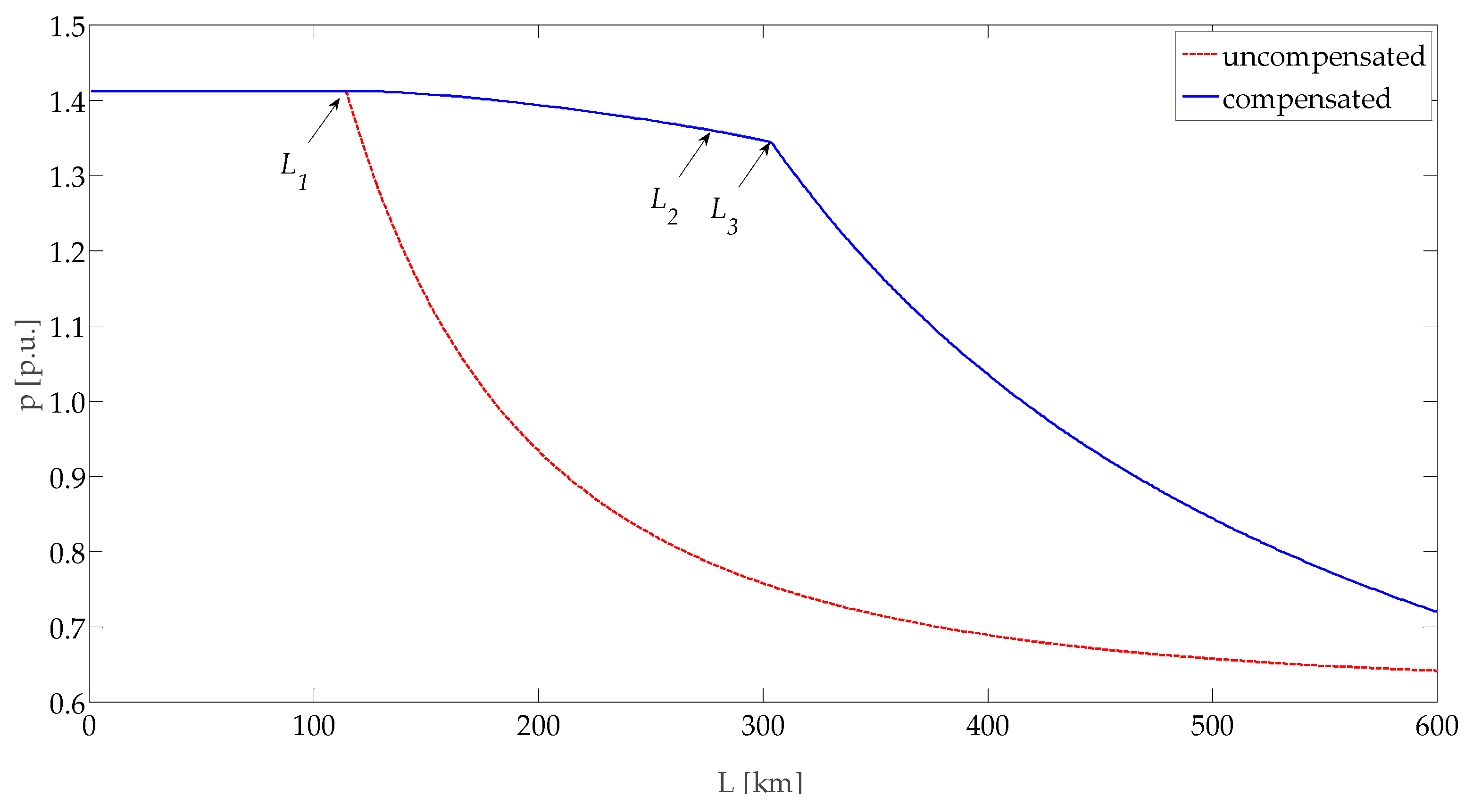
Figure 11 shows the loadability curves obtained with $v_2=1$. On the y-axis, powers are in $\mathrm{p}.\mathrm{u}.$ of a 1000 MVA base power.

4.1. Uncompensated Lines

The numerical solution (illustrated in Figure 1) of the non-linear Equation (3) provides $L_1=114\mathrm{km},$ whereas the approximated analytical solution described in Appendix B gives 118 km. However, this error dramatically reduces with the power factor and, at $cos{\phi }_2<0.97$, the difference between the numerical and analytical solutions practically vanishes.

Hence, the first region of the loadability curve has constant ordinate equal to $p_{th}$ in the length interval 0–114 $\mathrm{km}$.

The second region of the loadability curve is calculated by solving Equation (4) in the unknown variable $p$ for each value of $L>L_1$. For these relatively long lines, the limit $\Delta v_{max\%}=5\%$ imposes to reduce the transmissible power and, increasing $L$, the line loadability $p\left(L\right)$ quickly decreases.

For each value of $p$, power losses can be evaluated by (A9), and the constraint $\frac{\Delta p}{p\left(L\right)}\le {\left(\frac{\Delta p}{p\left(L\right)}\right)}^{max}$ can be easily checked. The limit value ${\left(\frac{\Delta p}{p\left(L\right)}\right)}^{max}$ is never achieved at least until $L=600\mathrm{km}$. In fact, for $L=600\mathrm{km}$ the loadability limit, determined through Equation (5) where the numerical values of the parameters $\alpha$, $\beta$, and $\delta$ are $0.8015,0.0150,0.0687$, and $0.9721$ respectively, is $p=0.641\mathrm{p}.\mathrm{u}.$ The relationship (A7), reported in Appendix B, for $p=0.641\mathrm{p}.\mathrm{u}.$ and $L=600\mathrm{km}$ provides $\frac{\Delta p}{p\left(L\right)}=0.0529\mathrm{p}.\mathrm{u}.$ that is less than ${\left(\frac{\Delta p}{p\left(L\right)}\right)}^{max}=0.0606\mathrm{p}.\mathrm{u}.$

With regard to steady-state stability, having set $m_{stab}=0.3$ and assuming an infinite short-circuit-ratio at both line ends, until $L=600\mathrm{km}$ the steady-state stability limit does also not affect the line loadability. In fact, for $L=600\mathrm{km}$ the relationship in Equation (17) gives $p_{lim}=0.719\mathrm{p}.\mathrm{u}.$, higher than the power corresponding to $\Delta v_{max\%}$ ($0.641\mathrm{p}.\mathrm{u}.$).

In summary, for the considered OHLs the loadability curve calculated in the 0–600 km range of lengths consists of only two regions, resulting $L_2>600\mathrm{km}$. The limit length $L_1$ and the loadability curve $p\left(L\right)$ can be easily derived, as just illustrated, avoiding the need to resort to optimization procedures, which generally require a major effort for the implementation on a digital computer and more computation burden.

Note that, assuming different values for the power losses limit ${\left(\frac{\Delta p_m}{p_m\left(L\right)}\right)}^{max}$ and the load factor $f_c$, the Joule losses limit could prevail over the voltage drop limit reducing the loadability curve after a certain line length that can be individuated by the methodology described. The same is valid in the case of a more stringent setting of the steady-state stability limit.

4.2. Shunt Compensated Radial Lines

For shunt compensated radial lines, it is obvious that the first region of the loadability curve is equal to the one of uncompensated lines. Starting from the line length $L_1$, the injection of the required amount of reactive power allows limiting the voltage drop across the line and thus avoids exceeding the voltage drop limit $\Delta v_{max\%}=5\%$. Increasing $L$, this operation continues until other limits are attained or the reactive power reserve is fully exploited. As already pointed out, the second region of the loadability curve is determined by both the thermal limit at the receiving end and the voltage drop limit. This operation is graphically represented by the intersection point $P_1$ of the circles C₁ and C₂ illustrated in Figure 8, whose Cartesian coordinates are given by Equation (21). Analytically, the coordinates of $P_1$ must be determined. The maximum allowable active power corresponds to the abscissa of $P_1$, which is determined for each value of $L>L_1$ by solving the linear relationship in Equation (23) and one of the two Equations (21), as described in Section 3. The only computation effort required is the solution of a second order algebraic equation. For example, for $L=200\mathrm{km}$, the equations system becomes

$$\{\begin{array}{c}{\left(p+0.2274\right)}^2+{\left(q+2.8894\right)}^2=9.6970\\ q=-0.0787p-0.1206\end{array}.$$

(33)

Solving this system, the coordinates of $P_1$ are $p=1.393\mathrm{p}.\mathrm{u}.$ and $q=-0.230\mathrm{p}.\mathrm{u}.$ Note that the reactive power, which corresponds to a capacitive absorption, can be actually delivered only if it is lower than the rating of the synchronous condenser.

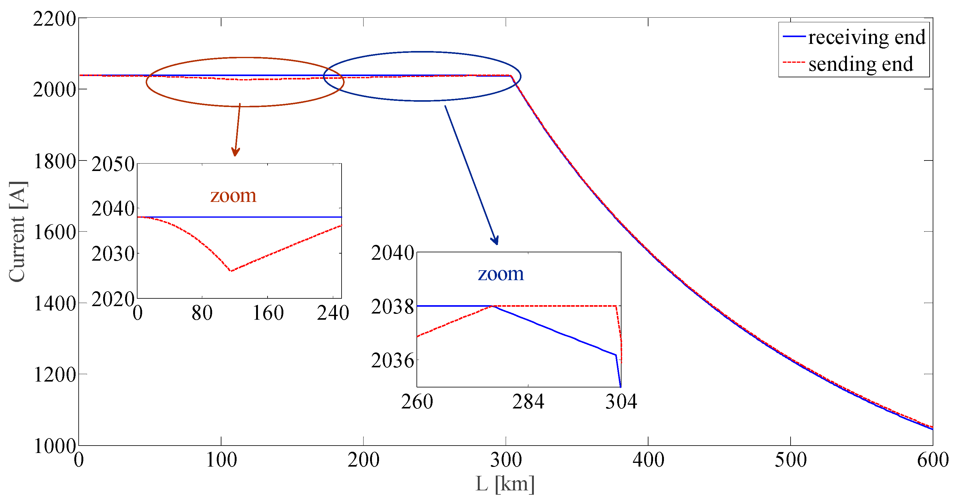
The second region extends up to the line length $L_2$at which also the sending end current achieves the thermal limit (Figure 12). This length corresponds to point $P_3$ depicted in Figure 9.

The numerical procedure explained at the end of Section 3.2 provides $L_2=276\mathrm{km}$, and the coordinates of $P_3$ are $p=1.356\mathrm{p}.\mathrm{u}$., and $q=-0.394\mathrm{p}.\mathrm{u}.$

The gradual and moderate reduction of the loadability curve (Figure 11) in the second region (114–276 $\mathrm{km})$ is due to the thermal limit and to the progressive reduction of the line power factor: The increasing reactive component of the current, injected for compensation, reduces the active current in the line.

After $L=276\mathrm{km}$, the third region is determined by the thermal limit at the sending end and by the voltage drop limit, and is analytically represented by Equation (27). For each value of $L$, the powers $p$ and $q$ can be evaluated as the intersection of the two circles C₁ and C₃ illustrated in Figure 10. It must be also verified that the power losses limit ${\left(\frac{\Delta p_m}{p_m\left(L\right)}\right)}^{max}$and the steady-state stability margin $m_{stab}$ are not exceeded. This can be done by means of Equations (28) and (30), respectively. For the specific case under study, the steady-state stability limit takes over at $L_3=304\mathrm{km}$. Indeed, at this length the maximum active power $p$ compatible with the thermal and voltage drop limits (obtained by the solution of (27)) is equal to the maximum active power $p^{*}\left(L\right)$ compatible with the steady-state stability limit (obtained by (30)): $p=p^{*}\left(L\right)=1.344\mathrm{p}.\mathrm{u}.$

Also in this case, the power losses limit is never attained. Indeed, for $L=600\mathrm{km}$, $\frac{\Delta p}{p\left(L\right)}=0.0590\mathrm{p}.\mathrm{u}.$ which is lower than ${\left(\frac{\Delta p}{p\left(L\right)}\right)}^{max}=0.0606\mathrm{p}.\mathrm{u}.$

Concluding, the explained calculations allow determining the loadability curve depicted in Figure 11, which is determined by the following sequence of limits:

• $L\le L_1$: Thermal limit at the receiving end;
• $L_1\le L\le L_2$: Voltage drop limit and thermal limit at the receiving end;
• $L_2\le L\le L_3$: Voltage drop limit and thermal limit at the sending end;
• $L_3\le L\le 600\mathrm{km}$: Voltage drop limit and steady-state stability limit.

with $L_1=114\mathrm{km}$, $L_2=276\mathrm{km},$ and $L_3=304\mathrm{km}$.

4.3. Case: $cos{\phi }_2<1$

In case of less than one load power factor (practical values can be assumed in the range (0.97–1), the loadability curve of uncompensated lines reduces because

• the active power transmitted at the thermal limit is proportional to $cos{\mathsf{\phi }}_2$; this causes a small loadability reduction in the first region; and
• the voltage drop across the line increases; this causes a much greater loadability reduction in the three following regions, all affected by the voltage drop limit.

Also, the limit length $L_1$ sharply reduces [6,7]. The analytical calculation of $L_1$ for $cos{\mathsf{\phi }}_2=0.97$, performed as explained in Appendix A, gives the value 58 km which is almost identical to the numerical solution obtained through widespread algorithms for the solution of nonlinear algebraic equations, such as Newton–Raphson. Practically the same result is obtained by means of the numerical solution illustrated in Figure 1. For example, assuming $\Delta L=1\mathrm{km}$, the result is $L_1=$59 km.

On the contrary, in the case of shunt compensated radial lines, the compensator action (provided that the compensator can provide the reactive power amount required to adjust to unity the load power factor) allows to obtain the same loadability curve reported in Figure 11 for the case ${\cos \mathsf{\phi }}_2=1$.

5. Conclusions

This paper proposes a new approach for the analytical description of the various regions of the loadability curves of overhead transmission lines. Using the complete line model with distributed parameters and the relevant general formulation, we show how the loadability curves of any actual line can be deduced taking into account the conductor thermal limit, a maximum voltage drop across the line, a maximum amount of Joule losses along the line, and a steady-state stability margin.

The analytical formulation has general validity and can be used to calculate the loadability curves—helping power system operators in both planning and operation stages—in all practical cases. The last sentence is demonstrated by two application examples. The first example refers to the base-case of standard (uncompensated) 400 kV single circuit OHLs equipped with standard triple-core ACSR conductor bundle with 3 × 585 mm² cross section, whereas the second example concerns the same 400 kV single circuit OHLs in radial topology and shunt compensated at the receiving end.

Despite the apparent complexity of the general analytical description, we demonstrate that the practical application of this analytical approach is rather simple. In both case studies, the loadability curves can be easily derived, avoiding the need to formulate the loadability problem in terms of a constrained optimization problem, whose solution implies an adequate procedure of implementation on a digital computer and a major computation burden.