Dispensing Technology of 3D Printing Optical Lens with Its Applications

Abstract
:
1. Introduction
2. Principle
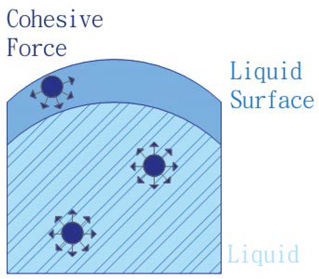
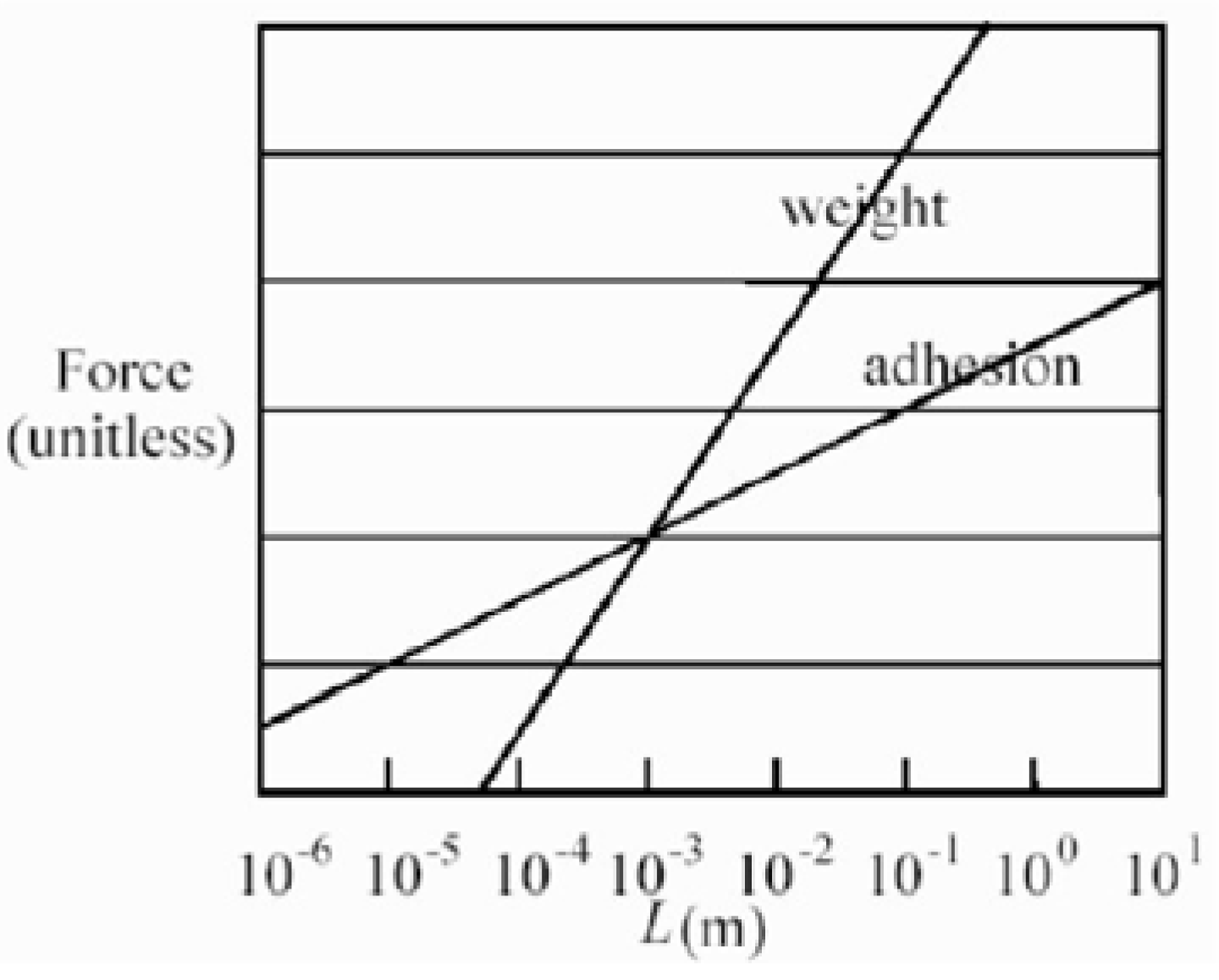
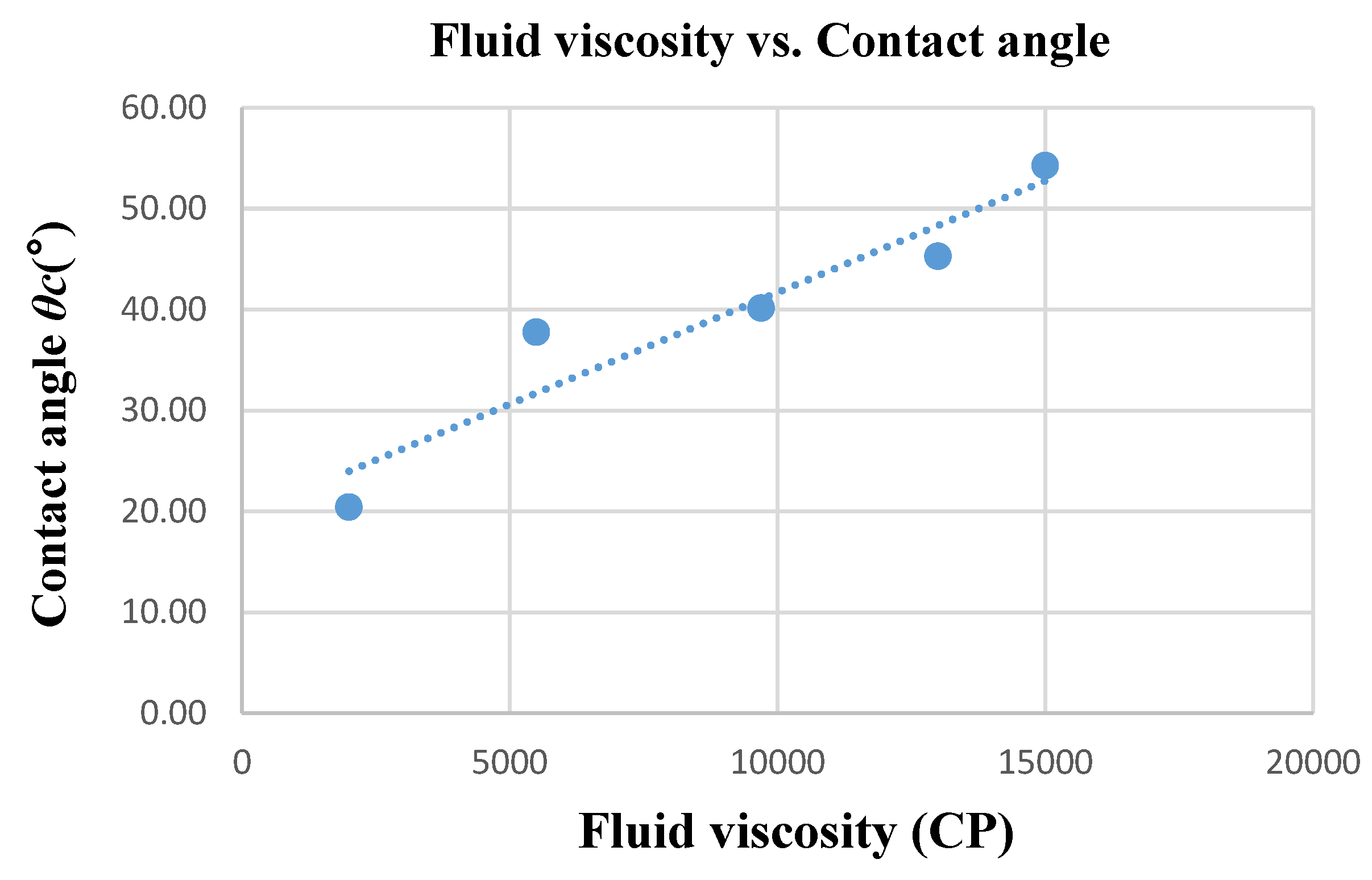
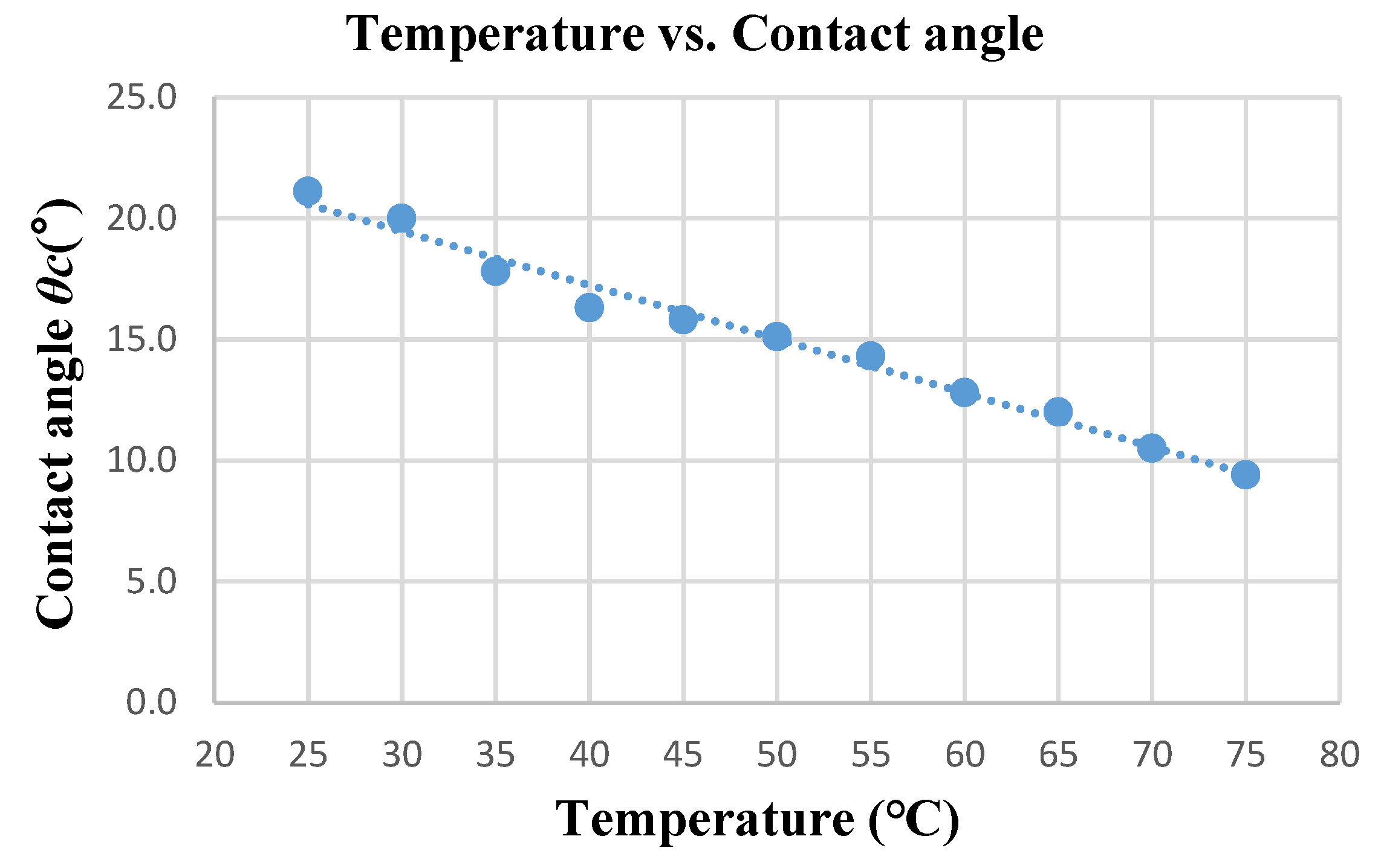
2.1. Surface Tension
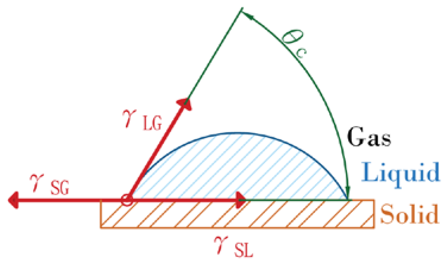
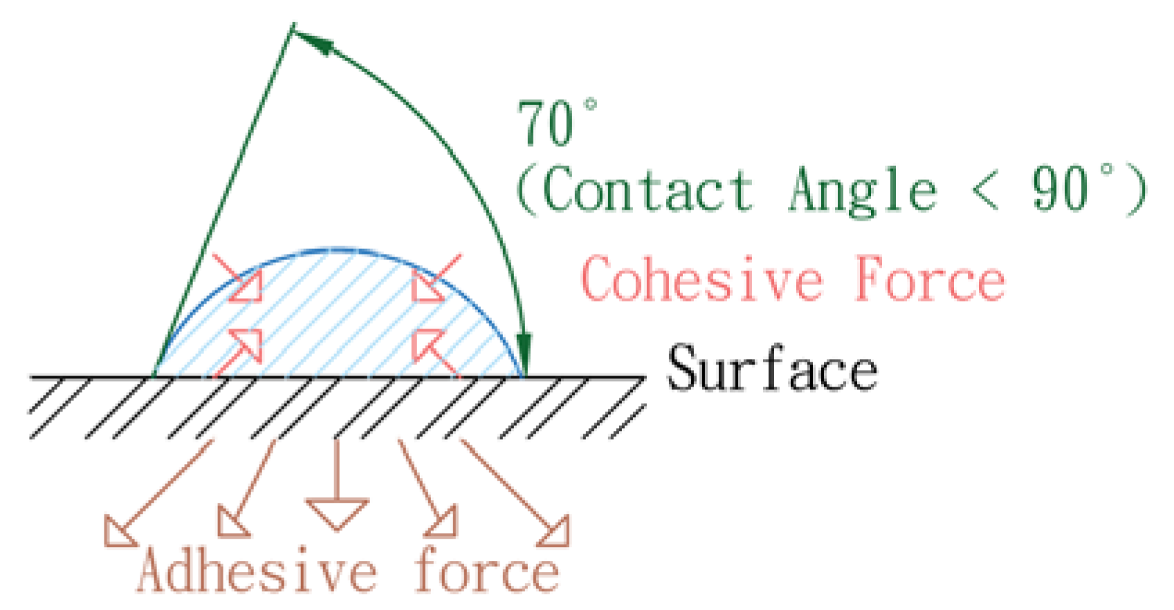
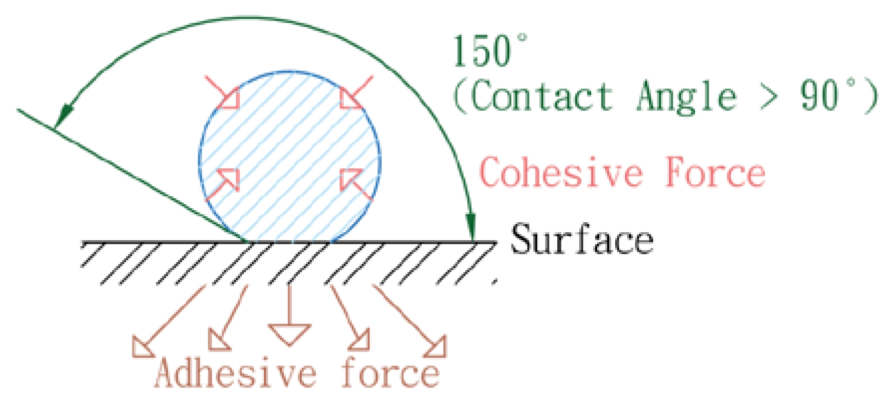
2.2. Contact Angle
2.3. Wettability
2.3.1. Degree of Wetness
2.3.2. Low Wettability
3. Equipment and Methods
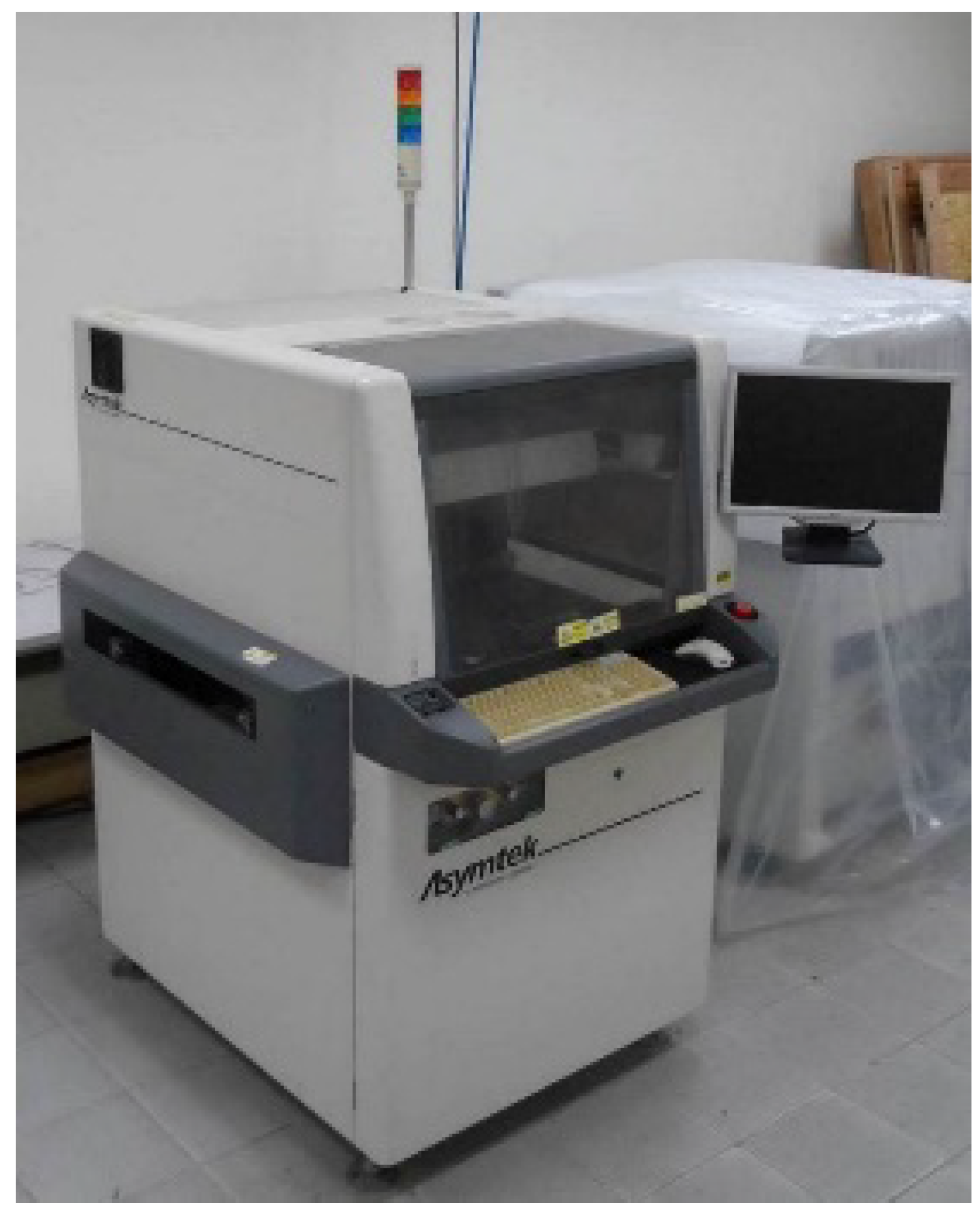
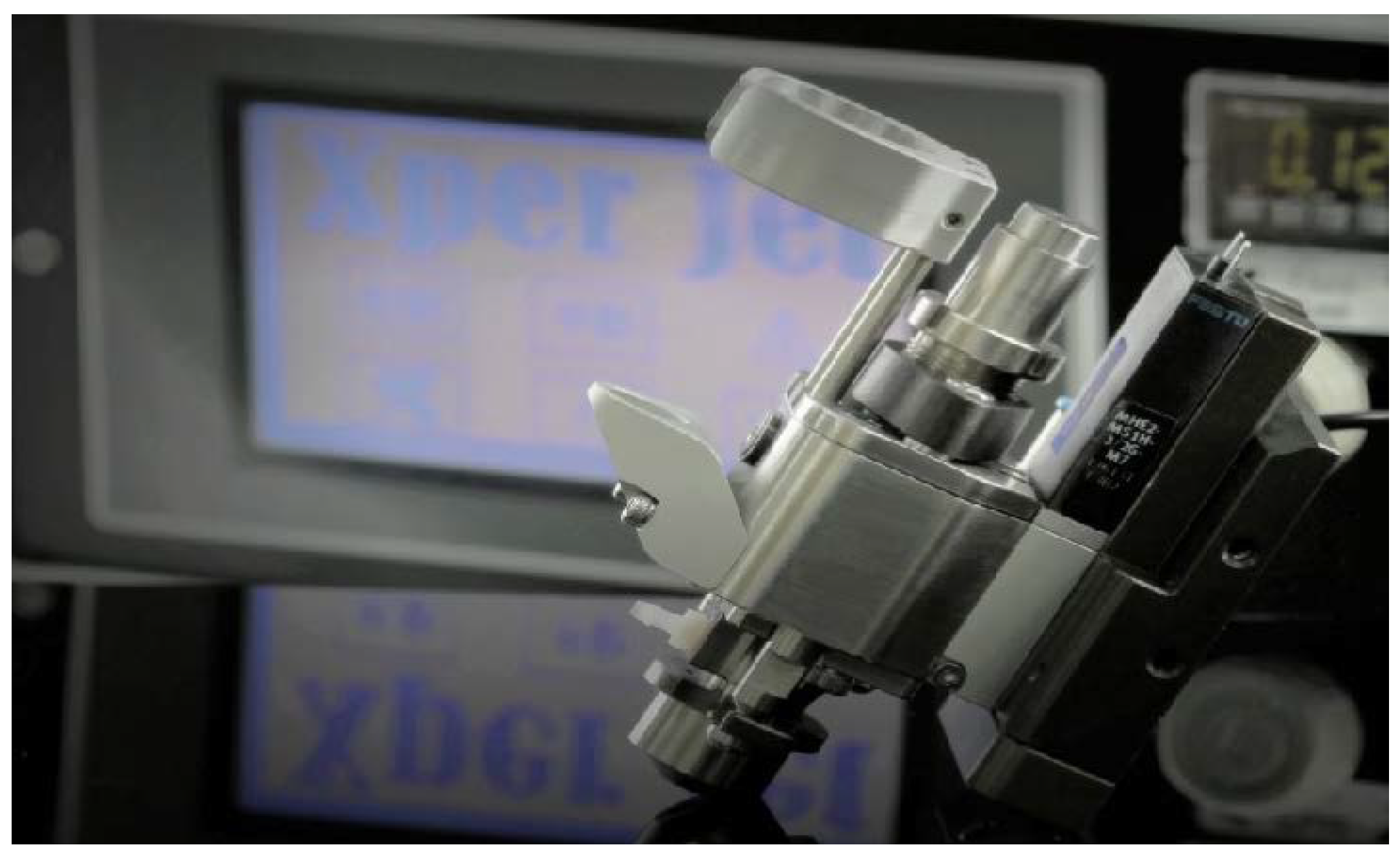
3.1. Dispensing System
3.2. Jet Valve
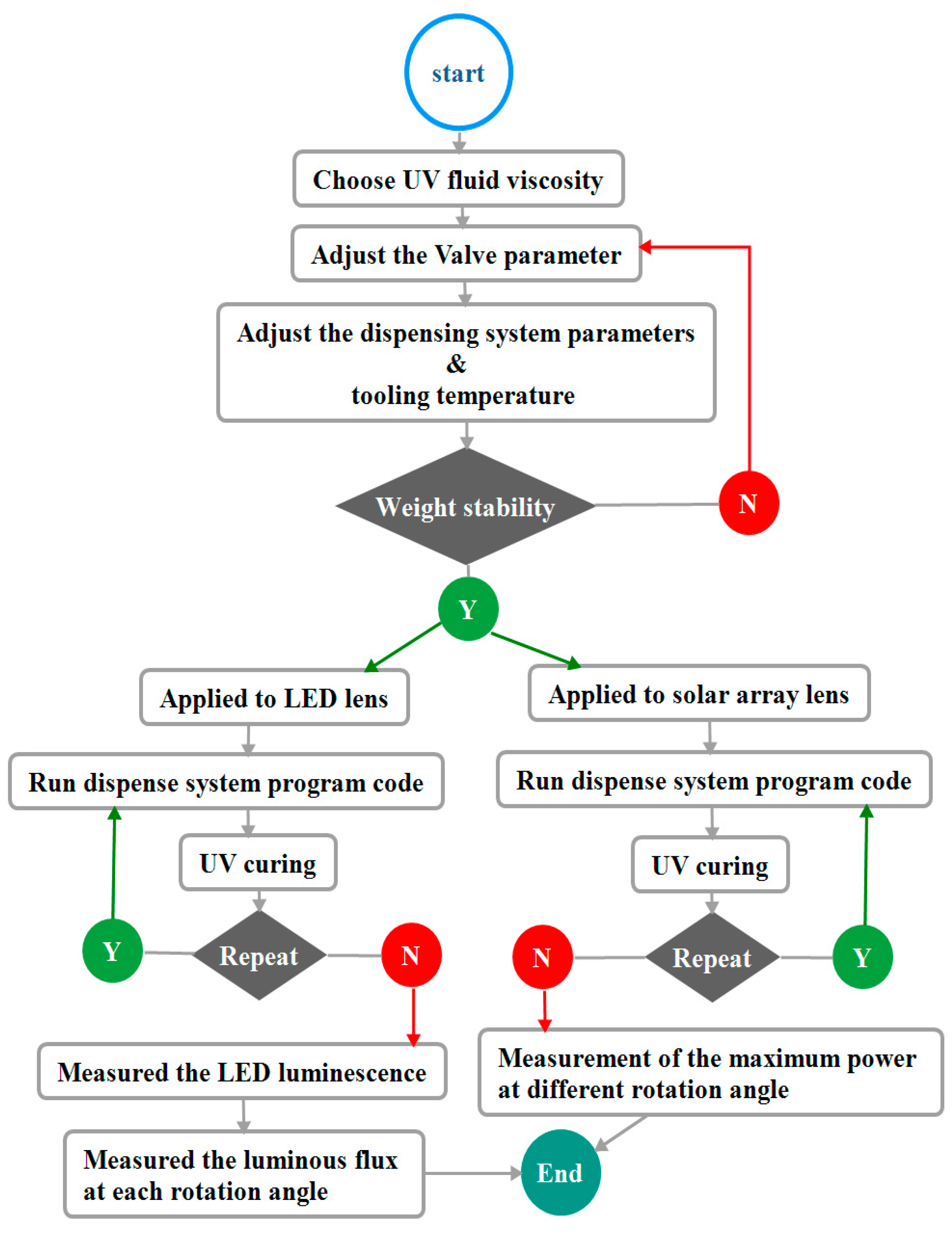
3.3. Description of Experimental Process
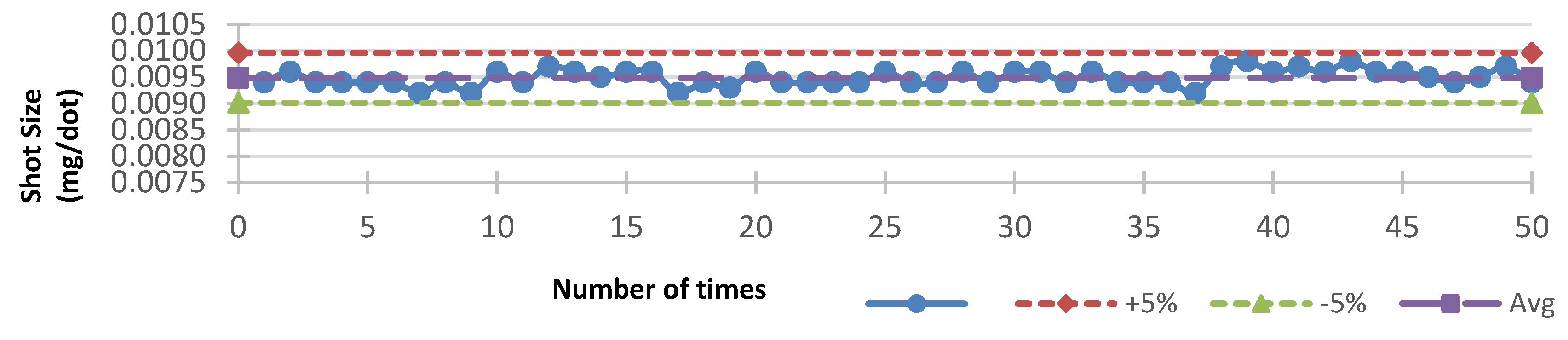
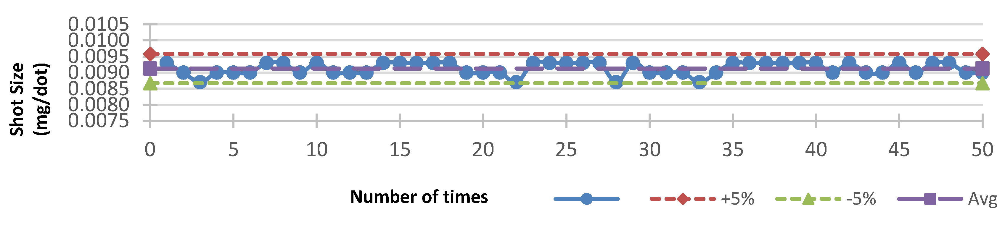
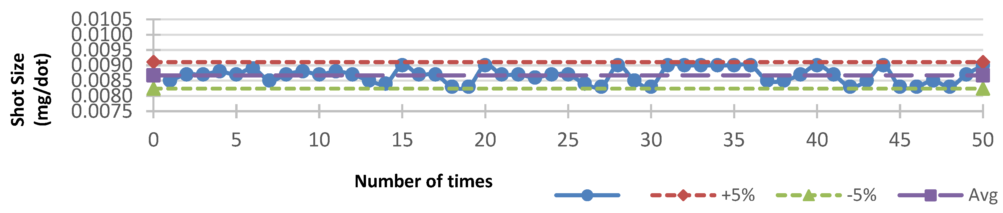
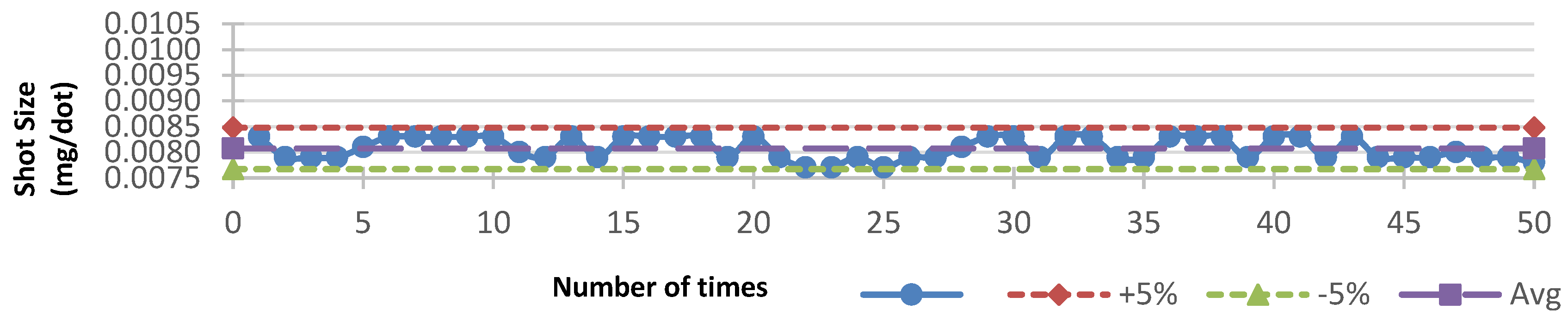
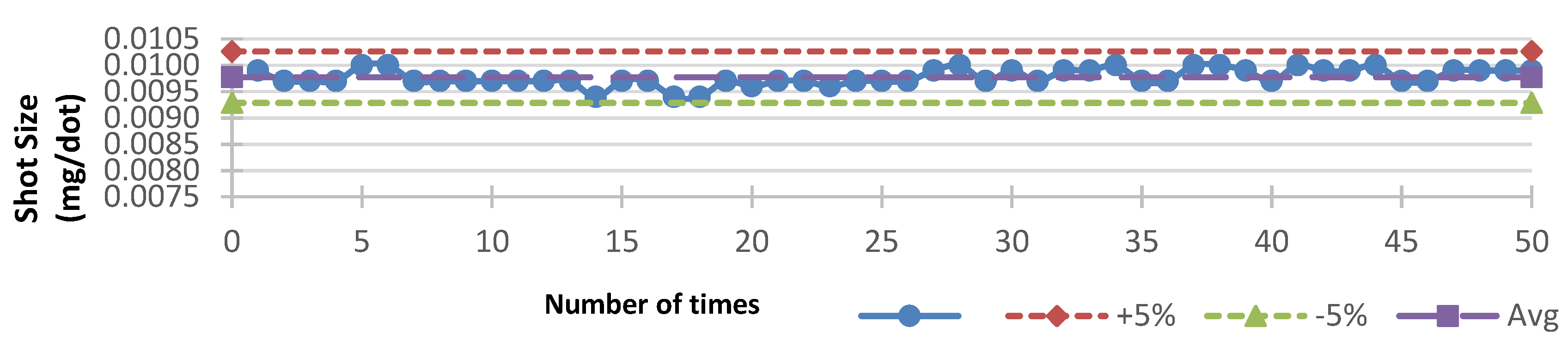
3.4. Weight Stability
4. Lens Production Experiment Results
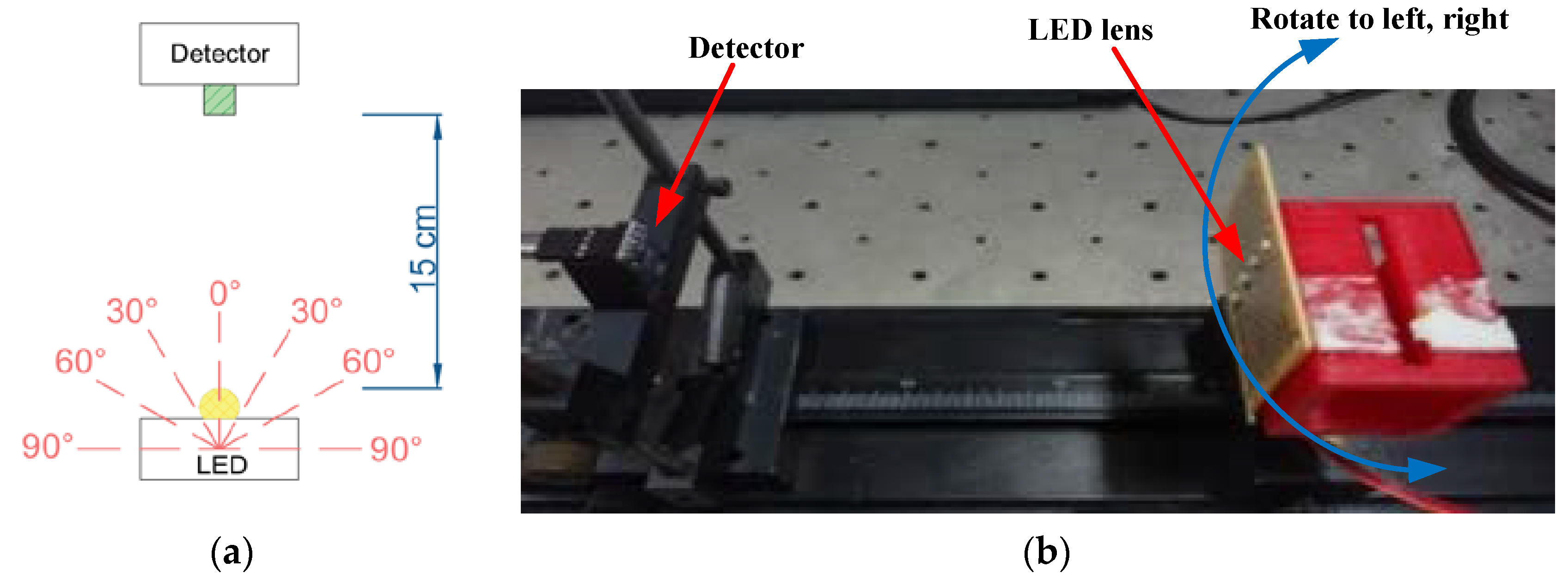
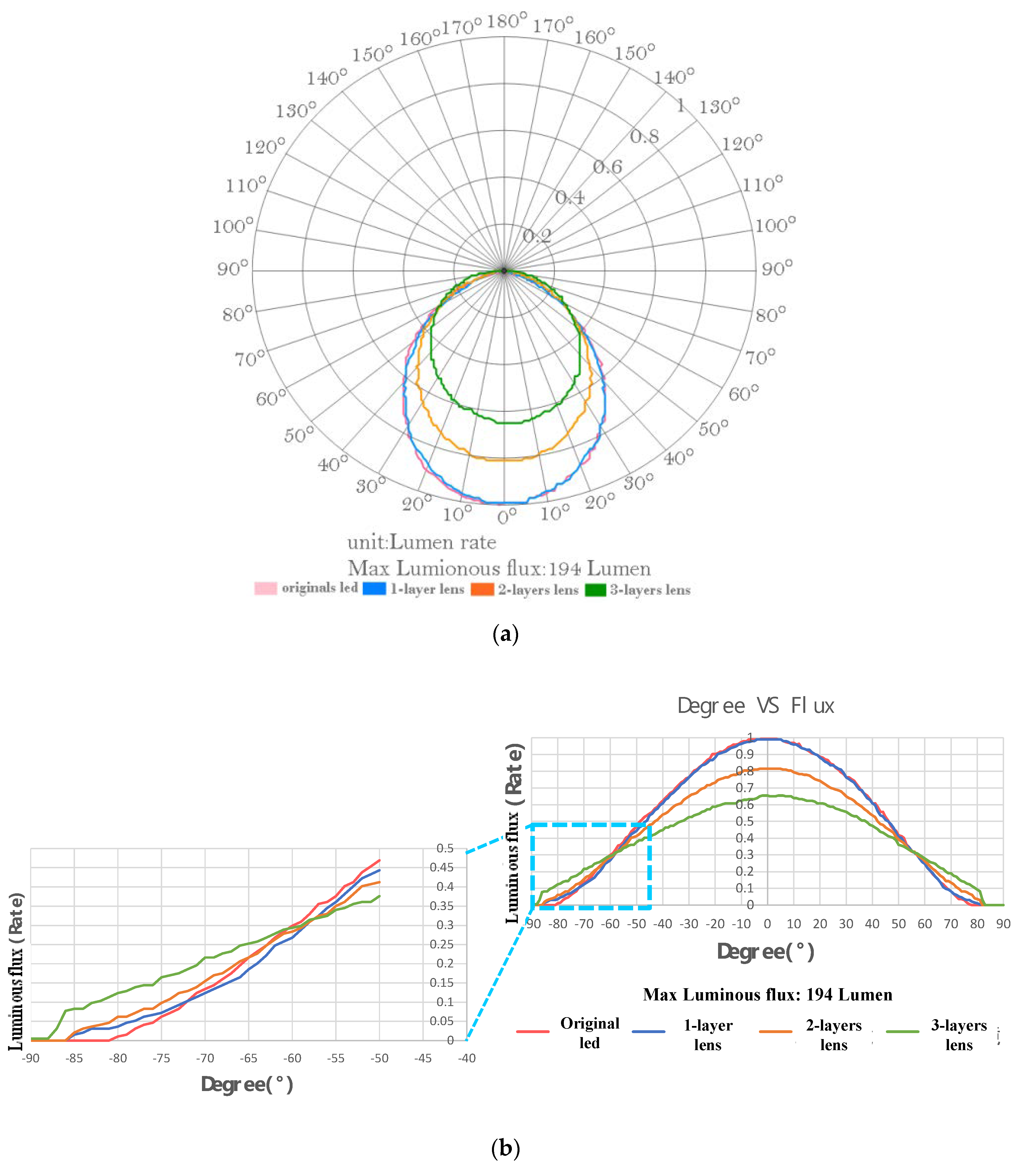
4.1. Applied to LED Lens
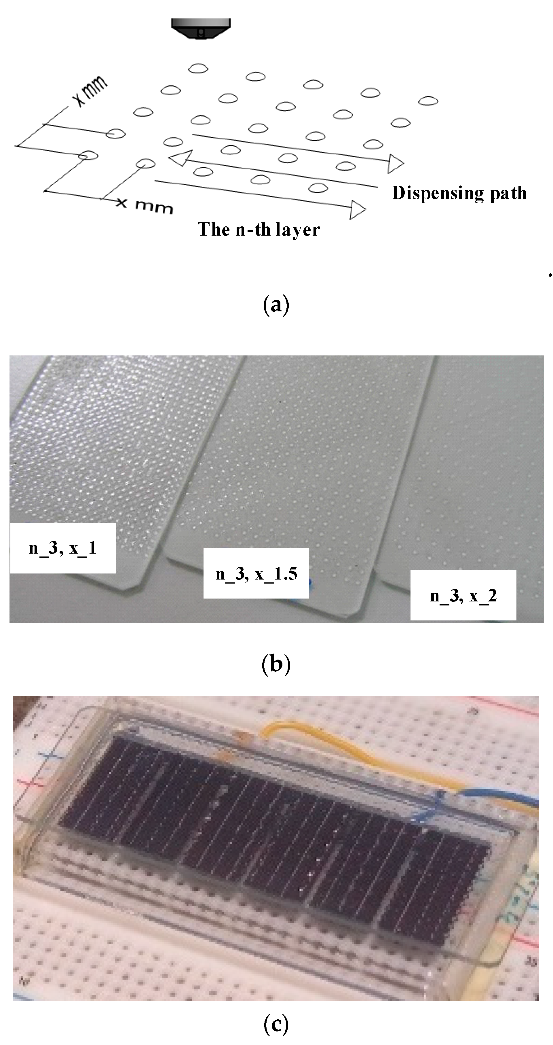
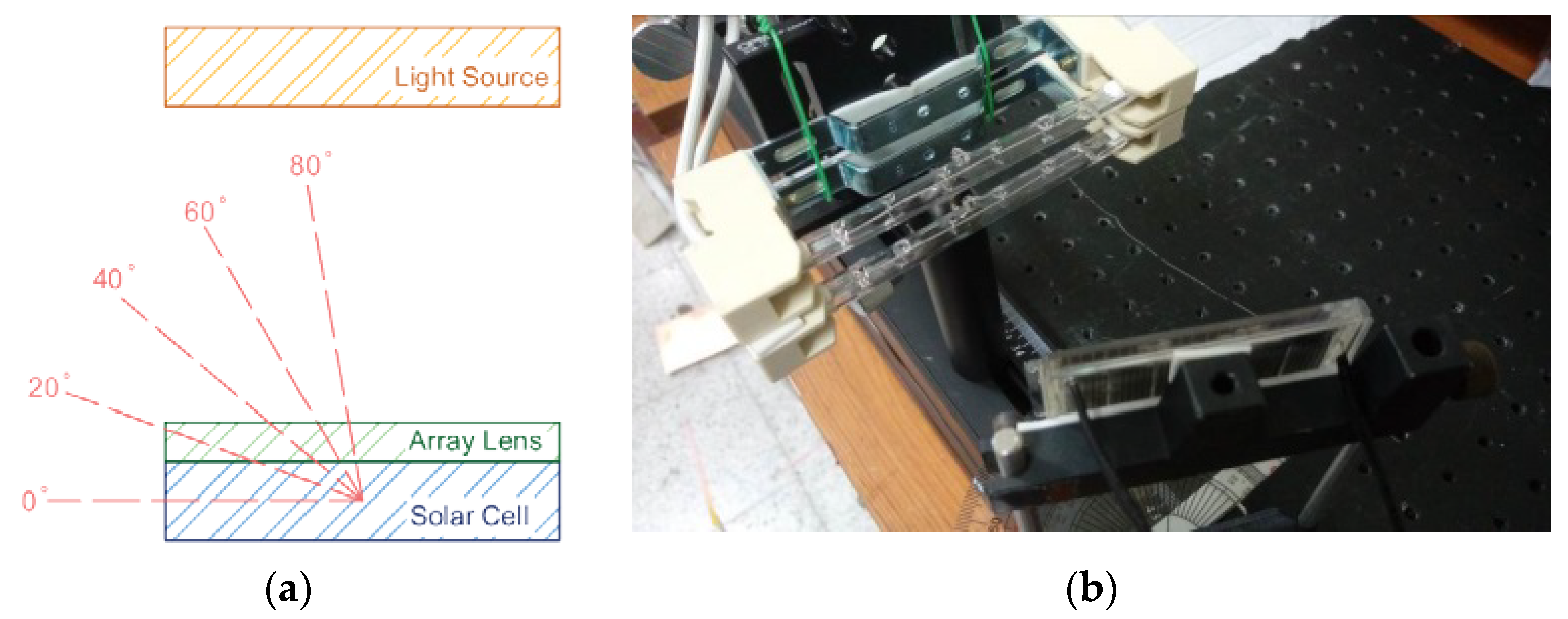
4.2. Lens Array Applied to Solar Cells
5. Conclusions
Author Contributions
Funding
Conflicts of Interest
References
- Furlan, W.D.; Ferrando, V.; Monsoriu, J.A.; Zagrajek, P.; Czerwinska, E.; Szustakowski, M. 3D printed diffractive terahertz lenses. Opt. Lett. 2016, 41, 1748–1751. [Google Scholar] [CrossRef] [PubMed]
- Zhang, S.; Arya, R.K.; Pandey, S.; Vardaxoglou, Y.; Whittow, W.; Mittra, R. 3D-printed planar graded index lenses. IET Microw. Antennas Propag. 2016, 13, 1411–1419. [Google Scholar] [CrossRef]
- MacFarlane, D.L.; Narayan, V.; Tatum, J.A.; Cox, W.R.; Chen, T.; Hayes, D.J. Microjet Fabrication of Microlens Arrays. IEEE Photonics Technol. Lett. 1994, 6, 1112–1114. [Google Scholar] [CrossRef]
- Luxexcel, 3D Printed Optics. Available online: https://www.luxexcel.com/ (accessed on 26 June 2017).
- McMahon, T.; Bonner, J.T. On Size and Life, Scientific; Holt & Company: Kosciusko, MS, USA, 1983. [Google Scholar]
- Young, T. An Essay on the Cohesion of Fluids. Philos. Trans. R. Soc. Lond. 1805, 95, 65–87. [Google Scholar] [CrossRef]
- Romi, S.; David, A.; Bruno, B.; Gorman, C.B.; Biebuyck, H.A.; Whitesides, G.M. Control of the Shape of Liquid Lenses on a Modified Gold Surface using an Applied Electrical Potential Across a Self-Assembled Monolayer. Langmuir 1995, 11, 2242–2246. [Google Scholar]
- Asymtek. Dispensing System Installation and Service Manual; Asymtek: Carlsbad, CA, USA, 2002; pp. 20–45. [Google Scholar]
- Asymtek. Fluidmove for Windows XP® Version 5.0 User Guide; Asymtek: Carlsbad, CA, USA, 2005; pp. 4–25. [Google Scholar]
- Mahajan, V.N. Fundamentals of Geometrical Optics; SPIE Press: Bellingham, WA, USA, 2014. [Google Scholar]

| Layers | 0 | 1 | 2 | 3 |
|---|---|---|---|---|
| CIE 1931_x | 0.321554 | 0.307743 | 0.302103 | 0.291521 |
| CIE 1931_y | 0.350373 | 0.318445 | 0.308519 | 0.291586 |
| CCT | 5966 | 6890 | 7407 | 8724 |
| CRI | 68 | 68 | 68 | 68 |
| LUX | 150 | 144 | 121 | 102 |
| Lens Shape | |||
|---|---|---|---|
 | 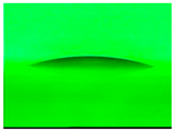 |  | |
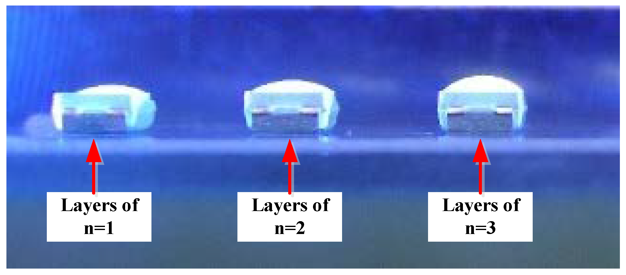
| Layers n | 3 | 10 | 15 |
| x (mm) | 2 | 2 | 2 |
| Lens height (μm) | 57.0 | 105.7 | 147.7 |
| Lens width (μm) | 936.7 | 1255.3 | 1457.3 |
| Contact angle θc (°) | 13.9 | 19.1 | 22.9 |
| n = 3 | |||
|---|---|---|---|
| x = 1 mm | x = 1.5 mm | x = 2 mm | |
| Top view | 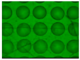 | 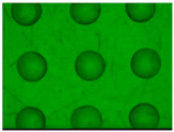 | 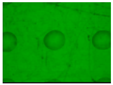 |
| Side view | 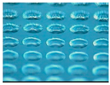 | 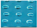 | 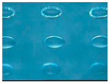 |
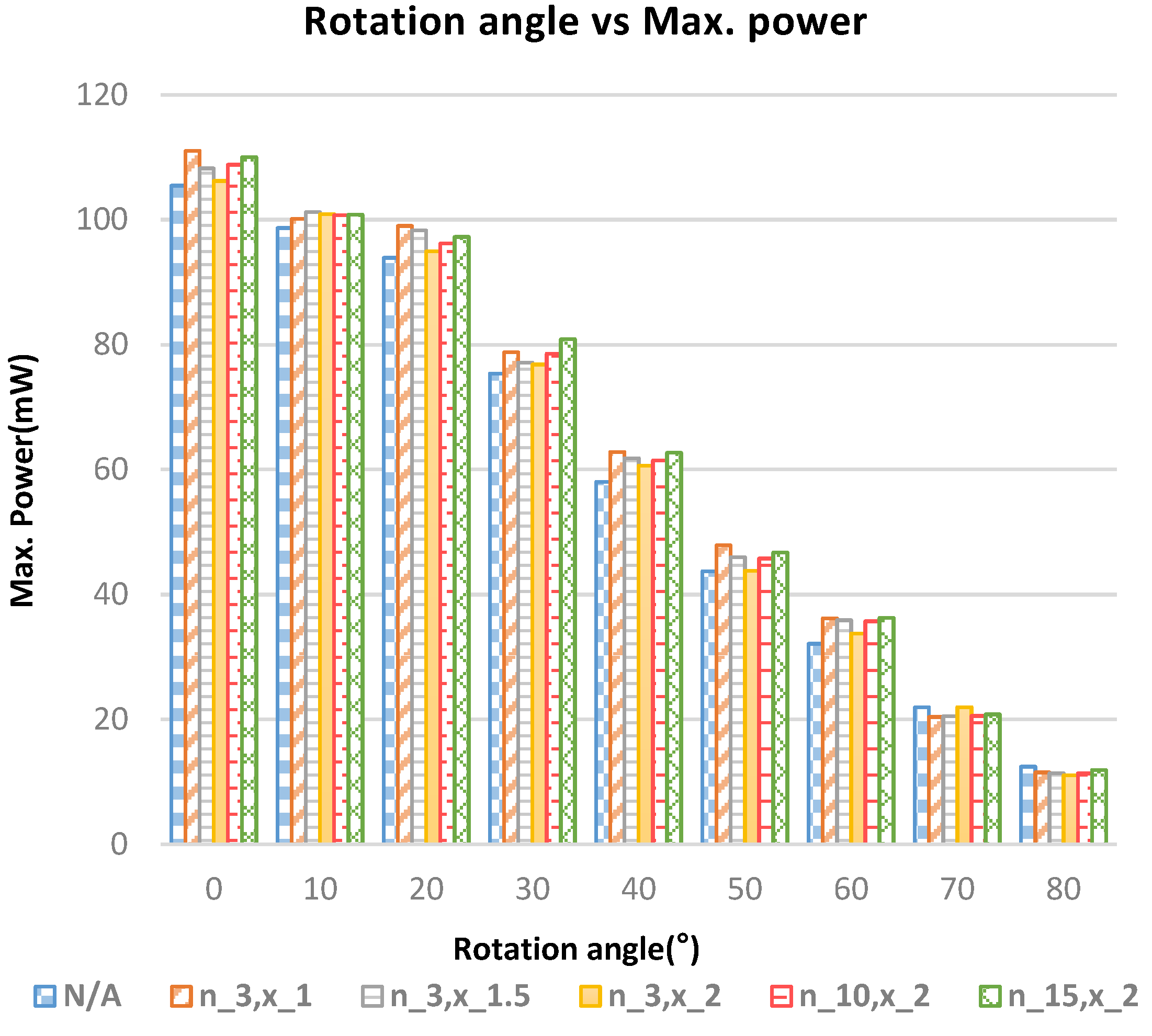
| Lens | N/A | n_3, x_1 | n_3, x_1.5 | n_3, x_2 | n_10, x_2 | n_15, x_2 |
|---|---|---|---|---|---|---|
| power generation (mW-hr) | 812.25 | 851.37 | 840.49 | 824.98 | 838.66 | 850.86 |
| Percentage of raise (%) | - | 4.82 | 3.48 | 1.57 | 3.25 | 4.75 |
© 2019 by the authors. Licensee MDPI, Basel, Switzerland. This article is an open access article distributed under the terms and conditions of the Creative Commons Attribution (CC BY) license (http://creativecommons.org/licenses/by/4.0/).
Share and Cite
Yu, F.-M.; Jwo, K.-W.; Chang, R.-S.; Tsai, C.-T. Dispensing Technology of 3D Printing Optical Lens with Its Applications. Energies 2019, 12, 3118. https://doi.org/10.3390/en12163118
Yu F-M, Jwo K-W, Chang R-S, Tsai C-T. Dispensing Technology of 3D Printing Optical Lens with Its Applications. Energies. 2019; 12(16):3118. https://doi.org/10.3390/en12163118
Chicago/Turabian StyleYu, Fang-Ming, Ko-Wen Jwo, Rong-Seng Chang, and Chiung-Tang Tsai. 2019. "Dispensing Technology of 3D Printing Optical Lens with Its Applications" Energies 12, no. 16: 3118. https://doi.org/10.3390/en12163118
APA StyleYu, F.-M., Jwo, K.-W., Chang, R.-S., & Tsai, C.-T. (2019). Dispensing Technology of 3D Printing Optical Lens with Its Applications. Energies, 12(16), 3118. https://doi.org/10.3390/en12163118