Spatial-Temporal Characteristics of the Driving Factors of Agricultural Carbon Emissions: Empirical Evidence from Fujian, China

Abstract

With the development of agricultural modernization, the carbon emissions caused by the agricultural sector have attracted academic and practitioners’ circles’ attention. This research selected the typical agricultural development province in China, Fujian, as the research object. Based on the carbon emission sources of five main aspects in agricultural production, this paper applied the latest carbon emission coefficients released by Intergovernmental Panel on Climate Change of the UN (IPCC) and World Resources Institute (WRI), then used the ordered weighted aggregation (OWA) operator to remeasure agricultural carbon emissions in Fujian from 2008–2017. The results showed that the amount of agricultural carbon emissions in Fujian was 5541.95 × 10³ tonnes by 2017, which means the average amount of agricultural carbon emissions in 2017 was 615.78 × 10³ tonnes, with a decrease of 13.13% compared with that in 2008. In terms of spatial distribution, agricultural carbon emissions in the eastern coastal areas were less than those in the inland regions. Among them, the highest agricultural carbon emissions were in Zhangzhou, Nanping, and Sanming, while the lowest were in Xiamen, Putian, and Ningde. In addition, this paper selected six influencing variables, the research and development intensity, the proportion of agricultural labor force, the added value of agriculture, the agricultural industrial structure, the per capita disposable income of rural residents, and per capita arable land area, to clarify further the impacts on agricultural carbon emissions. Finally, geographically- and temporally-weighted regression (GTWR) was used to measure the direction and degree of the influences of factors on agricultural carbon emission. The conclusion showed that the regression coefficients of each selected factor in cities were positive or negative, which indicated that the impacts on agricultural carbon emission had the characteristics of geospatial nonstationarity.

1. Introduction

Since the 21st Century, global warming, which is mainly caused by the increase of the carbon dioxide concentration in the atmosphere, has attracted widespread attention. Although the total carbon emissions are mainly from the industrial and service sectors, agricultural carbon emissions cannot be underestimated. The main reason for this is that although the agricultural sector provides food for all mankind, it also needs a large number of inputs of agricultural machinery and equipment, fertilizers, pesticides, agricultural film, and other means of production, which may ultimately lead to high carbon dioxide emissions. In addition, according to the statistics, the agriculture, forestry, and other land use sectors are responsible for about 24% of anthropogenic carbon emissions worldwide and have become the second largest source of global greenhouse gas emissions, and the emissions are also increasing at a fast speed of approximately 1% per annum [1,2]. Therefore, under the background of increasingly severe global warming, carbon emission reduction in the agricultural sector is an indispensable link to improve the capability of agriculture to cope with climate change and also an inevitable choice to achieve economic growth, ecological environmental development, and sustainable agricultural development. In other words, it is necessary to pay attention to the research on agricultural carbon emissions.

As a large traditional agricultural country in the world, China’s carbon emissions in the agricultural sector have a more noteworthy role in increasing global climate warming. Since 1978 and the progress of the reform and opening-up policy, China’s agriculture has developed rapidly and become an important factor to promote economic development and social progress. However, these rapid developments are largely at the expense of high carbon emissions. According to the statistics, the agricultural sector in China accounts for approximately 17% of national carbon emissions [3,4]. Among them, the emissions of methane and nitrogen dioxide caused by agriculture account for 50% and 92% of the national total, respectively. Thus, under the circumstances that China pledged to peak its carbon dioxide emissions by around 2030 and make best efforts to peak early, reducing carbon emissions in the agricultural sector has become a hot issue of academics and the government. In order to reduce carbon emission in the agricultural sector, first of all, it is necessary to clarify the carbon emission sources, carbon emission quantities, and influencing factors on carbon emissions. To this end, it is necessary to measure carbon emissions in the agricultural sector and identify the factors driving these carbon emissions.

As a coastal province in southeastern China, Fujian has some special features that are different from other provinces. Fujian has many mountains and few farmland, while the cultivated land resources are scarce, even less than half of the national average level, which seriously restricts the development of agriculture. Therefore, in order to promote the development of agricultural production, this can only be done by adding the inputs of chemical fertilizers, pesticides, and agricultural film for Fujian to increase the outputs of grain and other cash crops. However, these measures have resulted in a large amount of carbon emissions, causing serious environmental pollution. Besides, in 2014, Fujian became the first national ecological civilization pilot zone in China, which was announced by the State Council. That is, low-carbon agricultural development will become an important way to realize ecological civilization in Fujian Province, so as to realize finally the coordinated development of agriculture, resources, and the environment. Hence, in order to effectively promote the reduction of carbon emissions in the agricultural sector and complete the construction of the ecological civilization pilot zone, it is of great significance to carry out research on Fujian’s agricultural carbon emissions. Thus, this research takes the prefecture-level cities as the basic units to analyze the spatial and temporal pattern and the evolution process of agricultural carbon emissions in Fujian and then explores the influencing factors affecting agricultural carbon emissions, so as to provide scientific evidence for formulating agricultural carbon emission reduction policies and realizing low-carbon agriculture in Fujian.

Compared with the existing research, the innovative work of this research is mainly manifested in the following three aspects. Firstly, the study area of this paper is specific. More concretely, although some scholars’ research involves the issue of agricultural carbon emissions, most of them stay at the macro level, that is the literature specific to a certain area is less [5]. Therefore, based on the data of nine prefecture-level cities in Fujian, this research remeasured the agricultural carbon emissions by using the latest emission coefficients released by the Intergovernmental Panel on Climate Change of UN (IPCC, Geneva, Switzerland) and World Resources Institute (WRI, Washington, DC, USA), so as to achieve more accurate calculation of carbon emissions in the agricultural sector. Secondly, a more scientific method was used to evaluate the agricultural carbon emissions of each prefecture-level city in the sample period. Different from other existing research using the simple arithmetic averaging method, this paper uses the ordered weighted averaging (OWA) aggregation operator to distribute weights in different years, so as to solve the problem of weighting the same indicators in different periods ignored in the calculation of carbon emissions, so as to realize the dynamic comprehensive evaluation of panel data. Moreover, agricultural carbon emissions are mainly the result of multivariate interaction, such as economic level, the infrastructure, and resource endowment. The mechanism of the above action is complex. Therefore, the magnitude and direction of the influencing factors are different under different in their temporal and spatial distributions. That is, traditional spatial econometric models will no longer meet the research requirements. The geographically- and temporally-weighted regression (GTWR) applied in this research is a local linear regression model that considers both geographical and temporal non-stationarity. On the whole, this study measures carbon emissions in the agricultural sector and uses the OWA aggregation operator to solve the problem of the dynamic comprehensive evaluation of panel data. Then, by adopting the GTWR model, this paper analyzes the spatial-temporal heterogeneity of the impact of factors on agricultural carbon emissions, aiming to establish an effective agricultural carbon emission reduction mechanism, and finally, aiding local sustainable development decision-making.

2. Literature Review

2.1. Measurement of Agricultural Carbon Emissions

At present, many existing research works have focused on the measurement of carbon emissions in the agricultural sector. It should be noted that different methods used to estimate carbon emissions will produce different results. For instance, Wang et al. followed the IPCC guidelines [6] released in 2006 to estimate the greenhouse gas emission intensity of rice, wheat, and maize yields in China from 1985–2010 [7]. According to the IPCC guidelines, Xiong et al. and Tian et al. estimated the carbon emissions of agricultural production in Hunan and Xinjiang, respectively [8,9]. In addition, Han et al. measured carbon emissions from the entire agricultural sector as a whole in China during the period from 1997–2015 [10]. However, the IPCC guidelines ignored soil emissions during agricultural land use change in its agricultural inventory [11,12] and are no longer fully suitable for current emissions. Therefore, some scholars have proposed novel methods to measure agricultural carbon emissions. For instance, Bell et al. used the Scottish Government’s new method to calculate agricultural carbon emissions and compared it with the IPCC guidelines and national communications [12]. Wisniewski and Kistowski proposed a solution that enables local governments to estimate independently the carbon footprints and monitor the impacts of actions taken to reduce emissions [13]. Moreover, based on the national statistics, Yue et al. evaluated the carbon footprints of a range of 26 crop products and six livestock types [14]. Based on the above background, this paper applied the carbon emission coefficients released by IPCC and WRI to calculate the agricultural carbon emissions in Fujian from 2008–2017, which makes the measurement results more specific and accurate.

2.2. Influencing Factors of Agricultural Carbon Emissions

The driving and inhibiting factors of agricultural carbon emissions can be identified by studying the influencing factors of agricultural carbon emissions. Existing research on the influencing factors of agricultural carbon emissions mainly involves many aspects, including agricultural economic growth, technological progress, population size, income, and agricultural energy consumption. ACIL Tasman measured agricultural carbon emissions in the United States, Canada, India, the European Union, and New Zealand and demonstrated that the proportion of agricultural carbon emissions in total carbon emissions varies greatly, possibly due to different modes of agricultural production [5]. Ismael et al. also confirmed that agricultural production had a significant impact on carbon emissions [15]. For instance, the organic agricultural production mode had the function of restraining agricultural carbon emissions [16]. In addition, agricultural economic growth and the increase of the agricultural population has positive impacts on agricultural carbon emissions [11,17]. Moreover, the agricultural technology progress is also one of the important factors affecting agricultural carbon emissions. Gerlagh applied the endogenous technological progress model to study the influence of technological progress on carbon emission reduction [18] and confirmed that technological progress significantly reduced the cost of carbon emission reduction through the learning effect and increased the social benefits at the same time. Furthermore, agricultural land also affects the agricultural carbon emissions, such as per capita land use area [19], agricultural land use [20] and farmland conversion [21,22]. Besides, there also exists a close relationship between agricultural income and carbon emissions [23].

However, it should be noted that there is still no consensus on the causal relationship, direction, and extent between influencing factors and agricultural carbon emissions. Hence, when selecting the influencing factors, we should combine the relevant literature with the outstanding characteristics of Fujian in the process of agricultural development, so as to ensure that the factors are reasonable and scientific.

2.3. Methodologies of Agricultural Carbon Emissions

There exist many methodologies to explore the relationship between carbon emissions and their influencing factors in the agricultural sector. Among them, the autoregressive distribution lag model [24], the Granger causality test [25,26], and the vector error correction model [27] have been approved and applied by most scholars. Moreover, the logarithmic mean Divisia index [28,29] and the variance decomposition approach [15] mainly apply the exponential decomposition method to study the main factors causing the change of agricultural carbon emissions. Furthermore, other scholars have applied some other novel methodologies, including the denitrification-decomposition models [30], the spatial econometric models [25] and the fully-modified ordinary least squares [31,32].

However, when examining the degree and direction of the impact factors on agricultural carbon emissions, most of the literature only considers the time perspective, but ignores the spatial perspective. It should be noted that there exist great differences in the level of economic development, agricultural structure, resource endowment, and the agricultural production mode in each region, which will also lead to different degrees and directions of influencing factors at different times and in different regions. Hence, in this paper, the GTWR model is used to study the influences of factors affecting agricultural carbon emissions on each prefecture-level city from the perspective of time and space, so as to remedy the shortcomings of this research field.

3. Materials and Methodologies

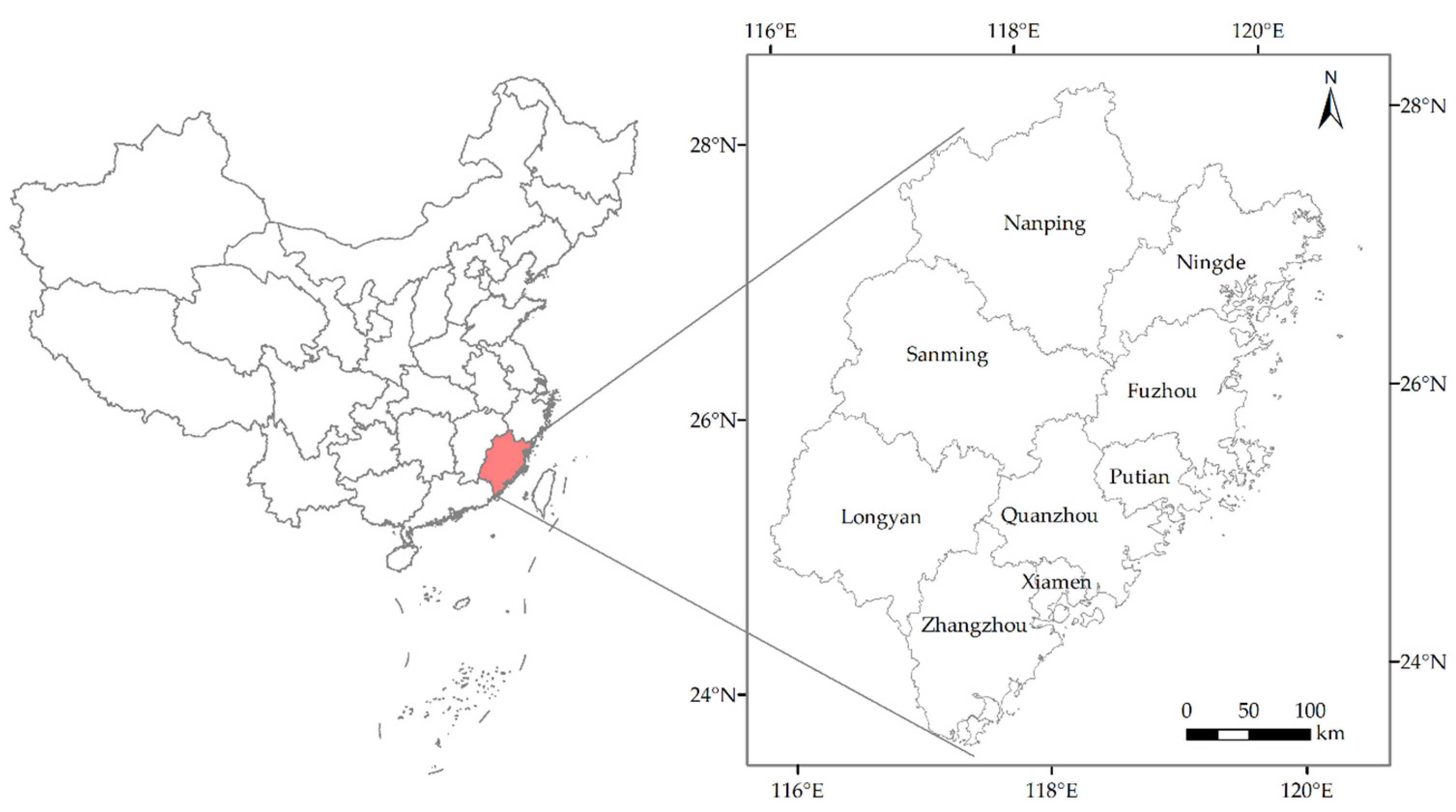
3.1. Study Area

The study area covers Fujian on the southeast coast of China. As an important estuary for the Min River and also an important window for China’s contacts with the world, Fujian encompasses a total land area of approximately 124,000 km² and a total maritime area of approximately 136,000 km². From the geographical perspective, Fujian is located approximately between longitudes 115°50′ E and 120°43′ E and between the latitudes 23°32′ N and 28°22′ N. As one of the provincial administrative regions in China, Fujian includes 9 prefectural-level cities: Fuzhou, Xiamen, Quanzhou, Zhangzhou, Sanming, Putian, Longyan, Nanping, and Ningde. According to the Fujian Statistical Yearbook, from 2010–2018, the gross output value of agriculture in Fujian increased from 136.367–237.982 billion Yuan at a rapid rate. Similarly, per capita disposable income of rural residents increased from 7426.86–17,821 Yuan. However, the rapid development of agriculture is at the expense of the environment. That is, at present, the agricultural development in Fujian is a typical chemical agriculture type, which relies heavily on high-carbon means of production such as chemical fertilizers and pesticides, which seriously affects the sustainable development of agriculture in the future. Thus, it is of great practical significance to study agricultural carbon emissions and their influencing factors in Fujian and to explore the way to realize the development of low-carbon agriculture. The location, the latitude and the longitude rage of the study area can be seen in Figure 1.

3.2. Selection of Measurement Indicators

In agriculture, there exist three main sources of carbon emissions, which can also be considered as sources of greenhouse gas emissions: agricultural land use, rice paddies and crop production, and livestock enteric fermentation and manure storage. In the United States, agricultural land use is the largest source of agricultural carbon emissions, mainly due to the large inputs of fertilizers, pesticides, and other agricultural materials and the loss of organic carbon caused by soil tillage; livestock enteric fermentation is the second largest source, and livestock manure storage is the third. Furthermore, the rice paddies produce fewer greenhouse gases than other agricultural productions because of the lesser rice planting area. Although Fujian’s agricultural production situation differs from that of the United States, the composition of agricultural carbon emissions is consistent. Therefore, combining the above research with other references [17,23], this paper mainly calculates the agricultural carbon emissions according to the five types of carbon emission sources: (1) CO₂ emissions produced from agricultural land use; (2) CH₄ emissions caused by rice paddies; (3) CH₄ emissions caused by livestock breeding; (4) N₂O emissions triggered by crop production; (5) N₂O emissions triggered by livestock breeding. All carbon emission sources and their coefficients in agricultural sector in Fujian are listed in

Table 1. Carbon emission sources and coefficients in the agricultural sector.

Sources	Detailed Sources	Units	Greenhouse Gases			References
			CO2	CH4	N2O
agricultural land use	chemical fertilizer	kg/kg	3.28	n/a	n/a	IPCC
	pesticide	kg/kg	18.09	n/a	n/a	IPCC
	plastic sheeting	kg/kg	19.00	n/a	n/a	IPCC
	diesel	kg/kg	3.17	n/a	n/a	IPCC
	tillage	kg/km2	1146.31	n/a	n/a	IPCC
	irrigation	kg/ha	977.19	n/a	n/a	IPCC
rice paddies	early rice	kg/ha	n/a	77.39	n/a	IPCC
	late rice	kg/ha	n/a	525.95	n/a	IPCC
	in-season rice	kg/ha	n/a	434.66	n/a	IPCC
crop production	paddy rice	kg/ha	n/a	n/a	0.24	IPCC
	winter wheat	kg/ha	n/a	n/a	2.05	IPCC
	soybean	kg/ha	n/a	n/a	0.77	IPCC
	vegetable	kg/ha	n/a	n/a	4.21	IPCC
	maize	kg/ha	n/a	n/a	2.53	IPCC
	other dry crops	kg/ha	n/a	n/a	0.95	IPCC
livestock: manure storage	dairy	kg/head/year	n/a	8.33	2.07	WRI
	non-dairy	kg/head/year	n/a	3.31	0.85	WRI
	goat	kg/head/year	n/a	0.28	0.11	WRI
	pig	kg/head/year	n/a	5.08	0.18	WRI
	poultry	kg/head/year	n/a	0.02	0.01	WRI
	rabbit	kg/head/year	n/a	0.08	0.02	IPCC
livestock: enteric fermentation	dairy	kg/head/year	n/a	89.3	n/a	WRI
	non-dairy	kg/head/year	n/a	67.9	n/a	WRI
	goat	kg/head/year	n/a	9.4	n/a	WRI
	pig	kg/head/year	n/a	1	n/a	WRI
	poultry	kg/head/year	n/a	n/a	n/a	WRI
	rabbit	kg/head/year	n/a	0.25	n/a	IPCC

Note: Data of IPCC and WRI in the column of the “References” are from [6] and [33], respectively.

.

3.3. Selection of Influencing Factors

3.3.1. Research and Development Intensity

Agricultural technological progress is an important factor to promote the development of low-carbon agriculture and has the role of agricultural carbon emission reduction [34]. Hence, the absence of agricultural technology has become an important factor restricting the sustainable development of agriculture [35]. Therefore, it is necessary and effective for governments to increase the input intensity of research and development and promote the progress of agricultural technology to further improve the technical system of energy saving and emission reduction in agriculture [10,36]. It is noteworthy that the current role of science and technology input is not necessarily reflected in the current period, such as R & D investment [37]. R & D investment will take effect only after a later period of time. Thus, it is necessary to consider the lagged rank of R & D investment affecting agricultural carbon emissions in a certain period of time. The proportion of R & D investment to GDP is adopted in this research to measure the science and technology intensity and denoted as research and development intensity (RDI).

3.3.2. Proportion of Agricultural Labor Force

Agricultural labor force (ALF) can affect the carbon emissions from crop production [9], which in turn affects agricultural carbon emissions. Based on the Kaya model, Zhang and Fang decomposed factors affecting agricultural carbon emissions and found that reducing the proportion of agricultural labor can significantly limit the growth of carbon emissions [38]. According to the logarithmic mean Divisia index (LMDI) method, Yao et al. confirmed that the increase of agricultural labor force is an important factor for the sustained growth of carbon emissions produced from animal husbandry [39]. Similarly, Satterthwaite [40] and Al-Mulali et al. [41] analyzed the relationship between agricultural labor force and agricultural carbon emissions from the perspective of urbanization and confirmed that with the acceleration of urbanization, the proportion of agricultural labor force continued to decline and then had a positive impact on the reduction of carbon emissions. The proportion of agricultural labor force in Fujian decreased from 31.15–21.71% during the time period from 2008–2017, which inevitably had an influence on agricultural carbon emissions.

3.3.3. Added Value of Agriculture

This paper applies the proportion of added value of agriculture (AVA), forestry, animal husbandry, and fishery production to measure the level of agricultural economic development. By and large, the influence of agricultural added value on agricultural carbon emissions has regional characteristics. Tian et al. combined multiple linear regression with decoupling analysis to evaluate the influencing factors of agricultural carbon emission and found that there was a weak and unstable decoupling relationship between agricultural carbon emissions and the added value [9]. Murad also confirmed that there existed no Granger causality between agricultural output and carbon emissions in Bangladesh [42]. However, Jebli et al. [43] and Rafiq [44] confirmed that there was a two-way causal relationship between agricultural added value and carbon dioxide emissions. Besides, by using data from provinces from 2001–2013 in Iran, Alamdarlo demonstrated that there existed an inverted “U” relationship between agricultural value added and agricultural carbon emissions; however, the above conclusion was not suitable for all provinces, because of the heterogeneity of agricultural development in provinces, such as the disunity of agricultural infrastructure [45]. Hence, it is necessary to analyze the impact of the influencing factor based on the specific situation of agricultural development in Fujian.

3.3.4. Agricultural Industrial Structure

The percentage of the output value of the plant products industry to total agricultural output value is applied in this paper to measure the structure of agricultural industry. The plant products industry mainly relies on the input of agricultural materials such as pesticides and fertilizers to increase output, resulting in an increase in agricultural carbon emissions. Hence, with the optimization of the agricultural industrial structure (AIS), the decline of the proportion of plant products industry can reduce agricultural carbon emissions [29]. Nevertheless, Yao et al. obtained slightly different conclusions by studying the influencing factors of the agricultural carbon emission change in animal husbandry [39]. They found that the impact of the optimization of agricultural industrial structure on carbon emissions from animal husbandry changed from positive to negative, which is particularly evident in central and Eastern China. Therefore, empirical research is needed to analyze the direction and magnitude of the impacts of agricultural industrial structure on agricultural carbon emissions in Fujian.

3.3.5. Per Capita Disposable Income of Rural Residents

In 1993, Panayotou first introduced and named the relationship between economic growth and environmental conditions as the environmental Kuznets curve (EKC), indicating that per capita income had a strong inverted “U” curve relationship with the level of environmental pollution [46]. However, Liu and Xin confirmed that the evolutionary trend between economic growth and agricultural carbon emissions showed an “N” curve, indicating that agricultural carbon pollution becomes more serious than before as the economy continues to expand [47]. In addition, Tian et al. also demonstrated that when per capita income of agriculture increased by 1 unit, agricultural carbon emissions would increase by 0.354 units [9]. One explanation could be that while vigorously increasing the per capita income of agriculture, the extensive use of chemical fertilizers and pesticides into agriculture promoted the increase of carbon emissions [48]. Therefore, the increase of rural residents’ income at this stage may lead to an increase in agricultural carbon emissions.

3.3.6. Per Capita Arable Land Area

Reducing per capita arable land area (ALA) will reduce the total agricultural energy demand per capita, such as chemical fertilizers, pesticides, and plastic film, thus restraining agricultural carbon emissions [19]. However, if the per capita arable land area were reduced through the transformation of cultivated land to industrial land, the greenhouse effect would be aggravated [49]. Thus, the degraded land can be restored by returning cultivated land to grassland. That is, reducing arable land area is conducive to reducing greenhouse gas emissions from agricultural activities. In brief, the land use and land use change in the agricultural sector are two important factors influencing agricultural carbon emissions [50].

3.4. Research Methodologies and Data Sources

3.4.1. Estimation of Agricultural Carbon Emissions

According to the IPCC guidelines, on the basis of the existing research about the carbon emission equation [20,28,29,36], in view of the current situation of agricultural development in Fujian Province, this paper chooses carbon emission sources and corresponding carbon emission coefficients to build a model for calculating agricultural carbon emissions. The specific formula is as follows:

$$E={\displaystyle \sum _{i=1}^n{E}_i}={\displaystyle \sum _{i=1}^n{T}_i·{\mu }_i}$$

(1)

where E represents total agricultural carbon emissions; E_i denotes the carbon emission of the specific source i; T_i represents the amount of the specific source i; and μ_i denotes carbon emission coefficient of the specific source i. In accordance with the usual practice, it is necessary to convert CO₂, CH₄, and N₂O to standard carbon. By and large, the greenhouse effects caused by 1 tonne of CO₂, CH₄, and N₂O are equivalent to that produced by 0.2727, 6.8182, and 81.2727 tonnes of standard carbon, respectively.

3.4.2. Ordered Weighted Averaging Aggregation Operator

The ordered weighted averaging (OWA) aggregation operator, first proposed by Yager in 1988, is a novel time empowerment method. The basic idea of OWA is to reorder the data according to the numerical value and then determine the weight by the position of the data in the ranking [51]. In addition, the OWA aggregation operator determines the weights based on the data themselves; therefore, since it was introduced into the application, the fairness of its empowerment has been controversial. Scholars in various countries have constantly improved it. Hence, in this paper, an improved OWA aggregation operator proposed by Xu [52], that is a smooth and continuous normal distribution density function, is applied to determine the time weights of the panel data of agricultural carbon emissions in Fujian. The specific steps of the OWA aggregation operator are as follows:

(1) Assume that there exist m regions and n years; besides, E_ij denotes total carbon emissions in the agricultural sector in specific region i in specific year j. After summing up the value of E_ij in each year, the average value is as follows:

$${\overline{E}}_j=\frac{1}{m}{\displaystyle \sum _{i=1}^m{E}_{ij}}$$

(2)

(2) Assume that the initial weights of total carbon emissions in each year is 1/n, then the average value and standard deviation of E_ij are as follows:

$$\overline{E}=\frac{1}{n}{\displaystyle \sum _{j=1}^n{\overline{E}}_j}$$

(3)

$$\sigma =\sqrt{\frac{{\displaystyle \sum _{j=1}^n{({\overline{E}}_j-\overline{E})}^2}}{n}}$$

(4)

(3) Standardize the total carbon emissions based on the above average value and standard deviation, and the calculation equation is as follows:

$${\beta }_j=\frac{{\overline{E}}_j-\overline{E}}{\sigma }$$

(5)

(4) Using the standard normal distribution density function, the corresponding values of α_j under the specific β_j are as follows:

$${\alpha }_j=\phi ({\beta }_j)=\frac{1}{\sqrt{2\pi }}{e}^{-\frac{{\beta }_j^2}{2}}$$

(6)

(5) Normalize the obtained value of α_j to calculate the time weights, and the formula is as follows:

$${\omega }_j=\frac{{\alpha }_j}{{\displaystyle \sum _{j=1}^n{\alpha }_j}}$$

(7)

3.4.3. Geographically- and Temporally-Weighted Regression

When exploring the relationship between agricultural carbon emissions and influencing factors in the past, the ordinary least squares method and the spatial econometric model were usually used. Normal panel models usually only represent the correlation between dependent and independent variables in the mean sense, but cannot effectively reflect the spatial heterogeneity of the regression. Therefore, the model estimates are biased and lack an explanation. Besides, in the study of spatial heterogeneity, the geographically-weighted regression model (GWR) has been widely used because it can describe the variability of different geographic locations [53,54]; however, the GWR model does not consider the influence of the time factor [55]. Therefore, as an extension of the geographically-weighted regression model, the geographically- and temporally-weighted regression incorporates the time dimension in the geographic space, effectively expanding the multiple linear regression model and GWR model [56,57]. In this paper, both temporal and spatial effects are included in the model to analyze the characteristics of the regression relationship changing with space and time. That is, this paper uses the GTWR model to analyze the data of agricultural carbon emission and its influencing factors in Fujian from 2008–2017, as well as to explore the direction and degree of influencing factors on agricultural carbon emission in each region in each year. The specific model of GTWR is as follows [55]:

$$y_i={\beta }_0(u_i,v_i,t_i)+{\displaystyle \sum _{k=1}^d{\beta }_k(u_i,v_i,t_i)x_{ik}+}{\epsilon }_i$$

(8)

where y_i denotes the observations of agricultural carbon emissions, while x_ik represents the influencing factors at the specific point (u_i,v_i,t_i). In addition, β₀ represents the constant coefficients. (u_i,v_i,t_i) denotes the longitude coordinate u_i and the latitude coordinate v_i, and the time point t_i of the specific location. β_k(u_i,v_i,t_i) represents the unknown parameter at the specific location (u_i,v_i,t_i), while it is also the arbitrary function of (u_i,v_i,t_i). ε_i denotes an independently and identically distributed (iid) error and is assumed to obey the N(0,σ²) distribution. The cross-validation method is applied in this paper to determine the optimal bandwidth. Ultimately, this paper chooses agricultural carbon emissions y_i as the dependent variable, selects RDI, ALF, AVA, AIS, disposable income of rural residents (DIR), and ALA as the independent variables, denoted as x₁, x₂, x₃, x₄, x₅, and x₆, then constructs the model as follows:

$$\begin{array}{cc}\hfill y_i=& {\beta }_0(u_i,v_i,t_i)+{\beta }_1(u_i,v_i,t_i)x_{i1}+{\beta }_2(u_i,v_i,t_i)x_{i2}+{\beta }_3(u_i,v_i,t_i)x_{i3}+\hfill \\ & {\beta }_4(u_i,v_i,t_i)x_{i4}+{\beta }_5(u_i,v_i,t_i)x_{i5}+{\beta }_6(u_i,v_i,t_i)x_{i6}+{\epsilon }_i\hfill \end{array}$$

(9)

where i equals the interval of natural numbers from 1–9 and β₁(u_i,v_i,t_i) denotes the change range in which agricultural carbon emissions follow RDI. Similarly, β₂(u_i,v_i,t_i), β₃(u_i,v_i,t_i), β₄(u_i,v_i,t_i), β₅(u_i,v_i,t_i), and β₆(u_i,v_i,t_i) represent the change range in which agricultural carbon emissions follow ALF, AVA, AIS, DIR, and ALA, respectively.

3.4.4. Data Sources

The agricultural carbon emissions from the agricultural land use, rice paddies and crop production, and livestock enteric fermentation and manure storage, as well as their emission coefficients are used in this paper. The applied emission coefficients were mainly released by IPCC in 2006 and WRI in 2015. Besides, the original data of the agricultural carbon emissions from 2008–2017 were from the Fujian Statistical Yearbook and the statistical yearbooks of all prefecture-level cities without any other processing. In the end, the original data covering 9 prefectural-level cities for 10 years were obtained.

Furthermore, this paper adopts the formula of agricultural carbon emissions and the OWA operator to measure the agricultural carbon emissions of 9 prefecture-level cities in Fujian Province from 2008–2017 and analyzes the spatial and temporal characteristics of agricultural carbon emissions in the past 10 years. In order to further clarify the influences of the 6 driving factors selected above on agricultural carbon emissions in Fujian, this paper will also use GTWR to measure the direction and degree of impacts of driving factors in each prefecture-level city. According to the results, this paper puts forward countermeasures and suggestions to promote effectively agricultural carbon emission reduction and the development of low-carbon agriculture in Fujian in the next stages.

4. Results

4.1. Evolution Trends of Agricultural Carbon Emissions

According to the calculation process of Formula (1), agricultural carbon emissions in Fujian from 2008–2017are shown in

Table 2. Average agricultural carbon emissions (ACE) in Fujian (units: 10³ tonnes of carbon).

Cities	2008	2009	2010	2011	2012	2013	2014	2015	2016	2017	ACE
Fuzhou	752.01	749.26	748.13	761.97	754.29	748.75	741.54	728.36	658.57	645.79	740.87
Xiamen	96.19	93.27	87.28	86.33	86.19	82.60	66.00	62.09	61.48	63.72	80.38
Putian	337.20	334.26	328.08	322.95	311.75	299.66	278.62	278.43	267.48	228.45	307.12
Sanming	944.54	925.30	914.94	921.81	907.74	906.69	901.55	903.80	770.21	779.90	904.92
Quanzhou	700.73	698.66	705.85	691.92	677.60	663.43	640.98	633.50	628.09	655.61	672.45
Zhangzhou	1151.33	1158.86	1175.91	1181.57	1181.36	1165.64	1155.07	1143.35	1131.38	1043.93	1160.47
Nanping	1044.41	1047.00	1053.41	1065.75	1065.76	1299.81	1088.80	1086.94	1145.93	933.96	1087.33
Longyan	835.92	838.23	844.88	847.72	844.65	844.59	835.18	769.20	716.58	715.98	822.82
Ningde	517.60	513.59	513.09	515.18	511.42	505.39	497.19	489.83	478.49	474.64	505.35
Average	708.88	706.49	707.95	710.58	704.53	724.06	689.44	677.28	650.91	615.78	n/a
Weights (%)	11.44	11.95	11.65	11.06	12.33	7.59	13.80	12.79	6.50	0.89	n/a

. In order to consider fully the dynamic evaluation of the panel data, the weights of each year based on OWA are listed in the last row of Table 2, while the average agricultural carbon emissions of each region calculated based on OWA are listed in the last column. As shown in Table 2, agricultural carbon emissions in Fujian showed a fluctuating downward trend from 2008–2017. That is, agricultural carbon emissions decreased from 708.88 thousand tonnes in 2008 to 615.78 thousand tonnes in 2017. The fluctuating evolution with the basic spatial pattern of “M” can be divided into four stages: fluctuating increase, low speed reduction, rapid increase, and finally, rapid reduction. The result shows that in the process of agricultural development, Fujian has taken some measures to control agricultural carbon emissions and strengthen the awareness of ecological agriculture. Besides, the composition of carbon emissions in the agricultural sector varied from year to year. Moreover, as shown in

Table 3. The proportion of sources of agricultural carbon emissions in Fujian (units: %).

Sources	2008	2009	2010	2011	2012	2013	2014	2015	2016	2017
agricultural land use	46.65	45.97	44.09	43.08	40.66	41.71	41.25	41.08	41.07	40.92
rice paddies	31.49	30.70	32.77	32.68	34.93	32.88	33.45	34.01	34.09	34.48
crop production	3.92	4.16	4.61	4.40	4.09	4.12	4.05	3.99	3.96	3.90
livestock: manure storage	12.23	12.84	11.65	12.48	13.03	13.83	13.78	13.40	13.38	13.26
livestock: enteric fermentation	5.71	6.33	6.88	7.36	7.29	7.46	7.47	7.52	7.50	7.44
CO2	46.65	45.97	44.09	43.08	40.66	41.71	41.25	41.08	41.07	40.92
CH4	43.64	44.21	46.08	47.08	49.72	48.43	48.95	49.37	49.47	49.78
N2O	9.71	9.82	9.83	9.84	9.62	9.86	9.80	9.55	9.46	9.30

, agricultural land use was the main source of agricultural carbon emissions, exceeding 40% in each year. Rice paddies also accounted for more than 30% of carbon emissions in each year. The proportion of crop production and livestock enteric fermentation in agricultural carbon emissions was relatively small. One explanation might be that with the increase of population, Fujian increased the utilization rate of agricultural land and relied heavily on chemical fertilizers and pesticides, so as to ensure food supply, which ultimately contributed to the increase of agricultural carbon emissions.

4.2. Regional Differences of Agricultural Carbon Emissions

As can be seen in Table 2, agricultural carbon emissions of prefectural-level cities showed different trends. According to the variation of agricultural carbon emissions, the trend can be roughly divided into four types: (1) a rise-drop feature; (2) a slow decline feature; (3) a drop-rise-drop-rise feature; (4) a drop-rise-drop feature. The representative cities of the first type are Fuzhou, Zhangzhou, Nanping, and Longyan. However, in 2017, Zhangzhou and Nanping were still the cities with the highest carbon emissions in Fujian, with the agricultural carbon emissions of these two cities reaching over 35.6% of the total. In addition, the second type of agricultural carbon emissions showed a downward trend over time. Putian and Xiamen are the representative cities of the second type. Besides, agricultural carbon emissions in Xiamen increased slightly in 2017. The third type of carbon emissions presents a typical “W” trend, mainly represented by Sanming and Quanzhou. The fourth type shows a typical inverted “N” trend, mainly represented by Ningde. It should be noted that there were also significant differences in agricultural carbon emissions among cities. For instance, the average agricultural carbon emission of Zhangzhou based on OWA was about 14.44-times as much as that of Xiamen. Zhangzhou is famous for its flowers and fruits. In 2018, Zhangzhou’s total agricultural output value accounted for 20.89% of the whole province, becoming the largest prefectural-level city of agricultural carbon emissions in Fujian. By comparison, Xiamen, which is dominated by services, is in the rapid-developing economic circle on the west side of the Taiwan Strait. Thus, Xiamen’s agricultural output value accounted for only 0.47% of the regional gross product and 1.37% of Fujian’s agricultural output value in 2018. In addition, the continuous reduction of agricultural land use in Xiamen in recent years has further led to the lowest agricultural carbon emissions.

Although agricultural carbon emissions in Fujian showed a trend of fluctuating downward during the investigation period, there are still some problems to be solved, such as an unreasonable agricultural structure, extensive management, and unreasonable allocation of resources. Accordingly, vigorously developing low-carbon agriculture will be the main measure of agricultural carbon emission reduction in Fujian in the future. This paper analyses the influencing factors of agricultural carbon emissions and clarifies the reasons for the growth of agricultural carbon emissions. Then, according to the direction and force of the influencing factors, this paper puts forward differentiated measures for agricultural emission reduction, which is of great significance to promote the development of low-carbon agriculture.

4.3. Analysis Results of Influencing Factors

The descriptive statistics of all variables used in the GTWR model, including agricultural carbon emissions and the influencing factors, can be seen in

Table 4. The descriptive statistics of the original data of the variables used in GTWR. RDI, research and development intensity; ALF, agricultural labor force; AVA, added value of agriculture; AIS, agricultural industrial structure; DIR, disposable income of rural residents; ALA, arable land area.

Variables	Units	Mean	SD	Minimum	Q1	Median	Q3	Maximum
ACE	103 tonnes	689.59	335.51	61.48	486.99	734.95	922.68	1299.81
RDI	%	1.13	0.65	0.23	0.76	1.02	1.27	3.11
ALF	%	28.47	13.62	0.26	17.83	32.57	38.55	49.53
AVA	108 CNY	85.87	45.92	7.81	50.27	85.82	119.49	192.74
AIS	%	40.84	8.81	22.72	36.40	43.30	46.36	56.28
DIR	103 CNY	11.24	3.68	5.40	7.95	11.28	13.94	20.46
ALA	ha/person	0.05	0.02	0.01	0.03	0.04	0.05	0.09

. The standard deviation of some variables reflects the great difference among cities. For instance, the maximum value of AVA was 24.68-times the minimum, while the maximum values of RDI and ALA were 13.52- and 9.00-times the minimum, respectively. In addition, in order to overcome the shortcomings of heteroscedasticity, all the original data used in GTWR were adopted in logarithmic form without changing the nature and relevance. That is, the coefficients calculated by GTWR measure the elasticity of the dependent variable with respect to the independent variable, i.e., the percentage of the dependent variable when the independent variable changes by 1%. In addition, this paper mainly adopts ArcGIS 10.4 to realize the regression coefficient estimation based on the properties of time and space. Moreover, the descriptive statistics and geographical distribution of the regression coefficients calculated by the GTWR model can be seen in

Table 5. The comparison of the parameter estimation of OLS, GWR, and GTWR.

Variables	OLS			GWR					GTWR
	Coefficients	t	p	Minimum	Mean	Maximum	t	p	Minimum	Mean	Maximum	t	p
Intercept	4.7102	5.613	0.000	3.2891	7.6363	11.8337	23.154	0.000	−4.0447	6.4822	15.7804	13.157	0.000
LNRDI	−0.8575	−2.020	0.047	−0.4406	−0.0524	0.2281	−2.254	0.027	−1.0764	−0.1829	0.4611	−5.306	0.000
LNALF	0.0682	1.231	0.222	−1.1752	0.1024	0.2054	2.407	0.018	−0.7462	0.0512	0.5217	2.356	0.021
LNAVA	0.8681	12.535	0.000	0.2318	0.6099	1.0202	25.091	0.000	0.0473	0.6955	1.3152	27.777	0.000
LNAIS	0.1534	0.343	0.732	−1.4618	0.1844	1.5394	2.254	0.027	−0.6021	0.4426	1.2361	13.984	0.000
LNDIR	−0.0513	−7.498	0.000	−1.2432	−0.6536	−0.2494	−16.857	0.000	−1.4131	−0.0711	0.5832	−2.187	0.031
LNALA	0.0133	0.151	0.881	−0.3998	0.4033	1.1930	7.369	0.000	−0.4468	0.2873	0.8727	9.183	0.000
R2		0.9321			0.9950					0.9960
F		189.598			2752.833					3444.500
RSS		4.0754			0.289					0.213
AIC		−9.1264			−130.719					−189.513

Note: LNRDI, LNALF, LNAVA, LNAIS, LNDIR and LNALA represent the logarithmic form of RDI, ALF, AVA, AIS, DIR and ALA, respectively.

and Figure 2.

In this paper, the ordinary least squares method (OLS) and the GWR and GTWR models are used for regression analysis and comparison. The comparisons of the regression analyses are shown in Table 5. As shown in Table 5, the goodness of fit of the GTWR model was superior to OLS and GWR. For instance, the adjusted R² of the GTWR model was 0.9960, which was larger than that of GWR and OLS, which equaled 0.9950 and 0.9321, respectively. The residual sum of squares (RSS) and F-value of GTWR were also better than those of the other models. Moreover, the smaller the AIC value is, the higher the precision of the model is [58]. Furthermore, if the difference of the AIC values between two models is more than three, this shows that there is a significant difference between the two models. As can be seen in Table 5, the AIC value of GTWR was the smallest, and the difference between the AIC of GTWR and that of GWR or OLS exceeded three, which indicates that the GTWR estimation was much better than the GWR and OLS estimation. Because GWR and GTWR have a set of corresponding coefficients at each point, only the maximum, minimum, and mean coefficients of each independent variable are listed in Table 5. By comparing the coefficients estimated by GWR and GTWR, it was found that the coefficients varied greatly, which indicates that the direction and degree of the impacts of influencing factors on agricultural carbon emissions were different in both the time and space dimensions, which shows significant spatial and temporal non-stationarity characteristics. The regression coefficients estimated by GTWR are analyzed in detail with the spatial and temporal distribution of the coefficients.

4.3.1. The Influence of RDI on Agricultural Carbon Emissions

Considering the time lag effect of RDI on agricultural carbon emissions, this paper measures the influences of the one and two lag stages of RDI on agricultural carbon emissions. When the time lag stage was one year, the average impact of RDI on agricultural carbon emissions was −0.0524%, but the impact did not prove to be statistically significant (p > 0.05). When the time lag stage was two years, the average impact of RDI on agricultural carbon emissions was −0.1829%, and it was significantly negative under the 1% significant level. It should be noted that the influence of RDI in inhibiting agricultural carbon emissions requires a process that usually takes two years. Therefore, the RDI data used in this paper refer to the two-year lag stage. As shown in Table 5, RDI significantly inhibited agricultural carbon emissions in Fujian. That is, when RDI increased by 1%, agricultural carbon emissions decreased by an average of 0.1829%. One explanation might be that the inputs of agricultural technical research and development promote the progress of agricultural technology, reduce the dependence on pesticides, chemical fertilizers, and other energy consumptions in agricultural production, and finally, play a role in reducing agricultural carbon emissions. However, the influence of RDI showed strong temporal and spatial differences. For instance, as demonstrated in Figure 2a, RDI in Xiamen, Quanzhou, and Zhangzhou in 2008 inhibited agricultural carbon emissions. Except Sanming, RDI in other cities in both 2012 and 2017 significantly inhibited agricultural carbon emissions. Although the RDI of Sanming was relatively low and the effect on agricultural carbon emission reduction had not been reflected yet, with the continuous enhancement of agricultural technological innovation, the promoting influence of RDI in Sanming on agricultural carbon emissions gradually decreased from 2008–2017. Moreover, from the spatial perspective, the restraint impact of RDI on agricultural carbon emissions in eastern Fujian was significantly stronger than that in western Fujian, because the economic development level in eastern Fujian was much higher than that in the west, which can support the increasing intensity of agricultural R & D investment.

R & D investment in technology can significantly reduce agricultural carbon emissions, so the governments should continue to increase R & D investment in technology in the agricultural field and develop new technologies that are low carbon and have higher efficiency. Moreover, the governments should also promote new production models, i.e., organic agriculture and ecological agriculture, and finally, give full play to the role of agricultural technology in low-carbon agriculture [58]. In addition, there is a time lag effect of R & D investment on agricultural carbon emissions. When the time lag period was two years, the impact of R & D investment reached the maximum. It should be noted that the restraining effect of RDI on agricultural carbon emissions in Sanming was not reflected, so the government should strengthen the education of agricultural technicians and farmers, cultivate their long-term strategic thinking, and avoid short-term behavior.

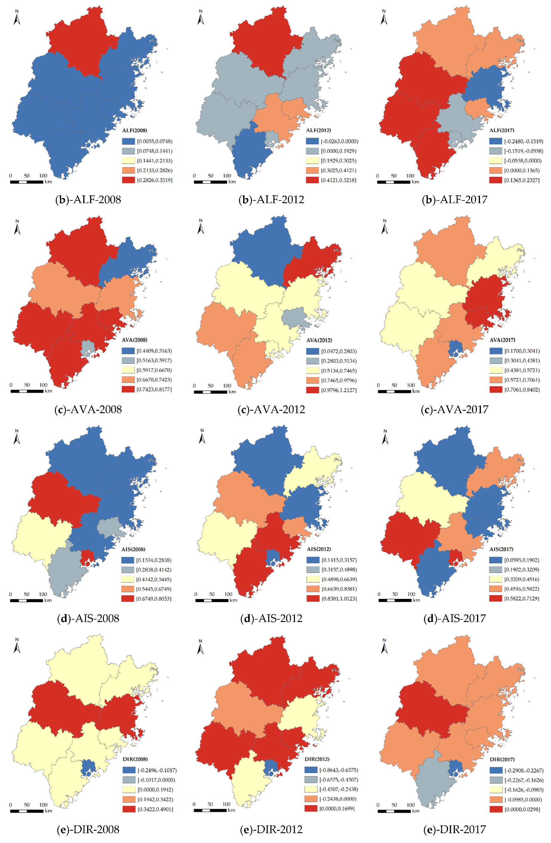
4.3.2. The Influence of ALF on Agricultural Carbon Emissions

The results listed in Table 5 show that ALF significantly promoted the increase of agricultural carbon emissions. That is, when ALF increased by 1%, agricultural carbon emissions increased by an average of 0.0512%. One possible explanation is that the disorderly increase of ALF enlarged the scale of agricultural production to a certain extent, which was not conducive to reducing the agricultural carbon emissions. As shown in Figure 2b, the increase of ALF in all prefectural-level cities promoted the increase of agricultural carbon emissions, and the positive influence of ALF on agricultural carbon emissions in Nanping was the strongest. Nanping’s agricultural labor force accounted for nearly 50% of the total labor force, which had a strong role in promoting agricultural carbon emissions. Moreover, the ALF in Quanzhou in 2012 and in Fuzhou, Quanzhou, and Xiamen in 2017 demonstrated negative correlations with agricultural carbon emissions, which was inconsistent with the significant positive correlation results of other relevant literature. The possible reason is that ALF showed obvious spatial heterogeneity. That is, Fuzhou, Quanzhou, and Xiamen have been facing a rapid development of economic and agricultural modernization in recent years. With the vigorous support of human resources and financial policies, the increase of ALF has brought advanced technology and professionals, improved the level of agricultural technology, and thus, to a certain extent, restrained the large growth of carbon emissions. However, the relationship between ALF and agricultural carbon emissions in other cities is significantly positive, which makes it more important to think about how to train the labor force in other regions and formulate corresponding policies to attract talents in the progress of agricultural technological innovation, so as to restrain agricultural carbon emissions.

The increase of the agricultural labor force in Fujian has promoted agricultural carbon emissions as a whole. However, in Fuzhou, Quanzhou, and Xiamen, the increase of technical personnel and the improvement of the quality of the agricultural labor force can reduce agricultural carbon emissions. Therefore, on the one hand, the government needs to guide actively the transfer of rural surplus labor to manufacturing and service industries, so as to reduce the agricultural labor force. On the other hand, the government needs to improve the education level of rural residents and strengthen their low carbon awareness, so that farmers can rationally use advanced agricultural technology. At the same time, the government needs to establish, improve, and strengthen the training and introduction of high-quality agricultural technological talents and provide human support for agricultural modernization.

4.3.3. The Influence of AVA on Agricultural Carbon Emissions

AVA significantly promoted the increase of agricultural carbon emissions and mainly promoted the average increases of agricultural carbon emissions by 0.6955% when AVA increased by 1%. That is, AVA is the main driving factor for the increase of agricultural carbon emissions. Besides, Fujian is a populous province, but the land resources are limited, so agriculture depends on chemical fertilizer and pesticides to meet people’s demand for agricultural products and agricultural by-products, which also leads to the increase of AVA and the sharp increase of agricultural carbon emissions. As shown in Figure 2c, in 2008, 2012, and 2017, the regression coefficients of AVA in all prefectural-level cities in Fujian were all positive, and there was no obvious downward trend. Besides, AVA in Putian, Quanzhou, and Zhangzhou had a stronger impact on agricultural carbon emissions. For instance, in 2017, AVA in Putian, Quanzhou, and Zhangzhou accounted for nearly 2.9322%, 9.9831%, and 19.9504% of Fujian’s total AVA, respectively, while chemical fertilizer use accounted for 5.0622%, 12.4713%, and 32.2809% of Fujian’s total chemical fertilizer use, respectively. However, it should be noted that there existed a tendency of diminishing marginal utility in the use of chemical fertilizers, pesticides, plastic sheeting, and other products. It is obviously unsustainable for AVA to depend too much on the inputs of pesticides and fertilizers, nor can it enhance the comprehensive production capacity of agriculture.

Although AVA promotes agricultural carbon emissions, it cannot reduce agricultural carbon emissions by directly reducing the added value of agriculture. Thus, the increase of AVA mainly depends on the progress of agricultural technology and the promotion of production efficiency, so as to achieve the dual objectives of increasing AVA and controlling agricultural carbon emissions, and this can also fundamentally reduce the positive impact of AVA on agricultural carbon emissions.

4.3.4. The Influence of AIS on Agricultural Carbon Emissions

According to Table 5, AIS significantly promoted the increase of agricultural carbon emissions. That is, when AIS increased by 1%, agricultural carbon emissions increased by 0.4426% on average in the same direction. This shows that the plant products industry is the main source of agricultural carbon emissions, and the increase of its proportion will correspondingly increase the total carbon emissions. According to Figure 2d, AIS in Fuzhou had less influence on agricultural carbon emissions. This is mainly due to the high proportion of the fishery industry in Fuzhou’s agricultural structure. In 2017, the proportion of the fishery industry output in Fuzhou’s agricultural sector output reached 58%. Moreover, although the proportion of the plant products industry in Zhangzhou is inferior to Sanming, nearly 50%, the influence of AIS on agricultural carbon emissions was less. The results in Figure 2d also show that the coefficient of AIS in Zhangzhou was 0.3665 in 2008, 0.2055 in 2012, and 0.0903 in 2017, which shows a large downward trend. The possible reason is that the cultivated land in Zhangzhou is relatively concentrated and flat, which is suitable for large-scale mechanized farming. That is, the mechanized level of the plant products industry in Zhangzhou has reached the leading level. Thus, the development of the plant products industry would promote the increase of agricultural carbon emissions, but the influence was less, which is closely related to the production mode of its own planting industry.

AIS was second only to AVA in promoting agricultural carbon emissions. Thus, on the premise of food security, the government should actively optimize the structure of agriculture, guide farmers to reduce the planting of crops with high resource input and energy consumption, then increase the proportion of low-carbon productions such as fruits, flowers, and vegetables. This can not only improve the economic benefits, but also have a certain carbon-sink function. Besides, AIS played the most important role in promoting agricultural carbon emissions in Xiamen and Sanming. Thus, Xiamen and Sanming should further reduce the proportion of the planting industry. For instance, Xiamen can take advantage of its coastal location to develop fisheries and flowers, while Sanming can continue to develop special forestry industries such as Camellia oleifera, bamboo shoots, and forest tourism.

4.3.5. The Influence of DIR on Agricultural Carbon Emissions

DIR significantly inhibited the increase of agricultural carbon emissions. When DIR increased by 1%, agricultural carbon emissions decreased by 0.0711% on average. As a whole, the relationship between per capita disposable income of rural residents and environmental pollution in Fujian has jumped over the turning point of the inverted “U” shape and reached the right side. It has entered the stage that the more the agricultural economy develops, the smaller the agricultural carbon emissions. Under these circumstances, on the one hand, the increase of disposable income of rural residents can promote farmers to adopt modern machinery in agricultural production, improve the mechanization level and agricultural production efficiency, and then achieve the effect of increasing production and reducing carbon emissions. On the other hand, the increase of rural residents’ disposable income can encourage farmers to choose less polluting products, such as organic fertilizer and bio-fertilizer, so as to reduce agricultural carbon emissions. As shown in Figure 2e, in 2008, only Xiamen’s DIR was negatively correlated with agricultural carbon emissions. In 2012, the relationship between DIR and environmental pollution in Fuzhou, Quanzhou, and Zhangzhou also surpassed the turning point of the inverted “U” shape, and DIR was negatively correlated with agricultural carbon emissions. In 2017, except Sanming, the increase of DIR in the other eight prefectural-level cities all reduced agricultural carbon emissions, indicating that DIR of Sanming had not reached the inflection point of the environmental Kuznets curve, and the increase of DIR at this stage increased agricultural carbon emissions.

The increase of DIR can significantly inhibit agricultural carbon emissions. The governments can adopt diversified policies to increase rural residents’ disposable income. For areas with rural economic underdevelopment, such as Longyan, Ningde, Sanming, and Nanping, the governments can reduce the cost of agricultural production through fiscal policies and the promotion of agricultural mechanization. The governments can also help these areas establish and develop leading industries through planning guidance and technical services. For cities with large plains, i.e., Putian, Quanzhou, Zhangzhou, and Fuzhou, the governments can guide the transfer of agricultural labor forces to non-agricultural industries, make the agricultural labor force employ more agricultural production materials, and expand the scale of agricultural operation, increasing the income of agricultural workers. In addition, Xiamen has a relatively high degree of industrialization and urbanization. The government can vigorously develop the processing industry of agricultural products and promote the integration of the industries. In addition, in 2017, except Sanming, the relationship between DIR and agricultural carbon emissions has jumped the turning point of the inverted “U” shape. Therefore, Sanming should transfer its environmental Kuznets curve to the decline stage of the inverted “U” shape, that is to take into account the dual responsibilities of income growth and agricultural carbon emission reduction.

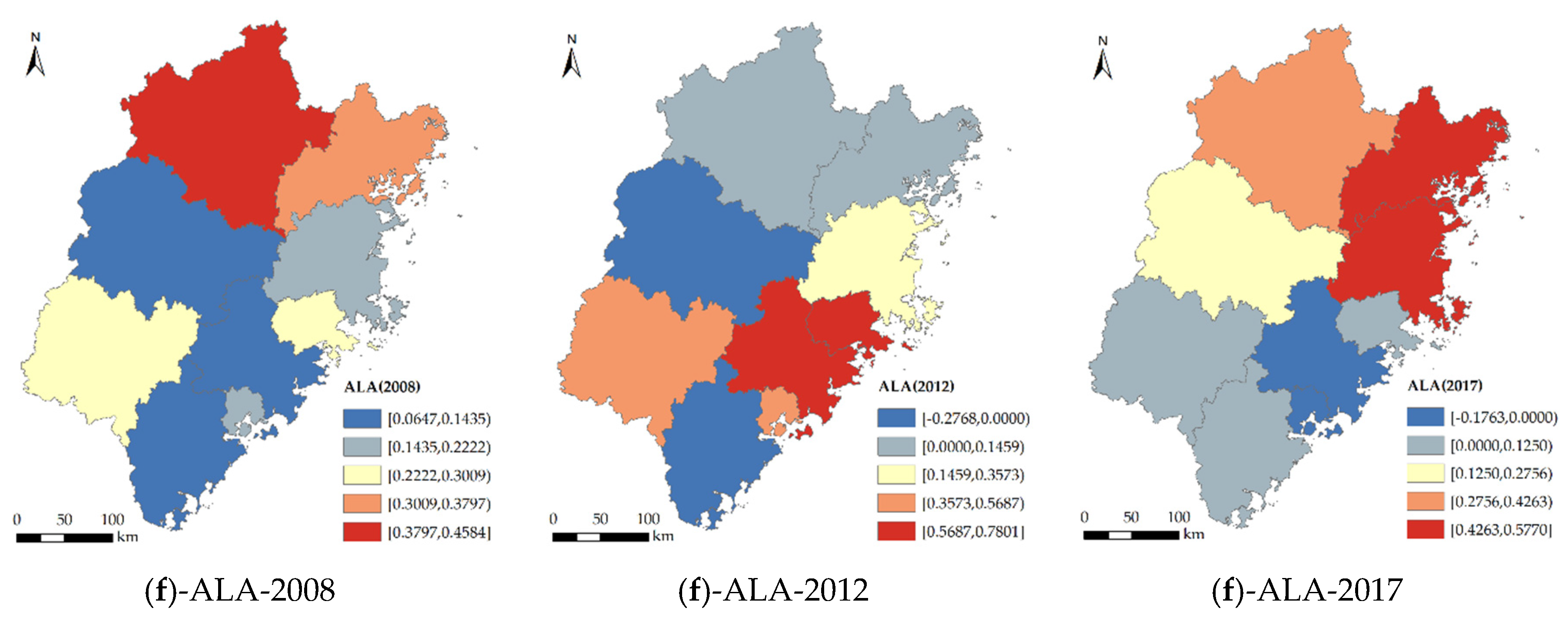
4.3.6. The Influence of ALA on Agricultural Carbon Emissions

According to Table 5, ALA significantly promoted the increase of agricultural carbon emissions. ALA mainly promoted the average increases of agricultural carbon emissions by 0.2873% when ALA increased by 1%. As shown in Figure 2f, the positive impact of ALA on agricultural carbon emissions mainly existed in the northern cities, especially in Ningde and Nanping. In comparison, Xiamen and Quanzhou, which are located in the southern part, became the cities where arable land area had a negative influence on agricultural carbon emissions in 2017. A possible explanation for this is due to the high level of industrialization and urbanization in Quanzhou and Xiamen. In these two cities, agricultural land has been gradually transformed into industrial land, and the arable land area has been seriously insufficient. However, economic development and residents’ demand for agricultural products have led to the high investment and intensive use of arable land, which leads to the increase of agricultural carbon emissions beyond the land carrying threshold. Besides, the ALA of Putian and Longyan had little impact on agricultural carbon emissions, which is related to the policy of “returning farmland to forestry” in the two cities. Farmland with serious pollution and declining soil biological activity stopped being tilled and gradually turned into woodland. Meanwhile, reclamation of exploitable barren hills could reduce the promotion of arable land area on agricultural carbon emissions.

There exists a positive correlation between ALA and agricultural carbon emissions, but if the government blindly returns farmland to forestry or converts agricultural land into industrial land, it may also increase agricultural carbon emissions. Thus, the governments should develop and utilize the land rationally and optimize the land use structure. For instance, the governments of Quanzhou and Xiamen should control the total amount of industrial land to avoid the serious shortage of arable land threatening food security and bringing about the large use of energy products. Similarly, Ningde and Fuzhou can implement cultivated land protection measures to improve the ecological carrying capacity of agricultural land, that is to stop cultivating land with serious pollution and the decline of soil biological activity, and gradually turn it into woodland or grassland.

5. Conclusions

This paper measured agricultural carbon emissions in Fujian Province based on carbon emission coefficients released by IPCC and WRI, then applied GTWR to test empirically the influencing factors on agricultural carbon emissions. As a whole, the main conclusions can be listed as follows:

(1) Average agricultural carbon emissions in Fujian decreased from 708.88 × 10³ tonnes of carbon in 2008 to 615.78 × 10³ tonnes of carbon in 2017, and total agricultural carbon emissions showed a fluctuating downward trend. The fluctuating evolution with the basic spatial pattern of “M” can be divided into four stages: fluctuating increase, low speed reduction, rapid increase, and finally, rapid reduction. In addition, among all kinds of carbon sources, agricultural land use had the largest agricultural carbon emissions, followed by rice paddies and livestock manure storage, accounting for 40.92%, 34.48%, and 13.26% of the total agricultural carbon emissions in Fujian in 2017, respectively.

(2) From the perspective of direction, among factors affecting agricultural carbon emissions in Fujian, RDI and DIR mainly had inhibitory effects, while ALF, AVA, AIS, and ALA had promoting effects. From the perspective of degree, AVA had the greatest influence, followed by AIS and ALA. When these three factors changed by 1%, agricultural carbon emissions would change by 0.6955%, 0.4426%, and 0.2873% on average, respectively.

(3) According to the GTWR regression results, the six factors selected in this paper had different directions and different degrees of effects on the nine prefectural-level cities in Fujian Province. For instance, ALF mainly inhibited agricultural carbon emissions in Fuzhou and Xiamen, but promoted agricultural carbon emissions in other cities. Moreover, the effect of RDI and DIR on agricultural carbon emissions in eastern Fujian was stronger than that in western Fujian. Besides, for Xiamen, the main factor affecting agricultural carbon emissions was AIS, but for other cities of Fujian, the main factor was AVA. Therefore, it is necessary to adopt different means to reduce carbon emissions according to the actual situation.

(4) Combining the total amount of agricultural carbon emissions and the spatial and temporal characteristics of the influencing factors in Fujian, some policy recommendations can be put forward to achieve the ultimate goal of reducing agricultural carbon emissions.

References

1. Lamb, A.; Green, R.; Bateman, I.; Broadmeadow, M.; Bruce, T.; Burney, J.; Carey, P.; Chadwick, D.; Crane, E.; Field, R.; et al. The potential for land sparing to offset greenhouse gas emissions from agriculture. Nat. Clim. Chang. 2016, 6, 488–492. [Google Scholar] [CrossRef] [Green Version]
2. Pellerin, S.; Bamiere, L.; Angers, D.; Beline, F.; Benoit, M.; Butault, J.P.; Chenu, C.; Colnenne-David, C.; De Cara, S.; Delame, N.; et al. Identifying cost-competitive greenhouse gas mitigation potential of French agriculture. Environ. Sci. Policy 2017, 77, 130–139. [Google Scholar] [CrossRef] [Green Version]
3. Nayak, D.; Saetnan, E.; Cheng, K.; Wang, W.; Koslowski, F.; Cheng, Y.F.; Zhu, W.Y.; Wang, J.K.; Liu, J.X.; Moran, D.; et al. Management opportunities to mitigate greenhouse gas emissions from Chinese agriculture. Agric. Ecosyst. Environ. 2015, 209, 108–124. [Google Scholar] [CrossRef] [Green Version]
4. Wang, W.; Koslowski, F.; Nayak, D.R.; Smith, P.; Saetnan, E.; Ju, X.T.; Guo, L.D.; Han, G.; de Perthuis, C.; Lin, E.; et al. Greenhouse gas mitigation in Chinese agriculture: Distinguishing technical and economic potentials. Glob. Environ. Chang. 2014, 26, 53–62. [Google Scholar] [CrossRef] [Green Version]
5. ACIL Tasman Pty Ltd. Agriculture and GHG Mitigation Policy: Options in Addition to the CPRS; Industry & Investment NSW: Dubbo, Australia, 2009; Available online: http://farminstitute.org.au/LiteratureRetrieve.aspx?ID=53067 (accessed on 13 August 2019).
6. Eggleston, S.; Buendia, L.; Miwa, K.; Ngara, T.; Tanabe, K. Volume 4: Agriculture, forestry and other land use. In 2006 IPCC Guidelines for National Greenhouse Gas Inventories; Cambridge University Press: Cambridge, UK, 2006. [Google Scholar]
7. Wang, W.; Guo, L.P.; Li, Y.C.; Su, M.; Lin, Y.B.; de Perthuis, C.; Ju, X.T.; Lin, E.D.; Moran, D. Greenhouse gas intensity of three main crops and implications for low-carbon agriculture in China. Clim. Chang. 2015, 128, 57–70. [Google Scholar] [CrossRef]
8. Xiong, C.H.; Yang, D.G.; Xia, F.Q.; Huo, J.W. Changes in agricultural carbon emissions and factors that influence agricultural carbon emissions based on different stages in Xinjiang, China. Sci. Rep. 2016, 6, 36912. [Google Scholar] [CrossRef] [PubMed] [Green Version]
9. Tian, J.X.; Yang, H.L.; Xiang, P.A.; Liu, D.W.; Li, L. Drivers of agricultural carbon emissions in Hunan Province, China. Environ. Earth Sci. 2016, 75, 121. [Google Scholar] [CrossRef]
10. Han, H.B.; Zhong, Z.Q.; Guo, Y.; Xi, F.; Liu, S.L. Coupling and decoupling effects of agricultural carbon emissions in China and their driving factors. Environ. Sci. Pollut. Res. 2018, 25, 25280–25293. [Google Scholar] [CrossRef]
11. Zhang, L.; Pang, J.X.; Chen, X.P.; Lu, Z. Carbon emissions, energy consumption and economic growth: Evidence from the agricultural sector of China’s main grain-producing areas. Sci. Total Environ. 2019, 665, 1017–1025. [Google Scholar] [CrossRef]
12. Bell, M.J.; Cloy, J.M.; Rees, R.M. The true extent of agriculture’s contribution to national greenhouse gas emissions. Environ. Sci. Policy 2014, 39, 1–12. [Google Scholar] [CrossRef]
13. Wisniewski, P.; Kistowski, M. Assessment of greenhouse gas emissions from agricultural sources in order to plan for needs of low carbon economy at local level in Poland. Geogr. Tidsskr.-Den. 2018, 118, 123–136. [Google Scholar] [CrossRef]
14. Yue, Q.; Xu, X.R.; Hillier, J.; Cheng, K.; Pan, G.X. Mitigating greenhouse gas emissions in agriculture: From farm production to food consumption. J. Clean. Prod. 2017, 149, 1011–1019. [Google Scholar] [CrossRef]
15. Ismael, M.; Srouji, F.; Boutabba, M.A. Agricultural technologies and carbon emissions: Evidence from Jordanian economy. Environ. Sci. Pollut. Res. 2018, 25, 10867–10877. [Google Scholar] [CrossRef]
16. Gomiero, T.; Paoletti, M.G.; Pimentel, D. Energy and environmental issues in organic and conventional agriculture. Crit. Rev. Plant Sci. 2008, 27, 239–254. [Google Scholar] [CrossRef]
17. Cui, H.R.; Zhao, T.; Shi, H.J. STIRPAT-based driving factor decomposition analysis of agricultural carbon emissions in Hebei, China. Pol. J. Environ. Stud. 2018, 27, 1449–1461. [Google Scholar] [CrossRef]
18. Gerlagh, R. Measuring the value of induced technological change. Energy Policy 2007, 35, 5287–5297. [Google Scholar] [CrossRef]
19. Zhao, R.Q.; Liu, Y.; Tian, M.M.; Ding, M.L.; Cao, L.H.; Zhang, Z.P.; Chuai, X.W.; Xiao, L.G.; Yao, L.G. Impacts of water and land resources exploitation on agricultural carbon emissions: The water-land-energy-carbon nexus. Land Use Policy 2018, 72, 480–492. [Google Scholar] [CrossRef]
20. Lu, X.H.; Kuang, B.; Li, J.; Han, J.; Zhang, Z. Dynamic evolution of regional discrepancies in carbon emissions from agricultural land utilization: Evidence from Chinese provincial data. Sustainability 2018, 10, 552. [Google Scholar] [CrossRef]
21. Sarauer, J.L.; Coleman, M.D. Converting conventional agriculture to poplar bioenergy crops: Soil greenhouse gas flux. Scand. J. For. Res. 2018, 33, 781–792. [Google Scholar] [CrossRef]
22. West, T.O.; Marland, G. Net carbon flux from agriculture: Carbon emissions, carbon sequestration, crop yield, and land-use change. Biogeochemistry 2003, 63, 73–83. [Google Scholar] [CrossRef]
23. Zafeiriou, E.; Mallidis, I.; Galanopoulos, K.; Arabatzis, G. Greenhouse gas emissions and economic performance in EU agriculture: An empirical study in a non-linear framework. Sustainability 2018, 10, 3837. [Google Scholar] [CrossRef]
24. Owusu, P.A.; Asumadu-Sarkodie, S. Is there a causal effect between agricultural production and carbon dioxide emissions in Ghana? Environ. Eng. Res. 2017, 22, 40–54. [Google Scholar] [CrossRef]
25. Khan, M.; Ali, Q.; Ashfaq, M. The nexus between greenhouse gas emission, electricity production, renewable energy and agriculture in Pakistan. Renew. Energy 2018, 118, 437–451. [Google Scholar] [CrossRef]
26. Liu, X.; Zhang, S.; Bae, J. The impact of renewable energy and agriculture on carbon dioxide emissions: Investigating the environmental Kuznets curve in four selected ASEAN countries. J. Clean. Prod. 2017, 164, 1239–1247. [Google Scholar] [CrossRef]
27. Mourao, P.R.; Martinho, V.D. Portuguese agriculture and the evolution of greenhouse gas emissions-can vegetables control livestock emissions? Environ. Sci. Pollut. Res. 2017, 24, 16107–16119. [Google Scholar] [CrossRef]
28. Xiong, C.H.; Yang, D.G.; Huo, J.W. Spatial-temporal characteristics and LMDI-based impact factor decomposition of agricultural carbon emissions in Hotan Prefecture, China. Sustainability 2016, 8, 262. [Google Scholar] [CrossRef]
29. Tian, Y.; Zhang, J.B.; He, Y.Y. Research on spatial-temporal characteristics and driving factor of agricultural carbon emissions in China. J. Integr. Agric. 2014, 13, 1393–1403. [Google Scholar] [CrossRef]
30. Appiah, K.; Du, J.G.; Poku, J. Causal relationship between agricultural production and carbon dioxide emissions in selected emerging economies. Environ. Sci. Pollut. Res. 2018, 25, 24764–24777. [Google Scholar] [CrossRef]
31. Yadav, D.; Wang, J.Y. Modelling carbon dioxide emissions from agricultural soils in Canada. Environ. Pollut. 2017, 230, 1040–1049. [Google Scholar] [CrossRef]
32. Ye, R.; Espe, M.B.; Linquist, B.; Parikh, S.J.; Doane, T.A.; Horwath, W.R. A soil carbon proxy to predict CH4 and N2O emissions from rewetted agricultural peatlands. Agr. Ecosyst. Environ. 2016, 220, 64–75. [Google Scholar] [CrossRef] [Green Version]
33. Jiang, X.; Fang, W.; Zhuang, G.; Bai, W.; Zhu, S.; Lu, L.; Feng, J. Greenhouse Gas Accounting Tool for Chinese Cities (Version 2.0); World Resources Institute: Washington, DC, USA, 2015. [Google Scholar]
34. Snyder, C.S.; Davison, E.A.; Smith, P.; Venterea, R.T. Agriculture: Sustainable crop and animal production to help mitigate nitrous oxide emissions. Curr. Opin. Environ. Sustain. 2014, 9, 46–54. [Google Scholar] [CrossRef]
35. Sasmal, T.K. Adoption of new agricultural technologies for sustainable agriculture in eastern India: An empirical study. Indian Res. J. Ext. Educ. 2015, 15, 38–42. [Google Scholar]
36. Xiong, C.H.; Yang, D.G.; Huo, J.W.; Zhao, Y.N. The relationship between agricultural carbon emissions and agricultural economic growth and policy recommendations of a low-carbon agriculture economy. Pol. J. Environ. Stud. 2016, 25, 2187–2195. [Google Scholar] [CrossRef]
37. You, D.; Jiang, K. Research into dynamic lag effect of R&D input on economic growth based on the vector auto-regression model. J. Comput. Theor. Nanosci. 2016, 13, 6787–6796. [Google Scholar]
38. Zhang, Y.; Fang, G. Research on spatial-temporal characteristics and affecting factors decomposition of agricultural carbon emission in Suzhou City, Anhui Province, China. Appl. Mech. Mater. 2013, 291, 1385–1388. [Google Scholar] [CrossRef]
39. Yao, C.; Qian, S.; Mao, Y.; Li, Z. Decomposition of impacting factors of animal husbandry carbon emissions change and its spatial differences in China. Trans. Chin. Soc. Agric. Eng. 2017, 33, 10–19. (In Chinese) [Google Scholar]
40. Satterthwaite, D. The implications of population growth and urbanization for climate change. Environ. Urban. 2009, 21, 545–567. [Google Scholar] [CrossRef] [Green Version]
41. Al-Mulali, U.; Sab, C.N.B.S.; Fereidouni, H.G. Exploring the bi-directional long run relationship between urbanization, energy consumption, and carbon dioxide emission. Energy 2012, 46, 156–167. [Google Scholar] [CrossRef]
42. Murad, W.; Ratnatunga, J. Carbonomics of the Bangladesh agricultural output: Causality and long-run equilibrium. Manag. Environ. Qual. An Int. J. 2013, 24, 256–271. [Google Scholar] [CrossRef]
43. Jebli, M.B.; Youssef, S.B. The role of renewable energy and agriculture in reducing CO2, emissions: Evidence for North Africa countries. Ecol. Indic. 2015, 74, 295–301. [Google Scholar] [CrossRef]
44. Rafiq, S.; Salim, R.; Apergis, N. Agriculture, trade openness and emissions: An empirical analysis and policy options. Aust. J. Agric. Resour. Econ. 2016, 60, 348–365. [Google Scholar] [CrossRef]
45. Alamdarlo, N.H. Water consumption, agriculture value added and carbon dioxide emission in Iran, environmental Kuznets curve hypothesis. Int. J. Environ. Sci. Technol. 2016, 13, 2079–2090. [Google Scholar] [CrossRef]
46. Panayotou, T. Empirical Tests and Policy Analysis of Environmental Degradation at Different Stages of Economic Development; World Employment Research Programme, Working Paper; International Labour Office: Geneva, Switzerland, 1993. [Google Scholar]
47. Liu, L.H.; Xin, H.P. Research on spatial-temporal characteristics of agricultural carbon emissions in Guangdong Province and the relationship with economic growth. Adv. Mater. Res. 2014, 1010, 2072–2079. [Google Scholar] [CrossRef]
48. Zhang, J.; Yuan, C.; Zhang, L.; Ding, L. Do technological innovations promote urban green development?—A spatial econometric analysis of 105 cities in China. J. Clean. Prod. 2018, 182, 395–403. [Google Scholar] [CrossRef]
49. Li, X.; Jiang, D.; Bian, Z.; Yan, J.; Qu, F. China cultivated land change and its carbon budget measurement based on the system dynamics. World Agric. 2015, 7, 19–24. [Google Scholar]
50. Smith, P.; Martino, D.; Cai, Z.; Gwary, D.; Janzen, H.; Kumar, P.; McCarl, B.; Ogle, S.; O’Mara, F.; Rice, C.; et al. Greenhouse gas mitigation in agriculture. Philos. Trans. R. Soc. B Biol. Sci. 2008, 363, 789–813. [Google Scholar] [CrossRef]
51. Yager, R.R. On ordered weighted averaging aggregation operators in multicriteria decisionmaking. Read. Fuzzy Sets Intell. Syst. 1988, 18, 80–87. [Google Scholar] [CrossRef]
52. Xu, Z. An overview of methods for determining OWA weights. Int. J. Intell. Syst. 2005, 20, 843–865. [Google Scholar] [CrossRef]
53. Brunsdon, C.; Fotheringham, A.S.; Charlton, M.E. Geographically weighted regression: A method for exploring spatial nonstationarity. Geogr. Anal. 1996, 28, 281–298. [Google Scholar] [CrossRef]
54. Brunsdon, C.; Fotheringham, A.S.; Charlton, M. Some notes on parametric significance tests for geographically weighted regression. J. Reg. Sci. 1999, 39, 497–524. [Google Scholar] [CrossRef]
55. Li, M.; Wang, J.; Chen, Y. Evaluation and influencing factors of sustainable development capability of agriculture in countries along the Belt and Road route. Sustainability 2019, 11, 2004. [Google Scholar] [CrossRef]
56. Huang, B.; Wu, B.; Barry, M. Geographically and temporally weighted regression for modeling spatio-temporal variation in house prices. Int. J. Geogr. Inf. Sci. 2010, 24, 383–401. [Google Scholar] [CrossRef]
57. He, Q.; Bo, H. Satellite-based high-resolution PM 2.5 estimation over the Beijing-Tianjin-Hebei region of China using an improved geographically and temporally weighted regression model. Environ. Pollut. 2018, 236, 1027–1037. [Google Scholar] [CrossRef]
58. Mohamad, R.S.; Verrastro, V.; Al Bitar, L.; Roma, R.; Moretti, M.; Al Chami, Z. Effect of different agricultural practices on carbon emission and carbon stock in organic and conventional olive systems. Soil Res. 2016, 54, 173–181. [Google Scholar] [CrossRef]
Figure 1. The location of the study area.
Energies 12 03102 g001
Figure 2. Spatial distribution of regression coefficients calculated by GTWR in 2008, 2012, and 2017.
Energies 12 03102 g002aEnergies 12 03102 g002bEnergies 12 03102 g002c